Incorporating Stakeholders’ priorities and preferences in 4D trajectory optimization

Incorporating Stakeholders’ Priorities and Preferences in

4D Trajectory Optimization

Veronica Dal Sasso

Franklin Djeumou Fomeni

Guglielmo Lulli

Konstantinos Zografos

Abstract

A key feature of trajectory based operations (TBO) – a new concept developed to modernize the air traffic system – is the inclusion of preferences and priorities of the air traffic management (ATM) stakeholders. In this paper, we present a new math-ematical model to optimize flights’ 4D-trajectories. This is a multi-objective binary integer programming (IP) model, which assigns a 4D-trajectory to each flight, while explicitly modeling priorities and highlighting the trade off involved with the Airspace Users (AUs) preferences. The scope of the model (to be used at pre-tactical level) is the computation of optimal 4D pre-departure trajectory for each flight to be shared or negotiated with other stakeholders and subsequently managed throughout the flight. These trajectories are obtained by minimising the deviation (delay and re-routing) from the original preferred 4D-trajectories as well as minimizing the air navigation service (ANS) charges subject to the constraints of the system. Computational results for the model are presented, which show that the proposed model has the ability to identify trade-offs between the objectives of the stakeholders of the ATM system under the TBO concept. This can therefore provide the ATM stakeholders with useful decision tools to choose a trajectory for each flight.

Keywords: integer programming (IP); Air Traffic Flow Management (ATFM); Tra-jectory Based Operations (TBO); multi-objective optimization; 4D-Trajectories; Stake-holders’ priorities and preferences.

1

Introduction

The challenge growth report [2] of the European Organization for the Safety of Air Naviga-tion (EUROCONTROL) forecasts that the air traffic system in Europe is to record about 14.4 million flights in 2035, which will represent 1.5 times the level of traffic recorded in 2012. Furthermore, the corresponding number of passengers is expected to double from 0.7 billion in 2012 to 1.4 billion passengers in 2035. Such a dramatic growth brings up many challenges that need to be tackled to ensure the sustainability and competitiveness of avi-ation in Europe. For example, it is forecasted in [2] that about 1.9 million flights may not be accommodated in 2035 with the current concept of operations. This is the equivalent of

∗_{Department of Management Science, Lancaster University, Lancaster LA1 4YX, United}

Kingdom. Emails: [email protected], [email protected], [email protected], [email protected].

120 million passengers that may not be able to travel. Among many other challenges that will come along with such a growth are the environmental impact, the cost and operational efficiency of the system (e.g. reducing flight time, fuel burn, route charges per flight), as well as safety and security.

As a response to such a dramatic growth, the European Commission has adopted the Single European Sky framework as a legislative framework for European aviation. While the Air Traffic Management (ATM) system migrates towards this concept vision, some sig-nificant changes have been identified as described in the Global ATM Operational Concept [31]. One such change, Trajectory Based Operations (TBO) , is described as follows [31]: “Air traffic management (ATM) considers the trajectory of a manned or unmanned vehicle during all phases of flight and manages the interaction of that trajectory with other tra-jectories or hazards to achieve the optimum system outcome, with minimal deviation from the user-requested flight trajectory, whenever possible.” TBO represents a shift from present operations towards the use of a shared trajectory, collaboratively developed as the basis for decision-making across the ATM System Participants. It is identified in both the European ATM Master Plan [1] and the Single European Sky ATM Research (SESAR) Concept of Operations [3] as one of the cornerstones of the future ATM system. It also provides an op-portunity to shift operations towards greater predictability with flight-impacting decisions being coordinated across concept components. The main differences with today’s operation involve:

1. Sharing of trajectory information eventually leading to a common view of the trajec-tory.

2. Managing trajectory information using Collaborative Decision Making (CDM).

3. The trajectory that is shared and managed, the Agreed Trajectory, is used as reference for the flight by providing a common intent to be achieved during the execution of the flight.

The TBO concept is expected to benefit the ATM system in many aspects. For example, the ATM community will contribute to the protection of the environment by taking into con-sideration the consequences of airspace activities. Moreover, the management of trajectory and the exchange of information between airspace users (AUs) and the ATM system will improve conflict management and facilitate the use of preferred trajectories for each flight. More detailed descriptions of the TBO concept and its benefits can also be found in [32]. The development and implementation of the TBO concept require the development of opti-mization models and algorithms that will allow pertinent decision makers and stakeholders to examine the trade-offs between user and system optimum trajectories and to facilitate the definition of commonly accepted trajectories by all stakeholders.

negotiation and acceptability of trajectories between the stakeholders. Indeed, the model considers the preferred 4D-trajectory of all the flights in the pre-tactical planning phase and outputs the set of all the non-dominated optimal solutions that can be implemented by the network manager. Each of these non-dominated solutions consists of pre-departure 4D-trajectories to be shared or negotiated with other stakeholders and subsequently managed throughout the flight. We consider the following three objectives for optimization:

i) Minimization of the total time deviation (delay) from the scheduled time of operations. The delay function is a combination of airborne delay and ground holding delay, which is less costly than airborne delay.

ii) Minimization of the cost of deviation from the users preferred 3D-routes (lateral and vertical deviation). This represents the cost of fuel burnt when a flight uses a particular 3D-route.

iii) Minimization of the airspace navigation service (ANS) charges. These costs are in-curred when flights travel through the charging zones defined by the states in the ECAC area.

The above objective functions represent some of the key performance indicators (KPIs) of improvement targeted by the TBO concept [3]. They were identified as results of a consultation activity with the European ATM stakeholders, who also expressed their views on how their priorities and preferences could be incorporated in our model [28].

Since our proposed model is formulated as a tri-objective integer program, we imple-ment the quadrant shrinking method (QSM) of Boland et al [34] in order to compute the pareto frontier. The iterations of this method require solving two single-objective integer programs, each of which is solved using the branch-and-cut algorithm. An extensive set of computational experiments has been carried out with large scale instances and the results of these experiments are presented in this paper along with some insightful analyses of the trade-offs between the above mentioned conflicting objective functions.

In the subsequent sections of the paper, we will i) highlight the expectation of the ATM stakeholders with respect to the TBO concept in Section 2; ii) provide a brief review of the literature relevant to our research in Section3; iii) present our mathematical model in Section4; iv) present the solution approach for solving the model in Section5; v) discuss the computational experiments conducted in Section6; vi) end with some concluding remarks in Section7.

2

Stakeholders expectations and inputs

With the deployment of the TBO concept, AUs expect to be given more flexibility in order to better manage their own flights and meet their internal business models. Indeed, the network manager sees every flight as equal, while for the airlines each flight is unique. Since even a small change to some flights may have a bigger economic impact for airlines. Therefore, AUs expect their preferences and priorities to be taken into consideration in the decision making process.

2.1

Modelling methodology

Figure 1. Modelling methodology(from [15,16])

framework as presented in Figure 1 (from [15, 16]) . We organized a workshop with the European ATM stakeholders. The objectives of this workshop were to elicit the views about the preferences and priorities of the ATM stakeholders in relation to the optimization of flights trajectories, and also to identify the key performance areas (KPAs) and key perfor-mance indicators (KPIs) for assessing how our model could meet their expectations with respect to the TBO concept. The outcome of this consultation enabled us to develop the mathematical model presented in this paper. It also set the guideline of how the preferences and the priorities of the AUs can be integrated in our optimization model. Interested readers are referred to [28] for the report of this consultation activity.

2.2

Preferences

stakeholders are also captured in terms of how well each of the objective functions achieves their individual interests.

2.3

Priorities

The prioritization scheme can be regarded as a framework which will provide the airspace users with the flexibility of managing and adapting their internal business model in a con-strained environment [20]. To this end, SESAR has developed the concept of User-Driven Prioritization Process (UDPP) [22], which enables the airspace users to optimize their flight schedules by managing time deviation (delays) during departure, en-route and arrival. In other words, UDPP provides the airspace users with the capability of prioritizing their flights in case of capacity-constrained planning. The first step of UDPP is limited to departure slot swapping at tactical level [21]. UDPP Step 2 is foreseen beyond slot swapping and is considered at the planning phase. Our model considers prioritization at the planning phase. A SESAR research activity [22] proposes a prioritization mechanism (called the Fleet Delay Apportionment or FDA) wherein airspaces users assign priority values to their flights and the system apportions delays to flights proportionally to their priority values. The allowable priority values are integers 1 through 9, with a value of 1 indicating the highest priority and of 9 indicating the lowest priority. We denote these priority values byτf for each flightf.

The overall idea of prioritization is for the AUs to decide how the total delay of their own fleet should be apportioned among their flights. Therefore, our mathematical model will capture the priorities through constraints which set the maximum amount of delay to be absorbed by each flight. More precisely, if we let σf be the baseline delay (i.e. delay

when prioritization is not allowed) of flightf and Φ the set of all the airspace users, with an AU beingφ∈Φ, then the maximum amount of delayγf to be assigned to flightf under

the FDA mechanism is calculated as [20]:

γf =



 

τf.σf

P

f∈Fφ

τf.σf





.ζφ, (1)

whereζφ= P f∈Fφ

σfwithφ∈Φ is the total amount of delay to be absorbed by airspace userφ

in the baseline delay, withFφ being the fleet of AUφ. In more detail, the FDA mechanism

works as follows. First the AUs submits their preferred flight trajectories request to the system. The network manager runs simulation with these flight plans to determine how much delay σf should be assigned to each flight f so that the system can run smoothly.

These delays, called baseline delays, are determined by applying the first-scheduled-first-serve (FSFS) rule. Then each AUφcan decide how to apportion the total amount of delay of their own flights ζφ = P

f∈Fφ

σf within their fleet by assigning to each flight f a priority

valueτf. It should be noted that in (1) the baseline delay is used as a reference in order

3

Literature review

Several studies have been carried out in recent years to analyse the feasibility of the TBO concept. However, these studies focus more on the operational aspects of the problem and on the design of the single trajectory (see for instance Pleter et al. [4] and Wynnyk et al. [5]). Beginning with the seminal paper by Odoni [6], a great part of the academic/scientific Air Traffic Flow Management (ATFM) literature has focused exclusively on airport congestion. One of the first attempts to include en-route capacity restrictions in the ATFM problem was by Helme [7], who proposed a multi-commodity minimum-cost flow on a time-space network to assign airborne and ground delay to aggregate flows of flights. Lindsay et al. [8] formulated a disaggregate deterministic 0-1 integer programming model for assigning ground and airborne holding delay to individual flights in the presence of both airport and airspace capacity constraints. Bertsimas and Stock Patterson [9] presented a deterministic 0-1 integer programming model to solve a similar problem.

The first mathematical model that incorporates the flexibility of choosing the flight route among a set of possible alternatives, at least at a macroscopic level, is the model by Bertsimas and Stock Patterson [10]. The computational performance of this model was not adequate for addressing realistic problems. A mixed 0-1 model is presented by Bertsimas et al. [11] which overcomes the latter computational limitation and is capable of addressing problems of a scale comparable to the two largest ATFM systems existing in the world, those that coordinate air traffic in the continental United States and in Western and Central Europe. In 2012, Agustin et al. [12] presented a mathematical model that is closely related to the model of Bertsimas et al. [11]. This model adopts the same formulation of re-routing decisions and includes the possibility of cancelling flights as well as a cost for flights’ delays at intermediate waypoints along their flown route. Another research in this direction is by Churchill et al. [13], who proposed a mathematical model that focuses on air congestion at hot spots rather than modelling the whole ATM system.

All the above mathematical models only consider the 3D-trajectories of flights, mean-ing that aircraft trajectories neglect the altitude. One of the rare models, although not explicitly designed for 4D-trajectories, but which can be modified to capture the complete 4D-trajectories of flights is the one proposed by Sherali et al. [18]. This model prescribes a set of flight-plans one for each flight to be implemented. It seeks to minimize the delay and a fuel-cost-based objective function, subject to the constraints that one of the desig-nated flight plans is assigned to each flight, and that the resulting set of flight-plans satisfies certain specified workload, safety, and equity criteria. In the scientific literature, no strate-gic models have been developed for the TBO concept. Kim and Hansen [19] investigated four alternative schemes of resource allocation within the Combined Trajectory Options Program.

4

The multi-objective integer programming model

Note that in practice the vertical airspace is sliced into specific altitudes (flight levels) that can be flown by planes. These altitudes are multiples of 1000 feet up to FL290 and 2000 feet above unless the Reduced Vertical Separation Minimum (RVSM) is applied, in which case it is 1000 feet. These figures correspond to the vertical separation standards that facilitate the safe navigation of aircraft in controlled airspaces, as laid down by ICAO [33]. The time horizon considered will be discretized into time periods. Our model is a 4D-trajectory based since it considers the arc being flown in the 2D-space, the specific altitude of the flight as well as the time periods.

Figure 2. Example of the mathematical representation in the 2D-space (adapted from [14])

It is assumed that a flight cannot travel on more than one arc during the same time period. We also assume that if a flight is scheduled to be at a different altitude during the next time period, then the ascent or the descent can start during the current time period to ensure a smooth transition of flight levels. Note that an arc e ∈ E is defined by two nodes as e= (n, m) with n, m∈ N, which can be at two different flight levels. Therefore the flight levellin the definition of the decision variablexf_e,l(t), introduced below, refers to the flight level ofmife= (n, m) withn, m∈ N \ {df, af}, and whenn=df (respectively

m=af), the flight level -denoted by l0 - will refer to the altitude of the “exiting point” of

the standard instrument departure route i.e. SID (respectively, the “starting point” of the the standard arrival route i.e. STAR) on the path of the flightf. We assume that once an aircraft has entered the SID or STAR it follows the standard procedure.

4.1

Data notation

The data for our mathematical model is composed of a set of flights (herein denoted byF), each having a preferred 4D-trajectory from the airport of origin to the airport of destination. The notation for the mathematical formulation is presented in the following:

• S is the set of en-route sectors.

• T is the set of (discretized) time periods.

• df ∈ Kis the flightf airport of departure.

• af ∈ Kis the flightf airport of destination.

• δf ∈Z+is the maximum (allowed) variation of altitude for flightf, measured in terms of the number of flight levels.

• t_f ∈ T is the scheduled departure time (STD) for flightf.

• _t¯_{f ∈ T is the scheduled arrival time (STA) for flightf.}

• Gf = (Nf;Ef) is a directed graph describing the possible flight paths (2D) of flightf.

Without loss of generality, this graph can be considered acyclic.

• Lf is the set of feasible flight levels for the flightf.

• ∆+_f,nand ∆−_f,nare respectively the sets of out-going and in-coming arcs of noden∈ Nf.

• Is is the set of arcs entering en-route sectors.

• Tf e ≡

h

Tf_e; ¯Tf e

i

is the set of feasible time periods for flightf to fly on arc e∈ Ef.

• Γf n≡

h

Γf_n; ¯Γf n

i

is the set of feasible time periods for flightf to arrive at noden∈ Nf,

note that Γf

n =∪e∈∆−_f,nT

f e

• α+_f,eandα_f,e− are respectively the maximum and minimum travel time (i.e. the number of time periods) for flightf on arce∈ Ef.

• Dt

k is the departure capacity of airportk at time periodt.

• At

k is the arrival capacity of airportkat time periodt.

• E_s,lt is the maximum number of flights that can enter the en-route sectorsat altitude l during time periodt.

• C¯_e,lf is the cost of flightf to use arceat flight levell.

• Rf

s is the ANS route charge if flightf passes through the airspace sectors.

4.2

The decision variables

The decision variables for our model are defined similarly to those of the Bertsimas-Stock Patterson [10] model, which is also similar to the ones used in [11, 12], but in addition includes the flight altitude index in order to capture the full 4D definition of the trajectories. These are binary variables which will define, for each flight, the position (arc being flown and the altitude) at each time period.

xf_e,l(t) =







1 if flight f is planned to enter arce∈ Ef

at flight levell∈ Lf by time periodt,

0 otherwise.

4.3

The objective functions

Our model is a tri-objective optimization problem. The three objective functions are re-spectively the total delay, the cost of the flights deviating from their preferred 3D-routes and the total ANS route charges. Since AUs are sensitive to disclose their cost structure, these three objective functions cannot be converted into a single monetary cost function.

4.3.1 Time deviation or delay

In line with most ATFM literature [11,12], we consider the delay as a combination of the costs of airborne delay and ground holding delay (which should be less costly than airborne delay). Hence, the delay objective function to be minimized is defined as:

(2) X f∈F    X

t∈Γf_af,e∈∆−

f,af

C_tdf(t)·xf_e,l0(t)−x

f

e,l0(t−1)

− X

t∈Γf

df,e∈∆

+

f,df

C_gf(t)

·xf_e,l0(t)−x

f

e,l0(t−1)



 ,

whereC_tdf(t) = (t−¯tf)

1+1 _{represents the cost incurred if flightf is delayed byt−¯t}

f unit

of time,t∈Γf

af, whileC

f

g(t) = t−tf

1+1

− t−t_f1+2

, t∈Γf_d

f is the cost reduction if

part of the delay in incurred on the ground. 1and2 are two parameters chosen such that 0< 2< 1<1 in order to disfavour airborne delays over ground holding delays.

4.3.2 Deviation from the users preferred routes

With the deployment of TBO, AUs expect to be able to fly their requested/preferred routes or at least routes that are the closest possible to their preferred ones. Therefore, our model minimizes the total cost incurred when flights use arcs and flight levels that are not part of their preferred trajectories. This consists of minimizing the following objective function.

X

f∈F



 X

e∈Ef,l∈Lf

¯

C_e,lf ·xf_e,l T¯_ef

−C_f∗



It can be seen that if a flight travel through its preferred route (i.e. without incurring lateral or vertical deviation), then its cost of deviation (the term in the brackets) will be zero. Moreover, the costs coefficients ¯C_e,lf are weighted to place emphasis on the the preferences of the AUs.

4.3.3 Air navigation service route charges

The objective here is to minimize the total cost of air navigation service (ANS) route charges for flights when assigning trajectories to flights. These charges are calculated as the sum of charges generated in the charging zones defined by States in the ECAC area [30]. The corresponding objective function to be minimized is then defined as follows:

X

f∈F,s∈S,e∈Is,l∈Lf

Rf_s·xf_e,l( ¯T_ef). (4)

4.4

The constraints

The constraints of the model are defined in order to ensure that each flight is assigned a single 4D-trajectory and that the number of flights entering the airspace sectors, leaving and arriving to the airports, are kept under a controllable load for the air traffic controllers.

i) The first set of constraints is concerned with the time connectivity of flights. These constraints are a direct implication of the variables definition. Indeed, if a flight has arrived at arceby timet∗, thenxf_e,l(t) must have a value of 1 for all later time periods (t≥t∗). They are stated as:

ii) The second group of constraints ensure that each aircraftf flies a single route.

X

l∈Lf

xf_e,l( ¯T_ef)≤1 ∀f ∈ F, e∈ Ef. (6a)

X

e∈∆−_f,n

xf_e,lt−α+_f,e≤ X

l0_=l±δ

f,e∈∆+f,n

xf_e,l0(t) ∀f ∈ F, n∈ Nf\ {df, af},

t∈Γfn, l∈ Lf.

(6b)

X

e∈∆−_f,n,l∈Lf

xf_e,lt−α−_f,e≥ X

l∈Lf,e∈∆+_f,n

xf_e,l(t) ∀f ∈ F, n∈ Nf\ {df, af},

t∈Γfn.

(6c)

X

e∈∆−

f,af

xf_e,l0(t)≤1 ∀f ∈ F, t∈Γaf \ {Γ¯

f af}.

(6d)

X

e∈∆−_f,af xf_e,l0

¯ Γf_a

f

= 1 ∀f ∈ F. (6e)

X

e∈∆+

f,df

xf_e,l0(t)≤1 ∀f ∈ F, t∈Γdf \ {Γ¯

f df}.(6f)

X

e∈∆+

f,df

xf_e,l0

¯ Γf_d

f

= 1 ∀f ∈ F. (6g)

X

l∈Lf

xf_e,l(t)≤ X

l∈Lf

xf_e,l Γ¯f_n ∀f ∈ F, n∈ Nf\ {df},

t∈_¯

Γfn,T¯ef

, e∈∆+_f,n.

(6h)

More specifically, constraints (6a) ensure that flight level is constant (no changes) while aircraft is flying a specific arc. Constraints (6b) and (6c) represent the connectivity between arcs (sectors). Constraints (6b) state that a flight must arrive at one of the subsequent arcs (sectors) by at most α+_f,e time units (the maximum possible) after travelling through the preceding arc (sector). Constraints (6c) stipulate that a flight cannot arrive at an arc e (outgoing arc of node n) by time t if it has not arrived at one of the preceding arcs by time t−α−_f,e. In other words, a flight cannot enter the next arc (sector) on its path until it has spent at leastα−_f,etime units (the minimum possible) travelling through one of the preceding arcs (sectors) on its current path. Note that, constraints (6b) also ensure a smooth change of flight levels avoiding steep descent or ascent. Constraints (6d) ensure that flight f can only approach its airport of arrival from a single arc, while constraints (6e) ensure that it arrives at airport af. Constraints (6f) and (6g) are respectively the analogous of (6d) and (6e) for the

departure from airportdf. Finally, constraints (6h) ensure that a flight cannot appear

on an arc e= (n, m)∈∆+_f,n if it was not at nodenby time period ¯Γf n.

capacity cannot be exceeded.

X

f∈F:k≡df,e∈∆+f,k

xf_e,l0(t)−x

f

e,l0(t−1)

≤Dt_k ∀t∈ T, k∈ K. (7a)

X

f∈F:k≡af,e∈∆−f,k

xf_e,l0(t)−x

f

e,l0(t−1)

≤Atk ∀t∈ T, k∈ K. (7b)

X

f∈F,e∈Is

xf_e,l(t)−xf_e,l(t−1)≤E_s,lt ∀t∈ T, s∈ S, l∈ Lf. (7c)

iv) Prioritization constraints. These constraints will ensure that the priorities of the airspace users, as defined in Subsection 2.3, are taken into account. More specifically, they will ensure that the total delay assigned to each flight does not exceed the max-imum amount of delay γf to be absorbed by that flight as per the airspace user’s

priority point.

xf_e0_,l0(t)−x

f

e,l0 t+ ¯tf−tf+γf

≤0 ∀f ∈ F, e0 ∈∆+_f,d

f, e∈∆ −

f,af, t∈Γ

f df, (8)

where γf is calculated using equation (1). Because the model considers discretized

time periods, the value of γf, which is computed according to equation (1) and may

not be integer, is rounded to the nearest integer value.

5

Solution approach

In this subsection, we discuss the solution method used to solve our proposed multi-objective IP model. The first step of this approach is to pre-process the data in order to reduce as much as possible the number variables. Then, we implement a tri-objective integer programming algorithm. Both of these steps are described below.

5.1

Pre-processing

The aim of this pre-processing step is to reduce the total number of variables before feeding our model to an IP solver. Note that the decision variable for our model has four indexes i.e. the flight index, the arc index, the altitude index and the time period index. However, there is no need to define a binary variable for all the combinations of these four indexes. Therefore, this pre-processing step allows us to keep as much as possible the number of variables to a minimum. In the generation of the instances, the set of arcs and flight levels for each flight are already restricted to only the feasible ones. In terms of the time periods, one needs to determine the minimum and maximum time period for which each flight can travel on specific arcs (Tef) and nodes (Γfn). To compute these periods of time, we run

5.2

Solving the tri-objective IP model

Several approaches exist for formulating and solving multi-objective optimization problems depending on the type of information flow between the decision maker and the model i.e. top-to-bottom or bottom-to-top information flow [39, 40]. In the case of top-to-bottom in-formation flow, the decision makers explicitly express their preferences (in terms of weights or lexicographically) with respect to all objective functions and the model will then be trans-formed into a single objective optimization problem. However, the decision making process in the ATM system involves various stakeholders with conflicting interests. For example, the network manager may be more interested in reducing delay and congestion, while AUs may be more concerned by the operating costs and the airport managers are interested in increasing the airport throughput. On the other hand, AUs are very sensitive to disclose their cost structure. This means that the decision making process in the ATM system corresponds to a bottom-to-top information flow situation, and it is therefore appropriate to employ a solution approach that computes all the non-dominated solutions so that the decision maker can choose from.

Several solution techniques have been developed in the literature for computing the efficient frontier of tri-objective IPs, see [34,35,36,37,38]. These techniques vary with the number of single-obejctive IPs needed to be solved to compute the efficient frontier, also with the complexity of solving any such IP. We have chosen to implement the quadrant shrinking method (QSM) of Boland et al [34], because it only requires solving a moderate number of IPs in order to compute the complete non-dominated frontier. Moreover, it has proved to outperform other existing methods and is very simple to implement [34].

The QSM works in a projected 2-dimensional objective function space. In our case, this 2-dimensional objective function space is chosen to be the delay (2) and the deviation from the users’ preferred routes (3). A quadrant in this 2-dimensional space is defined by setting an upper bound on both the delay and the deviation. More precisely, if the bound is given by u= (u1, u2), then a quadrant is defined by “delay ≤u1” and “deviation ≤u2”. The basic idea of the QSM is therefore to explore a quadrant that contain all as-yet-unknown non-dominated solutions by searching for all those non-dominated points. The search of a non-dominated solution itself consists of solving two integer programs. First we minimize the third objective function (4), the ANS route charges, subject to constraints (5)–(8), with the addition of two constraints that the objective functions (2) and (3) do not not exceed the bounds of the quadrant being considered. In the second integer program, the sum of the three objective functions (2), (3) and (4) is minimized subject to constraints (5)–(8), with the addition of three constraints that each of the objective functions (2), (3) and (4) should not exceed their value from the optimization problem in the first step.

The pseudo code of the QSM method is provided in Algorithm1. The algorithm main-tains two lists throughout, one is the list of non-dominated solutions L, initially set to be empty, and the other one is the listDof points that define the bounds (u1, u2) of the quad-rants yet to be explored. In fact, ifDcontains a pointu= (u1, u2) then the quadrant defined by “delay≤u1” and “deviation≤u2” may still contain an as-yet-unknown non-dominated solution. Dis initially set to contain (+∞,+∞).The main iterations of the QSM algorithm consist of exploring the right and top boundaries of the quadrants defined by points inD. To explore the right boundary, the first element in the listD, say (u1, u2) is extracted and a non-dominated solution is searched in the corresponding quadrant, as explained above. If a non-dominated solutionxn _{is found, then it is added to the listLand two new points}

points are added to the front of the list in order to maintain the order in which the quadrants should be explored. If is no non-dominated solution is found, then the algorithm moves to the exploration of the top boundary. The exploration of the top boundary is the same as that of the right boundary with the only difference being that point in the list D are ex-tracted from the back of the list and new points are also added to the back of the list. The QSM algorithm stops when the listD becomes empty. Note that extracting a point in this algorithm means that it is taken and deleted from the list. It is shown in [34] that the QSM algorithm needs to solve at most 3×(the number of non-dominated solutions) + 1 IPs in order compute the complete efficient frontier.

Algorithm 1: The Basic Quadrant Shrinking Method.

Initialize the list of non-dominated solutionsLto be empty Initialize the double-ended linked listD with (+∞,+∞) while D is not empty do

Right boundary not treated←True

while Right boundary not treated = Truedo

Pop the front element ofD and denote it byu= (u1, u2)

Find the non-dominated solution in the quadrant bounded byu, set it to bexn_.

if xn_{=N ull then}

Right boundary not treated←false else

Addxn to the listL

if u1< delay(xn)−εorD is empty then Add (delay(xn_{)−ε, u}

2) to the front ofD end if

Add (u1, deviation(xn)−ε) to the front ofD end if

end while

Top boundary not treated←True

while Top boundary not treated = Truedo

Pop the back element ofD and denote it byu= (u1, u2)

Find the non-dominated solution in the quadrant bounded byu, set it to bexn_.

if xn_{=N ull then}

Top boundary not treated←false else

Addxn to the listL

if u2< deviation(xn)−εorD is empty then Add (u1, deviation(xn)−ε) to the back ofD end if

Add (delay(xn_{)−ε, u}

2) to the back ofD end if

6

Computational experiments and results

In this section we conduct an extensive set of numerical experiments to test the efficiency and the effectiveness of our optimization model. We carried out these experiments on synthetic ATFM instances generated in a similar way as instances used in [11, 12]. “Synthetic” instances were used in order to test the performance of the model under different values of the parameters characterizing the problem. The sizes of these instances (ranging from 2000 up to 10 000 flights) are comparable with the size of realistic instances that can encountered in real life, such as the ATFM problem of Central Europe or even the ATFM problem of the continental Europe or that of the United States. In the following subsections, we describe how the instances are generated and discuss the results of our experiments. The computation experiments were carried out in two different platforms. First, we used Matlab R2016a [26] to generate the test instances. Then the routines for creating and solving the mathematical model are coded in the C programming language and were compiled withgcc version 4.8.1 [27]. Moreover, each IP problem is solved using the MIP solver of CPLEX version 12.5.1[25]. We used a single computer node on a cluster with a 2.26 GHz processor. The memory requested to solve the problems were 8 GB for the medium size instances (these are instances with up to 3000 flights), and 40 GB for the larger instances (with up to 10000 flights). Furthermore, we set the internal parameters of CPLEX to only use one thread (i.e. no paralleling) and to generate cutting planes when necessary. All the other CPLEX parameters were left unchanged.

6.1

Description of the test instances

The test instances were generated resembling the main characteristics of the European ATM system and reflect realistic traffic flow data to a significant extend. The main parameters that define the size of each of our instances are the number of flights, the number of flight levels, the number of airspace sectors, the number of waypoints, the number of airports and the discretization of the time horizon. We assume that each flight goes through a sequence of waypoints from the departure to arrival, and each of these waypoints belongs to an airspace sector. Therefore, the set of nodes in our instances is represented by the waypoints and the airports. Note that throughout this section, any use of “random” refers to a random uniform distribution being used. We randomly generate the origin-destination pairs by creating a sparse bi-directional network over the set of airports with a density of 40%. This means that each airport is randomly connected to 40% of the other airports. All the origin-destination pairs are bi-directional links i.e. if flights can go from airport A to airport B, then there should also be flights going from B to A.

form a direct path for each origin-destination pair to reflect real life network. We then add alternative paths by creating a sparse directed network (with densities given in Table2) and ensure that all the arcs of this sparse network can be used to connect the departure airport to the arrival airport. The networks thus created for each origin-destination pair provides us with the set of all the arc as well as the ones feasible for each flight. The travel time for each flight on each arc is randomly chosen between 1 and 2 time periods, Real traffic flow data suggest that in the European airspace arcs can be flown between 2 and 10 minutes. Thus, the proposed 5 minutes discretization is expected to provide a realistic representation of the resulting traffic pattern. The scheduled times of departure (STD) for all the flights are randomly generated and we ensure that all the flights arrive at their destinations by the end of the time horizon. The minimum feasible time of each flight at the airport of departure is set to be its scheduled time of departure. This represents the “No early departure” policy operated in many airports across Europe. While the maximum feasible time at the airport of departure is set to be its scheduled time of departure plus 5 time periods. On the other hand, we assume that the preferred route of each flight is the shortest path on the network of its origin-destination pair. This implies that the scheduled time of arrival (STA) of each flight corresponds to its STD plus the travel time on the shortest path of its network. Finally, we consider 40 possible flight altitude overall and assume that 4 of them (randomly chosen) are feasible for each flight. This is to reflect the fact that most flights prefer to stick to their optimal flight level and usually may deviate up (respectively down) by one (respectively two) flights level(s).

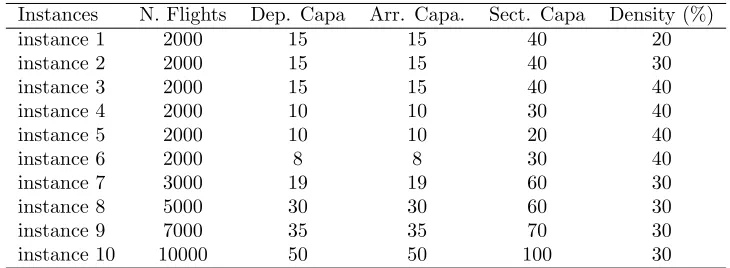
Our computational experiments is conducted on a total of 10 test beds of various sizes and characteristics. The main differences between these test beds are the number of flights (ranging from 2000 to 10 000 flights), the connectivity densities of the networks and the capacities of both the airports and en-route sectors. For each of the instances, there are 20 airports, 48 time periods, which is equivalent to time horizon of 8 hours discretized into time periods of 10 minutes each. There is also a total of 800 waypoints and 300 sectors. The specific characteristics of each of the 10 instances such as the number of flights, the connectivity densities of the networks and the capacities of both the airports and en-route sectors are summarized in Table1.

Table 1. Characteristics of the instances

Instances N. Flights Dep. Capa Arr. Capa. Sect. Capa Density (%)

instance 1 2000 15 15 40 20

instance 2 2000 15 15 40 30

instance 3 2000 15 15 40 40

instance 4 2000 10 10 30 40

instance 5 2000 10 10 20 40

instance 6 2000 8 8 30 40

instance 7 3000 19 19 60 30

instance 8 5000 30 30 60 30

instance 9 7000 35 35 70 30

instance 10 10000 50 50 100 30

Instance 2 and Instance 3 have the same airports and en-route sectors capacities. But the connectivity of the network is 20% for Instance 1, 30% for Instance 2 and 40% for Instance 3. On the other hand, the connectivity of the network for each of Instance 4, Instance 5 and Instance 6 is fixed to 40%, while the capacities of airports and en-route sectors for these instances are being varied. Finally, the other four instances (Instance 7, Instance 8, Instance 9 and Instance 10) have much larger number of flights with the connectivity of each of their networks being fixed to 30%. These are larger instances that allow to test the scalability of our model and solution algorithm.

6.2

Results and analysis

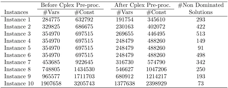
The main focus of our computational experiment was on computing the efficient frontier (set of the non-dominated solutions) for each of our test instances. Some of the important computational characteristics of the instances are reported in Table 2. More precisely, we report in this table, the number of binary variables and constraints before and after the pre-processing procedure embedded in the CPLEX solver, as well as the number of non-dominated solutions found for each of the instances. It is important to point out here that the CPLEX pre-processing is different from the one we presented in Subsection 5.1. This pre-processing uses the constraints of the model to set some variables to their optimum values and discard some constraints when possible. This procedure targets the optimality values of variables and constraints, whereas our pre-processing routine focuses on eliminating variables that do not need to be defined. The results in Table 2 show that before starting the branch-and-cut algorithm for each of the instances, CPLEX is able to reduced about 30% of variables and constraints. It can also be seen that between Instance 1, Instance 2 and Instance 3, higher connectivity of the network yields lager number non-dominated solutions. This may be logic in the sense that higher connectivity implies more options for re-routing the flights and use of different sectors, which in turn may results into a much spread of the delay. On the other hand, the number of non-dominated solutions for Instance 4, Instance 5 and Instance 6 show that the available capacity for either airports or en-route sectors may also impact the number of non-dominated solutions i.e. the scarcer the resources are, the fewer non-dominated solutions there are. This would be a direct result of the fact that the scarcity of resources provides the ATM system with less flexibility for re-routing flights and spread delays across flights in the network.

Table 2. Some output parameters of the instances

Before Cplex Pre-proc. After Cplex Pre-proc. #Non Dominated Instances #Vars #Const #Vars #Const Solutions Instance 1 284775 632792 191754 345610 293 Instance 2 329825 686675 230163 402072 422 Instance 3 354970 697515 269655 446495 513 Instance 4 354970 697515 248479 488260 149

Instance 5 354970 697515 248479 488260 91

The second analysis of our computational experiments is concerned with the trade-offs existing between the three objective functions (2), (3) and (4). The results depicting these trade-offs are shown in Figure3and Figure4. We have chosen heatmap graphics to represent these trade-offs. Other applicable visualization techniques can be found in [41, 42]. Each heatmap has three columns which correspond to the three objective functions. The intensity of the colors vary from 0 to 100 and represents the relative percentage gap of each of the non-dominated solutions. For example, the relative gap of delay in a given non-dominated solution is computed as:

_{delay value of this solution−smallest delay from all the solutions}

largest delay from all the solutions−smallest delay from all the solutions

×100.

Similar calculations are done for the other two objective functions. Therefore, each row of each heatmap corresponds to a non-dominated solution and its color in each column reveals how the corresponding objective function value of this solution compares with the smallest and the largest objective function value among all the non-dominated solutions. As illustration, the bottom row of Figure3ashows that the corresponding solution has the smallest value for delay, the largest value for total deviation from the users’ preferred routes and the smallest value for total ANS route charges.

All the heatmaps in Figure 3 and Figure 4 show that there is not a single row that has the same color for all the three columns simultaneously. This suggests that for all the test instances there is no solution that is able to optimize all the three objective functions simultaneously. One can firstly note that in all the instances, the solutions with good delay values (intensive blue colors in the column of delay) are the ones with the worst costs of deviation (intensive red colors in the column of deviation) and vice-versa. This implies that the total delay of the system cannot be reduced without the preferred trajectories of AUs being distorted and vice-versa. Secondly, it can also be noted that in all the instances, the rows with the intensive blue colors in the column of delay (optimal delay value) also have the intensive blue colors in the ANS route charges column. However, the reverse is not always the case. This means that the solutions that minimize the delay may also minimize the total ANS route charges, while the solutions that minimize the total ANS route charges may result in larger delays for the system. Thirdly, there is also a clear trade-off between the total deviation from the users’ preferred routes and the total ANS route charges. Overall, the heatmaps in Figure3and Figure4show that: i) smaller delays always yield larger values for the deviations from the users’ preferred routes, while the corresponding total ANS route charges; ii) smaller deviations from the users’ preferred routes also yield larger delays and a mix of large and small values for the ANS route charges.

(a) Instance 1 (b) Instance 2

(c) Instance 3 (d) Instance 4

(e) Instance 5 (f) Instance 6

(a) Instance 7 (b) Instance 8

(c) Instance 9 (d) Instance 10

Figure 4. Heat map showing the trade-off between the three objective functions for the larger instances

preferred ones, but this may come at the expense of having routes with longer travel times and slightly larger route charges.

We now describe the efficient solutions for the heatmaps of Instance 4 (Figure 3d), Instance 5 (Figure3e) and Instance 6 (Figure3f). These three instances have similar network connectivity and they only differ with capacities of airports and en-route sectors. It can be seen in Figure3dthat a large number of solutions have delay function values that are fairly far from the optimal value, while nearly half of the solution are within 50% of optimality for the deviation from the users’ preferred routes. However, the total ANS route charges for most of these solutions are very close to optimality. In Figure 3e, the shade of the red color increases for the delay and the deviation from the users’ preferred routes, while it decreases for the total ANS route charges. This shows the kind of impact that reducing the capacity of en-route sectors can have on the network. More precisely, with a reduced capacity of en-route sectors, one should expect higher delays and higher deviations from the users’ preferred routes. However, it does not necessarily imply significant impact on the total ANS route charges, since the trajectories of the flights may end up using the same sectors. Finally, we have in Figure4the heatmaps for larger instances (Instance 7, Instance 8, Instance 9 and Instance 10). These instances have mainly been used to challenge the efficiency of our model and solution approach. Nonetheless, these heatmaps also depict the clear evidence of the existing trade-off between the three objective function of these instances.

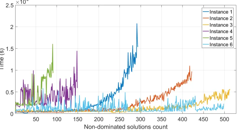
Figure 5. Computational times for instances with 2000 flights

solution of two integer programs. The graphs in Figure5 show for each instance with 2000 flights (Instance 1, Instance 2, Instance 3, Instance 4, Instance 5 and Instance 6) the time needed to compute each of the individual non-dominated solutions. It can be seen in this graph that although these instance all have the same number of flights, airports, sectors and nodes, the computational time for each non-dominated solution varies with the structure of the network. This variation can be located between 400 and 20 000 seconds. However, a vast majority of these solutions are found within 5000 seconds (1.3 hours). A general trend that can be observed from all the instances is that the solution approach requires only about 500 seconds to find the first few non-dominated solutions. The computational time then increases gradually for the other non-dominated solutions. This is clearly because the bounds on the quadrants in the QSM approach get smaller as the non-dominated solutions are found, which renders the feasible sets of the integer programs being solved more or and more restrictive.

Figure 6. Computational times for larger instances

7

Conclusions

In this paper, we have presented a trajectory based mathematical model which aims at optimizing the efficiency of the ATM system under the TBO concept by assigning 4D-trajectories to flights based on the AUs preferences and priorities, and the constraints of the ATM system. The particular aspect of our model is that, not only it considers the complete 4D-trajectories of aircraft, but it also incorporates the preferences and priorities of the ATM stakeholders. The model is formulated as a multi-objective binary optimization problem which considers the preferred 4D-trajectory of all the flights in the pre-tactical planning phase and outputs the entire set of optimal pre-departure 4D-trajectories to be shared or negotiated with other stakeholders and subsequently managed throughout the flight. This set of solution also reflect the trade-offs that exist between the preferences of the ATM stakeholders.

The results of the computational exercise show that our model is capable of handling large scale problems in reasonable amount of time. Furthermore, our model depicts that the efficiency of the ATM system in terms of delay, deviation from the AUs preferred routes and ANS route charges cannot be achieved without compromising some of these KPIs. This shows that our model can provide the basis for a further maturation of the TBO concept and pave the way to a fully integrated performance based air traffic management system. It can also provide a preliminary step towards a full implementation and realization of the collaborative decision making philosophy of the air traffic system.

The proposed approach can support ATFM decisions and can facilitate collaborative decision making at the planning phase. It may be used by the (European) Network Manger in cooperation with all Airspace Users (AUs) to find mutually acceptable solutions that will reflect as close as possible the preferred trajectories of the AUs while ensuring the efficient operation of the entire ATFM system. It is through this process that the TBO objective of providing flexibility to airspace users and ensuring punctuality of the flights is achieved. A multi-criteria, multi-stakeholder framework should be developed in order to analyze the impact of each Pareto optimal solution on individual airlines and flights, and to facilitate the collaborative decision making process. The development of this framework is critical for the deployment of the proposed approach. The development of such a mechanism goes beyond the scope of the current paper and is not free of complexities, among others, how competition between AUs is manifested and in how they strategize in submitting trajectory preferences.

Acknowledgement

This research is part of a project, OptiFrame, that has received funding from the SESAR Joint Undertaking under grant agreement No 699275 under European Unions Horizon 2020 research and innovation program. However, opinions expressed in this work reflect the authors’ views only and SESAR and/or EUROCONTROL shall not be considered liable for them or for any use that maybe made of the information contained herein.

References

[1] SESAR (2015), The roadmap for delivering high performing aviation for Europe. Eu-ropean ATM Master Plan. Executive view. Edition 2015.

[2] EUROCONTROL (2013), Challenges of growth 2013: Summary re-port. www.eurocontrol.int/sites/default/files/content/documents/ official-documents/reports/201307-challenges-of-growth-summary-report. pdf

[3] SESAR (2009), SESAR Concept of Operations Step 1. D65-011. Project B4.2.

[4] O. T. Pleter, C. E. Constantinescu & I. B. Stefanescu (2009), Objective function for 4D trajectory optimization in Trajectory Based Operations. AIAA Guidance, Navigation, and Control Conference, 10–13 August 2009, Chicago, Illinois.

[5] C. Wynnyk, M. Balakrishna, P. MacWilliams & T. Becher (2013), 2011 Trajectory Based Operations Flight Trials. Tenth USA/Europe Air Traffic Management Research and Development Seminar (ATM2013). 10–13 June 2013, Chicago, Illinois.

[6] A. R. Odoni (1987), The flow management problem in air traffic control.in A. R. Odoni, L. Bianco & G. Szegoeds. Flow Control of Congested Networks, Springer-Verlag, Berlin, 269–288.

[8] K. Lindsay, E. Boyd & R. Burlingame (1993), Traffic flow management modelling with the time assignment model.Air Traffic Control Quarterly, 1 (3), 255–276.

[9] D. Bertsimas & S. Stock Patterson(1998) The air traffic management problem with en-route capacities.Operations Research, 46, 406–422.

[10] D. Bertsimas & S. Stock Patterson (2000), The traffic flow management rerouting problem in air traffic control: a dynamic network flow approach.Transportation Science, 34, 239–255.

[11] D. Bertsimas, G. Lulli & A. Odoni (2011), An integer optimization approach to large-scale air traffic flow management.Operations Research, 59(1), 211–227.

[12] A. Agust´ın, A. Alonso-Ayuso, L.F. Escudero & C. Pizarro (2012), On air traffic flow management with rerouting. Part I: Deterministic case. European Journal of Opera-tional Research, 219, 156–166.

[13] A. M. Churchill, D. J. Lovell & M. O. Ball (2009), Evaluating a new formulation for large-scale traffic flow management. Eighth USA/Europe Air Traffic Management Research and Development Seminar (ATM2009). Napa, California USA June 29–July 2, 2009.

[14] F. Djeumou Fomeni, G. Lulli & K. Zografos (2017), An optimization model for assigning 4D-trajectories to flights under the TBO concept. Twelfth USA/Europe Air Traffic Management Research and Development Seminar (ATM2017). Seattle, Washington, USA June 26-30, 2017.

[15] The OptiFrame Consortium (2016), Technical report reviewing the state-of-the-art on ATFM. D7. SESAR exploratory Research. Available upon request. www. lancaster. ac. uk/ lums/ central/ current-projects/ optiframe/.

[16] V. Dal Sasso, F. Djeumou Fomeni, G. Lulli, G. Murgese, & K. Zografos (2018), A Multi-Objective Integer Approach for Optimizing Trajectory Based Operations (TBO).

Annual Meeting of the Transportation Research Board (TRB). Washington, D.C, United States January 7–11, 2018.

[17] E. W. Dijkstra (1959), A note on two problems in connexion with graphs.Numerische Mathematik, 1, 269–271.

[18] H. D. Sherali, J. C. Smith & A. A. Trani (2002), An airspace planning model for selecting flight-plans under workload, safety, and equity considerations.Transportation Science, 36(4), 378–397.

[19] A. Kim & M. Hansen (2013), A framework for the assessment of collaborative en route resource allocation strategies.Transportation Research Part C, 33, 324–339.

[20] N. Pilon, S. Ruiz, A. Bujor, A. Cook & L. Castelli (2016), Improved flexibility and equity for airspace users during demand-capacity imbalance. In D. Schaefer (Editor) Proceedings of the SESAR Innovation Days (2016) EUROCONTROL. ISSN 0770-1268.

[22] SESAR, D07 UDPP Step 2 V1, Project 07.06.04, Ed. 00.02.02, January 2014.

[23] A. Jacquillat, A. R. Odoni & M. D. Webster (2016), Dynamic control of runway con-figurations and of arrival and departure service rates at JFK airport under stochastic queue conditions.Transportation Science, 51 (1), 155–176.

[24] A. Cook (2007), European air traffic management: princple, practice and research. Ashgate, Aldershot. ISBN 9780754672951.

[25] IBM ILOG CPLEX Optimization Studio www-01.ibm.com/software/commerce/ optimization/cplex-optimizer/.

[26] Matlab R2015a-academy use https://uk.mathworks.com/products/new_products/ release2015a.html.

[27] GCC, the GNU Compiler Collection version 4.8.1https://gcc.gnu.org/.

[28] The OptiFrame Consortium (2016), Report of the OptiFRAME workshop: the stakeholders views. October 5, 2016, Brussels. Available upon request. http://www. lancaster.ac.uk/lums/central/current-projects/optiframe/.

[29] The OptiFrame Consortium (2017), OptiFrame computational framework. D11. SESAR exploratory Research. Available upon request.www. lancaster. ac. uk/ lums/ central/ current-projects/ optiframe/.

[30] EUROCONTROL, The Central Route Charges Office and the Route Charges System.

www. eurocontrol. int/ articles/ establishing-route-charges

[31] International Civil Aviation Organization-ICAO ATMRPP (2015), The TBO concept. Version Appendix A to WP652-TBOCD 3.0. www. icao. int/ Meetings/ anconf12/ Document% 20Archive/ 9854_ cons_ en[ 1] .pdf

[32] International Civil Aviation Organization-ICAO (2005), Global air traffic management operational concept. First edition-2005. www. sesarju. eu/ sites/ default/ files/ documents/ reports/ Appendix_ A_ to_ WP652_ TBOCD_ 3. 0. pdf

[33] ICAO Document 4444 ATM/501 (2001), Procedures for air navigation services- Air Traffic Management.International Civil Aviation Organization

[34] N. Boland, H. Charkhgard & M. Savelsbergh (2017), The quadrant shrinking method: a simple and efficient algorithm for solving tri-objective integer programs. European Journal of Operational Research, 260, 873–885.

[35] J. Sylva, & A. Crema (2004), A method for finding the set of non-dominated vectors for multiple objective integer linear programs.European Journal of Operational Research, 158, 46–55.

[36] M. ¨Ozlen, B. A. Burton & C. A. MacRae (2013), Multi-objective integer program- ming: An improved recursive algorithm. Journal of Optimization Theory and Applications, 160, 470–482.

[38] N. Boland, H. Charkhgard & M. Savelsbergh (2016), The L-shape search method for triobjective integer programming. Mathematical Programming Computation, 8, 217– 251.

[39] G. Chiandussi, M. Codegone, S. Ferrero & F. E. Varesio (2012), Comparison of multi-objective optimization methodologies for engineering applications.Computers & Math-ematics with Applications, 63(5), 912–942.

[40] J. Cohon (1978), Multiobjective programming and planning.Academic Press Inc. Lon-don.

[41] A. Pryke, S. Mostaghim & A. Nazemi (2007), Heatmap Visualization of Population Based Multi Objective Algorithms.In: S. Obayashi, K. Deb, C. Poloni, T. Hiroyasu & T. Murata (eds) Evolutionary Multi-Criterion Optimization. EMO 2007. Lecture Notes in Computer Science, vol 4403. Springer, Berlin, Heidelberg, pp 361–375.

[42] T. Tuˇsar & B. Filipiˇc (2015), Visualization of Pareto Front Approximations in Evolu-tionary Multiobjective Optimization: A Critical Review and the Prosection Method.