Steady State Simulation of 33 kV Power Grid

ISSN Online: 2327-5901 ISSN Print: 2327-588X

Steady State Simulation of 33 kV Power Grid

Kiu Han Teck, Nader Barsoum

Electrical and Electronics Engineering, University Malaysia Sabah, Kota Kinabalu, Malaysia

Abstract

An example is presented in this paper relating to power problems in Sandakan power network. Sandakan is a suburb in east coast of Sabah state of Malaysia. The problems were reported with power flow and N-1 contingency in terms of blackout after main grid supply outages with overload and high fault current on distribution system. This paper focuses on analysis of steady state stability of 33 kV power grid using load flow, contingency analysis and voltage stability (P-V Curve). The analysis is done by using industrial grade power software called Power System Simulation for Engineers (PSS/E). The power flow result showed that there are three generators generating out of limits. Contingency results showed that three transformer branches and three distribution branches are affected. There are nine weakest buses that violate contingency voltage deviation criterion and cannot withstand more load power when N-1-1 case in the branch of bus 8 to bus 28 is under outage.

Keywords

Load Flow, Contingency Analysis, PV Curve, Voltage Stability, Overload, Voltage Deviation Violation

1. Introduction

In Sabah grid, the power demand is increasing annually but the generated capac-ities is less than the power demand, especially in the east coast [1]. The current equipments in transmission system such as electricity cable are getting old and are found operated closer to their limits of stability and cannot withstand with increased power supply [2]. Due to these, the grid system is exposed to distur-bances or contingencies which can cause system collapse and blackout. Sabah faced two major serious blackouts [1]. The most severe blackout happened in 2014 for 10 hours of state-wide blackout. The collapse is triggered by flashover which is from conductor of 132 KV transmission line. Another one is blackout in the whole east coast due to outage of 275 KV transmission line.

How to cite this paper: Teck, K.H. and Barsoum, N. (2018) Steady State Simulation of 33 kV Power Grid. Journal of Power and Energy Engineering, 6, 106-124.

https://doi.org/10.4236/jpee.2018.66007

Received: May 31, 2018 Accepted: June 26, 2018 Published: June 29, 2018

Copyright © 2018 by authors and Scientific Research Publishing Inc. This work is licensed under the Creative Commons Attribution International License (CC BY 4.0).

http://creativecommons.org/licenses/by/4.0/ Open Access

As stated in Sabah grid Code [3], most of transmission lines, distribution and transformers fulfil N-1 contingency requirement, but in fact studies showed that there is no N-1 contingency in aging existing transformer and existing line con-figuration [2]. Therefore, when N-1 contingency happens, overload conditions occur on those transformers, distribution and transmission lines.

Contingency analysis has been developed by [4] using sensitivity factors to approximate power flow on branches whereas voltage performance index is used by [5] to approximate the contingency voltage on a certain bus in a power sys-tem. For voltage stability part, [6] reviewed four commonly used voltage stability analysis tools which are PV/QV curve analysis, L index, Modal analysis and V/Vo index. Authors have done comparison of accuracy results on IEEE bus power system.

This paper focuses on steady state stability for distribution level of power grid. Thus, 33 KV Sandakan network of Sabah Grid System is chosen to simulate steady state stability which consists of load flow simulation, contingency simula-tion and P-V curve. Contingency scenarios are created to test its overall steady state stability of the grid in terms of contingency voltage deviation violation and percentage overload. Moreover, P-V analysis is performed to determine the weakest buses in the network. The process of analysing the stability can be daunting and challenging if the power network is highly complex, large size and non-linear. The process takes a lot of time in the calculations to access all the power variables and contingencies [7]. Therefore, a Power System Simulation for Engineers (PSS/E) software is utilized to perform all power flow computations in this steady state analysis.

2. Existing N-1 Network

The existing model of power system network shown in Figure 1 is modelled by using (PSS/E).This network is disconnected from the main grid power supply, especially the supply from 275 KV transmission line. Therefore, in that case, the network itself is assumed as N-1 under outages of main grid and is considered as external N-1 condition. Date of bus names, Transformers, generators, loads and branches regarding powers and impedances are given in the tables at the Ap-pendix.

The grid system has the following major components: 1) Buses: 34 (27 of them are connected)

2) Loads: 24 (22 of them are in service)

3) Branches: 40 (29 out of 32 distribution branches and 8 transformer branches are in service)

4) Fixed shunts: 6 (5 of them are in service)

5) Generators (machines): 8 (6 of them are in service)

3. Load Flow Analysis

Load flow analysis is used to calculate voltage, current flows, active and reactive

Figure 1. Existing power network drawn in PSS/E.

powers, power losses for generators, load and generator buses, distribution and transformer branches, and loads in the Power network. There are two types of solutions in PSS/E: Newton Raphson and Gauss Seidel load flows. Due to com-plexity and large number of buses in N-1 power network, Newton Raphson is chosen due to faster converging rate and repetitive complicated computation of Jacobian matrix and its minimal sensitivity. For contingency cases, Fixed Slope Decoupled load flow which is part of Newton Raphson created by Siemens Company is chosen as it performs better in difficult and complicated cases

compared to other types of methods.

There are four power elements that load flow used to calculate. These are: 1) Generators (swing buses): generated active and reactive power flows 2) Distribution and transformer branches: current flows, active and reactive power flows, percentage voltage drop, power factor, and power losses.

3) Buses (load buses and generator buses): bus voltage, active and reactive power flows, and current flows.

4) Loads: active and reactive power flows, current flows, and percentage load-ing.

Table 1 shows the power flow results of generated active power and reactive power for each in-service generating unit which act as swing bus. Pmax and Pmin

are the maximum and minimum generated capacity for each generator. Same goes to Qmin and Qmax which represent reactive power capacity. With respect to

PGen, all generators generated within their active power and reactive power lim-its except for generators named KB_6.6, SB_6.6, and BN_11.

Table 2 shows the total generated power by all generators before and after the

Table 1. Generators results.

Bus No. Bus Name Base kV PGen _(MW) Pmax

(MW) (MW) Pmin (MVAr) QGen (MVAr) Qmax (MVAr) Qmin

1 KB_6.6 6.6000 24.6 10.0 0.0 5.9 7.3 0.5

2 SB_6.6 6.6000 25.0 10.0 0.0 8.1 7.3 0.5

23 GN_11 11.000 5.0 37.0 20.0 1.6 24.8 −14.7

28 BN_11 11.000 27.3 20.0 0.0 12.1 21.2 −15.2

29 LD1_11 11.000 7.6 15.0 8.0 2.6 11.4 −8.5

32 LD2_11 11.000 7.6 15.0 8.0 2.6 11.4 −8.5

33 LD3_11 11.000 7.5 15.0 8.0 1.6 11.4 −8.5

34 LD4_11 11.000 7.5 15.0 8.0 1.6 11.4 −8.5

Table 2. Total generated power in sandakan before and after N-1 outage.

Bus No. Bus Name Base kV _{(After Outage)} PGen (MW) _{(Before Outage)} PGen (MW) _{Capacity (MW)} Active Power

1 KB_6.6 6.6000 24.6 10.00 10.0

2 SB_6.6 6.6000 25.0 10.00 10.0

23 GN_11 11.000 5.0 14.76 37.0

28 BN_11 11.000 27.3 15.00 20.0

29 LD1_11 11.000 7.6 9.50 15.0

32 LD2_11 11.000 7.6 9.50 15.0

33 LD3_11 11.000 7.5 15.00 15.0

34 LD4_11 11.000 7.5 15.00 15.0

TOTAL 112.10 98.76 137.00

main supply outage from 275 KV transmission line with respect to the total gen-erated capacity. The table shows that the power demand increase by 13.34 MW from 98.76 MW after the outage, but they are within the total generated capacity.

Table 3 shows the load flow results for all in-service branches (transformer and distribution). Note: DB is distribution branch, TB is transformer branch. Transformer branches are found higher active and reactive power losses, higher percent of voltage drop, higher current flows and higher active and reactive power flows than that in distribution branches. Only transformer branches have higher loadings problem compared to distribution branches. For distribution branches, DB10_1 is recorded with highest power losses. For transformer branches, TB3 is recorded with highest reactive power loss and TB5 and TB6 share the highest active power losses. TB2 is recorded with highest percent of voltage drop among all branches, followed by DB2_1 and DB2_2. DB14_1, DB14_2, DB17_1 and DB17_2 are recorded with zero among all variables.

Table 4 and Table 5 show the load flow results for all in-service buses. Load buses are represented by bus code 1 while generator buses are represented by bus code 2. UB_33 and BM_33 are recoded zero in active and reactive power flows and current flows due to no loads connected to them. Generator buses are rec-orded higher current flows compared to load buses. All bus voltages are within contingency voltage range stated by Distribution Code of Energy Commission. The voltage range is from 0.9 pu to 1.1pu. That means all bus voltages are safe and secure under N-1 case which is disconnected from main grid supply.

This load flow analysis shows that all bus voltages are slightly higher than 100% and 2 load buses are overloaded as well as 3 generators generating out of limits.

4. Contingency Analysis

To compute the branch power flows after certain level of outage, contingency sensitivity factors are used to approximate the change in line flows and the changes in generation in a power system. It is one of fastest way to calculate possible overloads in a power system network. The main two sensitivity factors are Generation Shift Factors (GSF) and Line Outage Distribution Factors (LODF).

For GSF part, the generation factor is defined as changes in power flow in par-ticular line when a change in power generation at reference bus occurs.

Generation shift factors,

l li

Gi

PF P

α =∆

∆

where ∆PFl = changes in power flow on lth line Gi

P

∆ _{= changes in generation which takes place on i}th _bus

For LODF, the line outage distribution factor is defined as the change in pow-er flow on ith _{line during pre-contingency line flow on 𝑙𝑙}th _line.

Line outage distribution factors,

Table 3. Distribution and transformer branch results.

Branches MW Flows MVAr Flows % Voltage Drop kW Losses kVAr Losses

DB1_1 13.606 3.741 0 0.002 0.196

DB1_2 13.3 1.644 0 0.002 0.176

DB2_1 12.004 6.544 2.25 30.998 557

DB2_2 12.004 6.544 2.25 30.998 557

DB3 13.752 7.036 0 0.002 0.234

DB4_1 7.457 0.646 0.22 13.641 36.767

DB4_2 7.457 0.646 0.22 13.641 36.767

DB5_1 9.328 4.194 0.95 11.233 195

DB5_2 9.328 4.194 0.95 11.233 195

DB6_1 13.406 1.646 0.75 35.109 632

DB6_2 13.406 1.646 0.75 35.109 632

DB7_1 6.187 −3.415 0.08 9.547 29.333

DB7_2 6.187 −3.415 0.08 9.547 29.333

DB8_1 6.225 −3.339 0.05 27.673 47.071

DB8_2 6.225 −3.339 0.05 27.673 47.071

DB9_1 6.907 −1.432 0.08 9.47 15.861

DB9_2 6.907 −1.432 0.08 9.47 15.861

DB10_1 12.132 −5.175 0.07 83.315 225

DB11_1 9.181 −3.916 0.04 30.672 82.668

DB12_1 22.751 2.229 0.09 16.57 34.142

DB12_2 22.751 2.229 0.09 16.57 34.142

DB13_1 9.212 −3.833 0.03 32.376 87.261

DB14_1 0 0 0 0 0

DB14_2 0 0 0 0 0

DB15_1 10.072 4.878 0 0.001 0.123

DB16_1 9.423 4.565 0.01 0.393 1.058

DB16_2 9.423 4.565 0.01 0.393 1.058

DB17_1 0 0 0 0 0

DB17_2 0 0 0 0 0

TB1 13.368 2.902 2.09 67.639 1258

TB2 13.68 5.136 3.59 74.983 1395

TB3 26.747 9.69 3.8 29.418 3530

TB4 12.879 1.094 0.76 49.758 925

TB5 11.549 2.247 1.65 81.776 629

TB6 11.549 2.247 1.65 81.776 629

TB7 11.361 1.21 1.15 77.846 599

TB8 11.361 1.21 1.15 77.846 599

Table 4. Load flows results for all in-service buses.

Buses Bus Code Bus Voltage (pu) MW Loading MVAr Loading Amp Loading

BM_33 1 1.0316 0 0 0

BN_11 2 1.049 26.747 9.69 1423

BS_33 1 1.011 26.718 12.293 508.9

GN_11 2 1.04 12.879 1.094 652.3

KB_6.6 2 1.03 13.368 2.902 1162

KB_33 1 1.0091 13.3 1.644 232.4

KG_33 1 1.0329 12.394 6.772 239.2

LD1_11 2 1.049 11.549 2.247 588.7

LD2_11 2 1.049 11.549 2.247 588.7

LD3_11 2 1.044 11.361 1.21 574.4

LD4_11 2 1.044 11.361 1.21 574.4

LD_33 1 1.0337 12.375 12.823 301.6

LK_33 1 1.009 18.845 9.127 363.1

LP_33 1 1.0325 45.501 4.459 774.7

MS_33 1 1.0316 13.796 9.578 284.8

PI_33 1 1.0324 34.143 12.907 618.6

SA_33 1 1.0316 45.468 13.087 802.4

SB_3.3 1 1.0091 13.606 3.741 244.6

SB_6.6 2 1.045 13.68 5.136 1223

SC_33 1 1.032 9.212 3.833 169.2

SD2_33 1 1.0091 45.658 12.421 820.4

SD_33 1 1.0091 23.946 11.973 464.2

SM_33 1 0.9993 14.887 7.21 289.6

SR_33 1 1.009 10.072 4.878 194

TS_33 1 1.0016 45.375 16.043 840.7

UB_33 1 1.032 0 0 0

l

li o

i

PF d

P

∆

= ₍₂₎

where ∆PFl = changes in power flow on 𝑙𝑙th line o

i

P = Power line flow on ith _{line before contingency of i}th _line

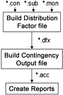
In PSS/E software, the process of performing contingency analysis is done automatically and comprehensively without manually tripping each line. Before carrying out N-1 contingency analysis, three types of files are created. They are *mon.file, *sub.file and *con.file. Each file is described in Table 6. Figure 2

shows the process of creating these files.

Table 5. Load flow results for all in-service loads.

Load Buses Id MW Flows (kW) MVAr Flows (kVAr) Current Flows % PF % Loading

SD_33 1 2573 1246 49.57 90 99.1

SD_33 2 2879 1395 55.47 89.99 99.1

SD_33 3 4460 2160 85.92 90 99.1

SD_33 4 282 136 5.428 90.07 99.1

TS_33 1 17,289 8373 335.6 90 99.8

TS_33 2 13,172 6379 255.7 90 99.8

SM_33 1 10,415 5044 202.6 90 100.1

SM_33 2 4472 2166 86.99 90 100.1

BS_33 1 2181 1056 41.93 90 98.9

BS_33 2 5881 2848 113.1 90 98.9

LD_33 1 6849 3317 128.8 90 96.7

LD_33 2 5526 2676 103.9 90 96.7

PI_33 1 4497 2178 84.68 90 96.9

PI_33 2 3382 1638 63.68 90 96.9

MS_33 1 6947 3365 130.9 90 96.9

MS_33 2 6849 3317 129.1 90 96.9

SR_33 1 4031 1952 77.66 90 99.1

SR_33 2 6041 2926 116.4 90 99.1

LK_33 1 5416 2623 104.3 90 99.1

LK_33 2 3357 1626 64.68 90 99.1

SD2_33 1 −5000 0 86.69 100 99.1

TS_33 1 0 −6019 105.1 0 −

SM_33 1 0 −5992 104.9 0 −

BS_33 1 0 −6133 106.1 0 −

LD_33 1 0 −12823 217 0 −

PI_33 3 0 −3197 54.18 0 −

MS_33 3 0 −9578 162.4 0 −

Table 6. Three types of PSS/E files with descriptions.

File Type Description

*mon.file It informs load flow simulator the branches needed to be monitored when N-1 contingency happens. It also monitors and records the bus voltages within specific ranges or outside the range.

*sub.file It tells load flow analysis to consider and perform at specific zone. It includes all _{involved power network elements in the case study.}

*con.file It is used to trip line or power elements to create contingency scenarios. Three types of contingencies: N-0 (system intact), N-1 (single power element outage) and N-2 (two power elements outage). In this case, N-1 is chosen.

Figure 2. Process of creating these files.

Before doing any N-1 contingency analysis, it is compulsory to comply the contingency voltage range is set within ±10% of nominal voltage at steady state level for 33 kV distribution network. Since the nominal voltage is 1.0 pu, there-fore the range is from 0.9 pu to 1.1pu. Besides, there are two types of contingen-cy case analyzed as follows:

1) External contingency (N-1): is the power network cut off supply from main grid

2) Internal contingency (N-1-1): is another contingency happens after exter-nal contingency occurred

Branch flows and overload condition are determined for affected branches in every contingency case. Also, determines the buses that violate the contingency voltage deviation criterion which is the changes in voltage cannot rise more than 0.06 pu and drop more than 0.03 pu.

From Table 7, transformer branches which are marked in italic are recorded higher than that in distribution branches. The most severe overload cases hap-pen on the transformer branches near to SB_6.6 and KB_6.6 generators. This is because the lost generation from incomer main grid is supplied by these two supplies, causing them to generate more power demand.

In the contingency analysis, all branches except six branches are considered safe and remained unaffected throughout all contingency cases (N-1-1 and N-1).

Table 8 shows that the list of 31 unaffected branches out of 37 branches involved in contingency analysis. The branches highlighted in italic are transformer branches and the rest are distribution branches.

There is no contingency voltage deviation violation report in all contingency cases except for case when outage of transformer branch bus 8 to bus 28. The bus that cannot withstand N-1 or N-1-1 is if they violate the voltage deviation criterion. The violation case can be shown visually in Figure 3. The affected buses highlighted in red are the buses that cannot withstand N-1. The transfor-mer branch outage is highlighted in black. Table 9 shows the affected buses during the contingency case named SINGLE 8-28 with their respective contin-gency voltage, initial voltage, and the voltage deviation limits.

Table 7. List of affected branches with respective total number of involved cases and overload percent.

Affected Branches

No. of Cases Involved

from Total 38 contingency Cases Overload Percent Ranges (%)

From Bus To Bus

Id

No Name No Name

1 KB_6.6 4 KB_33 1 38 174.0 - 228.1

2 SB_6.6 3 SB_33 1 38 173.4 - 238.3

6 TS_33 8 BS_33 2 1 110.2

8 BS_33 28 BN_11 1 38 110.5 - 142.0

14 SA_33 16 LP_33 1 8 101.8 - 165.0

14 SA_33 16 LP_33 2 8 101.8 - 165.0

Figure 3. N-1-1 case with affected buses when outage of transformer branch from bus 8 to bus 28.

Table 8. List of unaffected branches throughout all contingency cases (N-1 and N-1-1 cases).

Unaffected Branches

From Bus To Bus

Id

No. Name No. Name

16 LP_33 29 LD1_11 1

16 LP_33 32 LD2_11 1

16 LP_33 33 LD3_11 1

16 LP_33 34 LD4_11 1

11 PI_33 23 GN_11 1

3 SB_33 26 SD2_33 1

4 KB_33 26 SD2_33 2

5 SD_33 14 SA_33 1

5 SD_33 14 SA_33 2

5 SD_33 26 SD2_33 1

6 TS_33 7 SM_33 1

6 TS_33 7 SM_33 2

6 TS_33 8 BS_33 1

6 TS_33 8 BS_33 2

6 TS_33 26 SD2_33 1

6 TS_33 26 SD2_33 2

9 KG_33 10 LD_33 1

9 KG_33 10 LD_33 2

9 KG_33 11 PI_33 1

9 KG_33 11 PI_33 2

11 PI_33 12 MS_33 1

11 PI_33 12 MS_33 2

11 PI_33 14 SA_33 1

11 PI_33 18 SC_33 1

14 SA_33 16 LP_33 1

14 SA_33 16 LP_33 2

14 SA_33 18 SC_33 1

14 SA_33 20 BM_33 1

14 SA_33 20 BM_33 2

15 SR_33 17 LK_33 1

17 LK_33 26 SD2_33 1

17 LK_33 26 SD2_33 2

18 SC_33 19 UB_33 1

18 SC_33 19 UB_33 2

Contingency results showed 3 transformer branches and 2 distribution branches are affected.

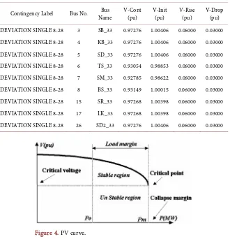
5. P-V (Load Power-Load Voltage) Curve Analysis

P-V curve is commonly used as voltage stability analysis tool to analyze maxi-mum additional load power that a bus can sustain before its voltage collapses, after the load power exceeds its power limits. Figure 4 shows a simple P-V curve. When load power exceeds the power limit of a bus, the bus voltage will start to drop until reaching the critical point, which is voltage collapse point when the bus reaches the maximum additional power. PSS/E is able to simulate different P-V curve for different level of contingency. So, in this paper, P-V curve is simulated for external contingency and internal contingency cases for all 26 in-service buses. The maximum additional power transfer and voltage col-lapse point are recorded for each buses in every contingency cases.

All buses are simulated with P-V curves for every contingency case. Thus, 988 (38 contingency cases X 26 buses) P-V curves are simulated. Table 10 shows the list of number of contingency cases with the overall maximum additional power transfer among all buses. Among 38 contingency cases, 15 of them are recorded with the highest maximum additional power transfer with 312.50 MW, followed

Table 9. Contingency voltage deviation violation reports.

Contingency Label Bus No. _Name Bus V-Cont _(pu) V-Init _(pu) V-Rise _(pu) V-Drop _(pu)

DEVIATION SINGLE 8-28 3 SB_33 0.97276 1.00406 0.06000 0.03000

DEVIATION SINGLE 8-28 4 KB_33 0.97276 1.00406 0.06000 0.03000

DEVIATION SINGLE 8-28 5 SD_33 0.97276 1.00406 0.06000 0.03000

DEVIATION SINGLE 8-28 6 TS_33 0.93054 0.98853 0.06000 0.03000

DEVIATION SINGLE 8-28 7 SM_33 0.92785 0.98622 0.06000 0.03000

DEVIATION SINGLE 8-28 8 BS_33 0.93149 1.00015 0.06000 0.03000

DEVIATION SINGLE 8-28 15 SR_33 0.97268 1.00398 0.06000 0.03000

DEVIATION SINGLE 8-28 17 LK_33 0.97268 1.00398 0.06000 0.03000

DEVIATION SINGLE 8-28 26 SD2_33 0.97276 1.00406 0.06000 0.03000

Figure 4. PV curve.

by 6 cases with 306.25 MW and 5 cases with 287.50 MW. The only one case with the lowest maximum additional power transfer (143.75 MW) happened when outage of transformer branch from bus 8 to bus 28. That means all buses can only withstand incremental power transfer up to 143.75 MW when this outage happens. That is why this case has only voltage violation cases, referring to

Table 8. They cannot withstand higher power flows compared to other cases. Among all P-V curves, almost all buses except generator buses have their vol-tage collapse point at below 0.9 pu. That is not reasonable that the steady state operating voltage is within 10% of the nominal voltage, from 0.9 pu to 1.1 pu. Since the weakest case is SINGLE 8-28 (1), in order to determine weakest buses, the maximum incremental power transfer at 0.9 pu of the nominal voltage is de-termined for each bus. Any voltage which is outside of the tolerance is not ac-ceptable. Figure 5 shows the finding of maximum additional power transfer at

Table 10. List of number of contingency cases and the maximum additional power transfer.

No. of contingency cases Maximum Additional Power Transfer (MW)

1 143.75

1 218.75

2 243.75

4 256.25

2 268.75

5 287.50

2 293.75

6 306.25

15 312.50

Figure 5. Maximum additional power transfer at 0.9 pu in PV curve.

0.9 pu. Table 11 shows the maximum additional power transfer at 0.9 pu for each bus with respective voltage collapse point at contingency case named SINGLE 8-28.

From Table 11, the generator buses (KB_6.6, SB_6.6, BN_11, GN_11, LD1_11, LD2_11, LD3_11 and LD4_11) have maintained constant bus voltage along all incremental power transfer. This is because no losses involved when the generators generate the output voltage to the nearest buses. The loss will be very small. Any bus that withstand below 50% of the 143.75 MW is considered as weakest buses. Therefore, the weakest buses are SB_33, KB_33, SD_33, TS_33,

Table 11. List of all buses with their respective maximum additional power transfer at 0.9

puin weakest contingency case (Single 8-28).

Bus No. Bus Name Maximum Incremental Power Flow _{(MW) at 0.9 pu} Voltage Collapse _{Point (pu)}

1 KB_6.6 143.75 1.030

2 SB_6.6 143.75 1.045

9 KG_33 80 0.812

10 LD_33 80 0.807

11 PI_33 83 0.827

12 MS_33 86 0.821

14 SA_33 92 0.843

28 BN_11 143.75 1.049

29 LD1_11 143.75 1.049

32 LD2_11 143.75 1.049

33 LD3_11 143.75 1.044

34 LD4_11 143.75 1.044

18 SC_33 91 0.834

19 UB_33 91 0.834

20 BM_33 92 0.843

23 GN_11 143.75 1.040

16 LP_33 98 0.850

3 SB_33 26 0.618

4 KB_33 26 0.618

5 SD_33 26 0.618

6 TS_33 8 0.349

7 SM_33 6 0.334

8 BS_33 8 0.333

15 SR_33 29 0.618

17 LK_33 29 0.618

26 SD2_33 27 0.618

SM_33, BS_33, SR_33, LK_33, and SD2_33. The results from P-V actually corre-late with the Contingency Voltage Violation results shown in Table 9.

6. Conclusions

Sandakan power network has serious overload condition on generating units compared to other distribution lines. This paper shows that 3 generators out of 8 are generating out of the limits. For all loads, a vast majority of loads are margi-nally overload. There are 9 weakest buses determined at weakest N-1-1 contin-gency case via P-V curve and Contincontin-gency analysis. The buses are found dropped out of the contingency voltage deviation criterion and can withstand smaller power transfer after the power exceeds their bus power limit.

Contingency analysis is a very important and useful tool in planning the un-planned electrical outages. It can predict the future power system conditions under outages. It evaluates how many those buses survive under outages and those didn’t. In this case, PSS/E is able to perform contingency analysis within seconds and provide with accurate results. To improve its stability, two types of FACTS devices are recommended: UPFC and STATCOM. UPFC is used to compensate power flows to reduce overload condition whereas STATCOM is used to maintain bus voltage for better voltage profile.

References

[1] (2015) Sabah Electricity Outlook 2015. Energy Commission Malaysia, 1-60. [2] Songkin, M., Barsoum, N.N., Wong, F. and Lim, P.Y. (2017) A Study on Sabah Grid

System Stability. 2017 IEEE 2nd International Conference on Automatic Control and Intelligent Systems (I2CACIS 2017), 207-212.

[3] Grid Code for Sabah and Labuan (Amendments) 2017 (2017) Energy Commission Malaysia (Suruhanjaya Tenaga Malaysia). 1-206.

[4] Satyanarayana, B., Deepak, J. and Khyati, D. (2016) Contingency Analysis of Power System by Using Voltage and Active Power Performance Index. 1st IEEE Interna-tional Conference on Power Electronics, Intelligent Control and Energy Systems

(ICPEICES), 1-5.

[5] Roman, V. and Lucie, N. (2015) Sensitivity Factors for Contingency Analysis. Insti-tute of Electrical and Electronics Engineering (IEEE), 1-5.

[6] Reis, C., Andrade, A. and Maciel, F.P. (2009) Voltage Stability Analysis of Electrical Power System. Institute of Electrical and Electronics Engineering (IEEE), 244-248. [7] Barsoum, N., Asok, C.B., SzuKwong, D.T. and Kit, C.G.T. (2017) Effect of Distri-buted Generators on Stability in a limited bus Power Grid System. Journal of Power and Energy Engineering, Scientific Research Publishing, 5, 74-91.

Appendix

Table A1. Buses Data Used in PSS/E.

Bus No. Bus Name Bus Code Base kV Voltage (pu) Angle (deg)

1 KB_6.6 −2 6.6 1.0085 −15.28

2 SB_6.6 −2 6.6 1.0085 −15.28

3 SB_33 1 33.0 0.9594 −19.51

4 KB_33 1 33.0 0.9594 −19.51

5 SD_33 1 33.0 0.9594 −19.51

6 TS_33 1 33.0 0.9524 −23.99

7 SM_33 1 33.0 0.9499 −24.28

8 BS_33 1 33.0 0.9709 −23.60

9 KG_33 1 33.0 0.9543 −25.46

10 LD_33 1 33.0 0.9545 −25.73

11 PI_33 1 33.0 0.9549 −24.88

12 MS_33 1 33.0 0.9538 −25.07

13 TR_33 4 33.0 1.0000 0.00

14 SA_33 1 33.0 0.9615 −23.11

15 SR_33 1 33.0 0.9593 −19.52

16 LP_33 1 33.0 0.9615 −23.11

17 LK_33 1 33.0 0.9593 −19.52

18 SC_33 1 33.0 0.9580 −24.01

19 UB_33 1 33.0 0.9580 −24.01

20 BM_33 1 33.0 0.9615 −23.11

21 SI_33 4 33.0 1.0000 0.00

22 KG_11 4 11.0 1.0000 0.00

23 GN_11 2 11.0 0.9549 −54.88

24 SG2_11 4 11.0 1.0000 0.00

25 SG1_11 4 11.0 1.0000 0.00

26 SD2_33 1 33.0 0.9594 −19.51

27 BS_33 4 33.0 1.0000 0.00

28 BN_11 2 11.0 1.0490 10.42

29 LD1_11 2 11.0 0.9615 −23.11

30 BG_33 4 33.0 1.0000 0.00

31 B8_11 4 11.0 1.0000 0.00

32 LD2_11 2 11.0 0.9615 −23.11

33 LD3_11 2 11.0 0.9615 −23.11

34 LD4_11 2 11.0 0.9615 −23.11

Table A2. Transformer branch data used in PSS/E.

Transformer Branches

Tap

Positions MVA Base Winding

From Bus To Bus

Id

No Name No Name

1 KB_6.6 4 KB_33 1 8 14.0

2 SB_6.6 3 SB_33 1 8 14.0

8 BS_33 28 BN_11 1 5 25.0

11 PI_33 23 GN_11 1 13 20.0

16 LP_33 29 LD1_11 1 5 20.0

16 LP_33 32 LD2_11 1 5 20.0

16 LP_33 33 LD3_11 1 5 20.0

16 LP_33 34 LD4_11 1 5 20.0

Table A3. Machines data used in PSS/E.

Bus

No. Name Bus Code Bus (MW) PGen (MW) PMax (MW) PMin (Mvar) QGen (Mvar) QMax (Mvar) QMin

1 KB_6.6 2 10.00 10.0 0.0 7.31 7.31 0.50

2 SB_6.6 2 10.00 10.0 0.0 7.31 7.31 0.50

23 GN_11 2 14.76 19.0 10.0 12.39 12.39 −7.35

23 GN_11 2 15.00 18.0 10.0 8.56 12.39 −7.35

24 SG2_11 4 25.00 10.0 0.0 −3.003 7.00 −5.00

25 SG1_11 4 25.00 10.0 0.0 1.525 7.00 −5.00

28 BN_11 2 15.00 20.0 0.0 17.468 21.24 −5.22

29 LD1_11 2 9.00 15.0 8.0 6.648 11.40 −8.50

32 LD2_11 2 9.50 15.0 8.0 6.603 11.40 −8.50

33 LD3_11 2 15.00 15.0 8.0 10.185 11.40 −8.50

34 LD4_11 2 15.00 15.0 8.0 7.224 11.40 −8.50

Table A4. Load data used in PSS/E.

Bus No. Bus Name Id Pload (MW) Qload (Mvar)

5 SD_33 1 2.5730 1.2460

5 SD_33 2 2.8790 1.3950

5 SD_33 3 4.4600 2.1600

5 SD_33 4 0.2820 0.1360

6 TS_33 1 17.2890 8.3730

6 TS_33 2 13.1720 6.3790

7 SM_33 1 10.4150 5.0440

7 SM_33 2 4.4720 2.1660

8 BS_33 1 2.1810 1.0560

8 BS_33 2 5.8810 2.8480

8 BS_33 3 0.0000 0.0000

10 LD_33 1 6.8490 3.3170

10 LD_33 2 5.5260 2.6760

11 PI_33 1 4.4970 2.1780

11 PI_33 2 3.3820 1.6380

12 MS_33 1 6.9470 3.3650

12 MS_33 2 6.8490 3.3170

15 SR_33 1 4.0310 1.9520

15 SR_33 2 6.0410 2.9260

17 LK_33 1 5.4160 2.6230

17 LK_33 2 3.3570 1.6260

26 SD2_33 99 -5.0000 0.0000

27 BS_33 99 -10.0000 0.0000

30 BG_33 99 -2.0000 0.0000

Table A5. Branch/distribution line data used in PSS/E.

Distribution Branches

RATE1

(MVA) Length (mile) Line R (pu) Line X (pu)

From Bus To Bus

Id

No Name No Name

3 SB_33 26 SD2_33 1 36.0 36.0 0.000000 0.000100

4 KB_33 26 SD2_33 2 36.0 36.0 0.000000 0.000100

5 SD_33 14 SA_33 1 36.0 9.0 0.017631 0.333357

5 SD_33 14 SA_33 2 36.0 9.0 0.017631 0.333357

5 SD_33 26 SD2_33 1 36.0 36.0 0.000000 0.000100

6 TS_33 7 SM_33 1 35.5 6.7 0.024425 0.065831

6 TS_33 7 SM_33 2 35.5 6.7 0.024425 0.065831

6 TS_33 8 BS_33 1 18.0 5.6 0.010970 0.207422

6 TS_33 8 BS_33 2 18.0 5.6 0.010970 0.207422

6 TS_33 26 SD2_33 1 36.0 10.0 0.019590 0.370397

6 TS_33 26 SD2_33 2 36.0 10.0 0.019590 0.370397

8 BS_33 9 KG_33 1 32.6 0.7 0.005039 0.007713

8 BS_33 9 KG_33 2 32.6 0.7 0.005039 0.007713

9 KG_33 10 LD_33 1 43.7 6.7 0.020426 0.062755

9 KG_33 10 LD_33 2 43.7 6.7 0.020426 0.062755

9 KG_33 11 PI_33 1 18.0 3.5 0.059158 0.125699

9 KG_33 11 PI_33 2 18.0 3.5 0.059158 0.125699

11 PI_33 12 MS_33 1 18.0 1.2 0.020283 0.043097

11 PI_33 12 MS_33 2 18.0 1.2 0.020283 0.043097

11 PI_33 14 SA_33 1 35.5 14.0 0.051038 0.137557

11 PI_33 18 SC_33 1 35.5 9.0 0.032810 0.088430

12 MS_33 27 BS_33 1 0.0 36.0 0.000000 0.000100

14 SA_33 16 LP_33 1 18.0 0.2 0.003380 0.007183

14 SA_33 16 LP_33 2 18.0 0.2 0.003380 0.007183

14 SA_33 18 SC_33 1 35.5 9.5 0.034633 0.093343

14 SA_33 20 BM_33 1 35.5 9.0 0.032810 0.088430

14 SA_33 20 BM_33 2 35.5 9.0 0.032810 0.088430

15 SR_33 17 LK_33 1 36.0 0.0 0.000000 0.000100

17 LK_33 26 SD2_33 1 35.5 0.1 0.000365 0.000983

17 LK_33 26 SD2_33 2 35.5 0.1 0.000365 0.000983

18 SC_33 19 UB_33 1 35.5 0.0 0.000000 0.000100

18 SC_33 19 UB_33 2 35.5 0.0 0.000000 0.000100