Temporal Large Eddy Simulations of the Near Field of an Aircraft Wake

(1)

ISSN Online: 2165-3860 ISSN Print: 2165-3852

DOI: 10.4236/ojfd.2018.82012 Jun. 14, 2018 161 Open Journal of Fluid Dynamics

Temporal Large-Eddy Simulations of the

Near-Field of an Aircraft Wake

Roberto Paoli

1,2

, Henri Moet

3

1_{Department of Mechanical and Industrial Engineering, University of Illinois at Chicago, Chicago, IL, USA} 2_{Argonne National Laboratory, Computational Science Division, Argonne, IL, USA}

3_{European Center for Research and Advanced Training in Scientific Computation, Toulouse, France}

Abstract

The near-field dynamics of an aircraft wake is studied by means of temporal large-eddy simulations, with and without considering the effect of engine jets. In the absence of jets, the simulations showed the roll-up of the initial vortici-ty sheet shed by the wing and the occurrence of short-wavelength instabilivortici-ty in a pair of primary co-rotating vortices. The main consequence of the insta-bility is the modification of the internal structure of the vortex, compared to the two-dimensional stable behavior. The presence of engine jets affects the roll-up of the vorticity sheet and causes an enlargement of the final merged vortex core compared to the case without jets.

Keywords

Aircraft Wake Vortices, Large-Eddy Simulation, Wake Turbulence

1. Introduction

The analysis of the near-field dynamics of an aircraft wake and its interaction with an engine jet exhaust is of primary interest in applications covering a wide spectrum of aerospace technology. Examples range from the characterization of the structure of persistent and hazardous trailing vortices during take-off and landing phases [1], to the investigation of the impact of pollutant emissions on the atmospheric environment [2].

The phenomenology of the aircraft wake is usually described in terms of the downstream distance zac behind the aircraft wing: the wake evolution can be

divided into four characteristic regions as proposed by Jacquin et al. [3], namely: − the near-field wake (z cac =

( )

1 ,

c

being the mean aerodynamic wing

chord) is characterized by the roll-up of the vorticity sheet emanating from How to cite this paper: Paoli, R. and Moet,

H. (2018) Temporal Large-Eddy Simula-tions of the Near-Field of an Aircraft Wake. Open Journal of Fluid Dynamics, 8, 161-180.

https://doi.org/10.4236/ojfd.2018.82012

Received: February 28, 2018 Accepted: June 11, 2018 Published: June 14, 2018

http://creativecommons.org/licenses/by/4.0/

(2)

DOI: 10.4236/ojfd.2018.82012 162 Open Journal of Fluid Dynamics

the vortex system—after the occurrence of the instabilities in the far-field—which is controlled by the local ambient conditions (i.e. atmospheric turbulence and thermal stratification).

The present study is an attempt to understand the dynamics of the wake flow in the near- to the extended near-field, its intrinsic instabilities and the effects of jet engine exhaust on the development of the wake vortex structure.

In the initial stages of its formation, the aircraft wake is a complex vortex system composed of multiple interacting counter- and co-rotating vortices. The presence of two co-rotating vortices is a common feature in the wake of an aircraft in high-lift configuration. A pair of distinct two-dimensional co-rotating vortices experiences merging [6] [7], under the condition that the ratio of the core size and the distance between the vortices a/b exceeds a certain critical threshold value a b=0.24 0.01± [8]. Although, initially the ratio a/b of the primary co-rotating vortices is often smaller than this value, the vortex core size is increased by the roll-up of the vorticity sheet. Furthermore, the velocity induced by the remnants of the vorticity sheet and the multiple vortices present in the wake leads to the decrease of the distance between the vortices. This increases the ratio a/b resulting in the merger of the vortices.

Depending on their separation distance and the respective core sizes, two co-rotating vortices can be unstable due to the strain field that each vortex exerts on the other. This results in a short-wavelength instability that is characterized by a three-dimensional sinusoidal deformation of the core and exists both for counter-rotating [9]) and co-rotating vortices [6] [10] [11]). The first objective of this study is to determine if a realistic aircraft wake permits the development of short-wavelength instabilities and how the instability mechanism affects the final vortex structure.

(3)

analysis was followed by the analytical and experimental studies by Jacquin and Garnier [13], Gerz and Ehret [14] and Brunet et al. [15]. A Direct Numerical Simulation (DNS) of jet/vortex dynamics and mixing was performed by Ferreira Gago et al.[16] who observed the development of counter-rotating structures of azimuthal vorticity in a region around the primary vortex where the engine exhaust gases concentrate. Paoli et al. [17] [18] performed large-eddy simulations (LES) of jet/vortex interaction for different engine/wake vortex configurations. They showed that the dynamics are strongly dependent on their relative position and velocity ratio: if the jet and the vortex are close together, the jet blows inside the vortex, while, if they are initially well separated, the jet is entrained by the vortex and wraps around its core. The emergence of azimuthal vorticity structures induced by the jet axial velocity made the flow-field highly tridimensional, especially in the blowing case. In both cases, the initial vortex induced velocity field was described by an analytical relation for an axisymmetric vortex.

This suggests the possibility to extend the analysis to different configurations with complex distributions of the initial vorticity. Experimental investigations of the interaction between a jet and the vorticity sheet shed by the wing were performed by Wang and Zaman [19] who observed that the jet experienced stretching and vertical compression due to the dynamics of the neighboring vortices which ultimately increased the decay of axial velocity. An interesting tentative to simulate the jet/vortex sheet interaction in a realistic aircraft wake was recently done by Fares et al. [20] with a sophisticated Reynolds averaged Navier-Stokes solver, keeping, however, the intrinsic limitations of steady flow assumption.

Due to the restriction of direct numerical simulations to low Reynolds number flows, large-eddy simulations are a natural candidate to represent these inherently unsteady phenomena at a high Reynolds number, and has then been used in the present study.

The paper is organized as follows: the governing equations and the modeling are first described; the results of the 2D stable and unstable near-field dynamics as well as its interaction with an engine jet exhaust follow; conclusions and the main outcomes are finally given.

2. Governing Equation, Modeling and Numerical Tool

In the LES approach the Navier-Stokes equations are filtered spatially, such that any variable

φ

( )

x _{may be decomposed into a resolved (or large scale) part}

( )

x

φ

_{and a non-resolved (or subgrid-scale) part}

φ

′′

_{( )}

x _{, with}

φ

( ) ( )

x

=

φ

x

+

φ

′′

( )

x

_.

This procedure may be obtained by a convolution integral of the variable with a filter function depending on a filter width ∆. Practically, the filter width is simply given by the computational mesh cell size ∆x. For compressible flows,

(4)

stress tensor

− The Favre-filtered heat flux is identified with the filtered heat flux

− The filtered kinetic energy term ρKu in the energy equation is approximated by ρKu j−σij ju , where K=1 2u ui i is the kinetic energy.

The Favre-filtered passive scalar equation is:

( ) (

j

)

1 j

j j j j

Y Yu _Y

t x ReSc x x x

ρ ρ ξ

µ ∂ ∂ ∂  ∂  ∂ + = _ _+ ∂ ∂ ∂ _ ∂ _ ∂  _ _ (4)

The SGS momentum, σij, the SGS heat flux, Qj, and the SGS scalar flux, j

ξ

, are modeled through subgrid-scale eddy-viscosity concept:

1 ₂ 1

3 3

ij kk ij sgs Sij ij kkS σ − σ δ = − µ _ − δ _

   (5)

sgs p j t j C Q Pr x µ ∂Θ = −

∂ (6)

sgs j t j Y Sc x µ ξ = − ∂

∂



(7)

where µsgs is the SGS dynamic viscosity, Sij is the large scale strain rate

tensor and Sct is the turbulent Schmidt number; while Prt is the turbulent

Prandtl number, defining the modified temperature ₂1 kk v

T

C σ

ρ

Θ = − _{, where} v

C is the specific heat at constant volume.

The SGS viscosity model is based on the Structure Function model [21]

initially developed in spectral space (effective viscosity model) and then transposed into the physical space. The expression of the Structure Function is

(

)

(

) ( )

2 , , , ,

F ∆t = + t − t _=∆

r

x u x r u x (8)

where ∆_{is the cutoff length, and where} _{denotes spatial averaging, here}

(5)

is to apply (possibly n times) a discrete Laplacian high-pass filter to the velocity field before calculating the Structure Function. The optimum value of n found by Ducros et al.[22] for their simulations is

n

=

3

. This value has also been used here. Finally, the Filtered Structure Function model reads:

(

)

( ) ( )

₍

₎

2

, , n n , ,

sgs sgs t F t

ν =ν x ∆ =α ∆ x ∆ (9)

where the superscript (n) indicates that the filter has been applied n times. The value of α used here is _α( )3 ₌_0.00084_{. The Structure Function model}

formulation of Métais and Lesieur [21] in the spectral space insures that the SGS viscosity vanishes when there is no energy at the cutoff wavelength. This property is particularly important for the simulation of transitional flows as discussed in recent high Reynolds LES of jet/vortex interactions [17] and of the elliptic stability of a vortex pair [23]. The reference quantities used for nondimensionalization are reference length lref ; density ρref ; velocity

ref ref

u ≡a _{, the reference speed of sound; pressure}p_ref ; temperature Tref;

dynamic viscosity µref ; and specific heat Cpref . Expect when explicitly

mentioned, hereafter all variables are shown normalized by these reference quantities. In particular, the non-dimensional velocity

dim ref dim dim dim ref dim ref

u u≡ a =u a a a =Ma a

where M is the local Mach number. Hence, for a flow with small temperature variations (adim aref ), the non-dimensional velocity corresponds effectively to

the local Mach number,

u M

~

.

Numerical Tool NTMIX3D and Initialization Procedure

The numerical code [24] [25] used in this study is a parallel, three-dimensional, finite differences Navier-Stokes solver. The space discretization is performed by a sixth-order compact scheme [26] for both convective and viscous terms. Time integration is performed by means of a three-stage third-order Runge-Kutta method.

Temporal simulations were carried out to analyze the evolution of the near-field wake dynamics and mixing. This is based on the assumption of a locally parallel flow, which means that the gradients of the mean flow in the axial direction are neglected over the short distance corresponding to the axial dimension of the simulation domain. Instabilities developing in the simulated flow are automatically of convective nature, and we may not capture absolute instabilities [17] [27].

Periodic boundary conditions are used along the vortex/jet axis z and in the upper-lower boundaries (y-direction), while symmetry boundary conditions were used in the spanwise x-direction. The boundary

x

=

0

in Figure 1 is an effective symmetry axis (only half of the aircraft wake is simulated); the use of symmetry on the opposite side x L= x is a numerical artifact necessary to keep

(6)

[image:6.595.294.460.73.301.2]

Figure 1. The initial condition with the isocontours of the x-component

of the velocity u u= base containing the measurement window.

those vortices was significantly reduced by placing the boundary sufficiently far from the region where the vortex dynamics takes place (as verified a posteriori in the simulations).

The initial condition for the wing-generated wake used in the computations is obtained by 5-hole probe data from a windtunnel measurement behind a half-model of a typical transport aircraft. The data comes from a measurement plane located at zw≈0.03, where zw=z Bac is the downstream distance

normalized by the wing span of the model B. In the temporal simulations, the downstream distance is simply related to the physical time of the wake by

ac ac

z = ×t u _where u_ac is the free-stream speed of the model. As the size of the measurement plane was too small to simulate the wake vortex dynamics in the near-field to extended near-field, interpolation and extrapolation procedures were required. This procedure provided the initial condition on a computational grid containing the measurement window that was sufficiently large to avoid the influence of the domain boundaries. An interpolation routine was used to interpolate the measured velocity field on the mesh with the desired spatial resolution. Furthermore, an extrapolation routine was used to reconstruct the aerodynamic flow field outside of the measurement window. This was done by using analytical functions that describe the velocity field of the vortices outside of the measurement window, while minimizing the velocity gradients to avoid the generation of spurious vorticity at its borders. The resulting fields are denoted by ubase,vbase and wbase, respectively. As an example, Figure 1 shows

the distribution of ubase.

(7)

simulations, i.e.

Re

_Γ

= Γ ≈

ν



(

4 10

×

5

)

.

3. Results and Discussion

3.1. Two-Dimensional Results

A two-dimensional computation was first carried out to study the near- to extended near-field dynamics. The size of the computational domain size used for this simulation is

(

L L

x

,

y

)

≈

(

1.0 ,1.6

B

)

and the number of grid points is

(

n n

x

,

y

)

=

(

601,915

)

-note that only half of the aircraft wake was simulated as

described above.

For the sake of validation, the numerical results at z Bac ≈1 (see Figure 2)

were compared to data in a measurement plane at the same downstream distance (not shown here). It was verified that the positions of the main vortices agree with those measured, however the finer structures visible in the numerical results were not observed in the experimental data, because of the weak resolution of the measurement images.

At z Bac ≈1, the two closely spaced vortices that are horizontally aligned at

* _0.2

y ≈ − _{experience a strong interaction and finally coalesce. This occurs at} 1.9

ac

z B≈ _{and results in a vortex wake (}_{Figure 3}_{) that is composed of two} primary co-rotating vortices (denoted by I and II) and a smaller secondary vortex (III) that orbits around the main “dipole”.

[image:7.595.213.538.440.687.2]

The dynamics of the primary co-rotating vortices is characterized by the merging process, which is generally a fast, two-dimensional and stable phenomenon as described in detail by Cerretelli et al.[7].

Figure 2. Isocontours of vorticity magnitude ω _{for the computed flow field at a}

(8)

[image:8.595.215.538.64.315.2]

Figure 3. Isocontours of vorticity magnitude ω for the flow field obtained by a

two-dimensional computation at a downstream distance of z Bac ≈1.9.

Meunier et al. [8] identified a critical ratio above which two-dimensional merging occurs,

( )

a b _crit≈0.25_{for a symmetric dipole of Gaussian vortices.}

The primary co-rotating vortex pair observed in Figure 3 is characterized by vortex core ratios

(

a bI

)

≈0.224<

( )

a b crit and

(

a bII

)

≈0.197<

( )

a b crit and

the circulation ratio between the two vortices is found to be Γ Γ ≈I II 0.681. It

is expected that a dipole of Gaussian vortices with such characteristics will not rapidly merge at a flight Reynolds number and the vortices will rotate around each other.

Under certain circumstances, depending on the Reynolds number and the arrangement of the two co-rotating vortices (a b a b<

( )

crit), a system composed

of a co-rotating vortex system may be subject to the development of the three-dimensional elliptical instability (see a recent review by Kerswell [28]), as a result the merging process becomes unstable. This phenomenon is analyzed in the next Section.

3.2. Three-Dimensional Results—No Jet

(9)

elliptical instability can emerge “naturally” in an aircraft wake. Thus, instead of forcing selectively the elliptical instability mode by injecting strong perturbations, a weak random white noise is imposed to simulate the intrinsic dynamics of the flow that is susceptible to instabilities. The unstable wavelength corresponding to the elliptical instability being unknown a priori, the axial length of the computational domain was chosen to be significantly larger than the core size a, namely one wing span B=

( )

10a (note that

λ

ell =

( )

a , see

e.g. Kerswell [28]). Taking an axial domain length that is larger than 5 instability wavelengths limits confinement effects caused by the computational domain

[29], which allows the unstable mode to naturally amplify.

The simulation were performed in a computational domain given by

(

L L L

x

, ,

y z

)

≈

(

1.0 ,1.6 ,1.0

B

)

and a number of gridpoints in the three

directions

(

n n n

x

, ,

y z

)

=

(

601,915,36

)

giving a total of approximately 20 10× 6 gridpoints. This large number of gridpoints is necessary to capture the short-wavelength/elliptical instability with sufficient resolution to avoid numerical diffusion and damping effects on the development of the instability.

In order to trigger the flow instability, a weak random white noise is superimposed to the base flow as follows:

(

, ,

)

base

(

, , 1

)

(

, ,

)

u x y z u

=

x y z

+ ×

A rand x y z

₍₁₀₎

(

, ,

)

_base

(

, ,

)

(

1

(

, ,

)

v x y z =v x y z + ×A rand x y z ₍₁₁₎

(

, ,

)

base

(

, ,

)

(

1

(

, ,

)

w x y z =w x y z + ×A rand x y z (12)

where _A₌₁₀−4_{is the amplitude of the perturbations and rand a random} generator with −0.5<rand x y z

(

, ,

)

<0.5_.

The global dynamics is initially governed by the same phenomena discussed in the previous Section, namely the roll-up of the vorticity sheet, leading to the generation of several concentrated vortices. Subsequently, a reduction of the number of vortices through the coalescence of co-rotating vortices is observed. However, some of the smaller vortical structures are deformed three-dimensionally, become turbulent and fall apart. At a downstream distance of approximately

1.9 ac

z B≈ _{the vortex system is composed of two primary co-rotating vortices} and a secondary vortex orbiting around it.

This is shown in Figure 4 which reports the contours of the vorticity magnitude averaged in the axial (z-) direction. The primary co-rotating vortex pair is characterized by the two core ratios (normalized by their separation distance)

(

a bI

)

≈0.235 and

(

a bII

)

≈0.191 , respectively, and by a

circulation ratio Γ Γ ≈I II 0.714.

At a distance larger than z Bac =1.9 the secondary vortex (III) shows a

(10)

[image:10.595.245.504.65.259.2]

Figure 4. Isocontours of vorticity magnitude ω for the mean flow field obtained by a

three-dimensional computation at a downstream distance of z Bac ≈1.9.

Figure 5. Isosurfaces and isocontours of vorticity magnitude ω as a function of

[image:10.595.254.493.310.687.2]

(11)

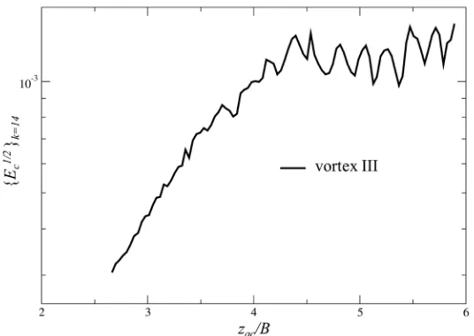
makes it unstable. The occurrence of the elliptic instability is suspected because of the short-wavelength disturbance, which is of the order of the core size. Furthermore, a spectral decomposition of the kinetic energy in the axial direction shows the exponential amplification of the energy contained by the Fourier mode k=14 which corresponds to the wavelength of the elliptical instability (see Figure 6). The instability saturates in vortex III resulting in a local transition to turbulence leaving behind a completely noncoherent vortex structure (see also Figure 5(a)).

At a downstream distance larger than z Bac ≈4.5 the dynamics of the

system is mainly governed by the behaviour of the two co-rotating vortices I and II. They rotate around each other and, due to the relatively small core ratios (

( ) ( )

a b < a b crit), the elliptical instability has time to develop. A clear sinusoidal

deformation of the vortex two vortex cores is observed in Figure 5(b), which is somewhat asymmetric resulting from the unequal core to spacing ratios of the individual vortices. The strong deformation of the vortex cores due to the instability leads to the exchange of vorticity between the two vortices and results in the unstable merger.

The occurrence of the elliptical instability is confirmed by a spectral analysis. The spectral decomposition in the axial direction shows the amplification of the energy contained by the most unstable mode corresponding to the elliptical wavelength, which is depicted for vortex I and II in Figure 7. After a transient regime one can clearly observe an exponential growth which indicates the linear regime of the elliptic instability. In this phase, the extracted growth rate (normalized by the turnover time of the vortex system) * ₄_π2 2

(

)

I II

b

σ

= ⋅

σ

Γ + Γ is approximately the same in the two vortices, i.e. σI ≈σII≈4.0, for the modes

corresponding to the most amplified wavelengths in each vortex (respectively

3.210 I aI

λ ≈ _and λII aII ≈3.952). An explicit formula was obtained by Le

[image:11.595.240.508.501.691.2]

Dizès et al.[23] through a theoretical analysis that predicts the temporal growth

Figure 6. Evolution of the most amplified Fourier mode (k=14) of the perturbation

(12)

[image:12.595.264.486.280.439.2]

aircraft wakes may be differ from those of Gaussian vortices.

Figure 7. Evolution of the most amplified Fourier mode (k=10) of the perturbation

energy contained in vortices I and II.

Figure 8. Comparison between simulation and theory [23] for vortex I and II in the

[image:12.595.262.489.488.665.2]

(13)

As a final remark, the development of the elliptic instability during the merging process modifies the final vortex structure. In particular, as shown in

Figure 9 and Figure 10, it causes the formation of a larger vortex core and leads to a decrease of the tangential velocity.

3.3. Three-Dimensional Results—Jet

[image:13.595.256.488.262.666.2]

In the previous Section, the formation and evolution of an aircraft wake was analyzed by focusing on the development of the intrinsic elliptic instability of the vortex system. In this Section, a different situation is considered where the vortex sheet interacts with an engine jet. The aim is first to find out whether and how the jet modifies the roll-up process of the vorticity sheet and, secondly, to analyze the mixing of an exhaust passive scalar in the wake.

Figure 9. Isocontours of u at a downstream distance of z Bac ≈7.65. Top panel: 2D

(14)

[image:14.595.248.504.65.298.2]

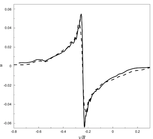
Figure 10. Velocity profiles through the center of the merged vortex at z Bac ≈7.65

(data extracted at locations indicated by the line in Figure 9): solid line, 2D simulation; dashed line, 3D simulation.

The computational domain is

(

L L L

x

, ,

y z

)

≈

(

1.0 ,1.6 ,0.072

B

)

and consists of

(

n n n

x

, ,

y z

)

=

(

395,601,36

)

gridpoints which are equally spaced in each of the

three directions. The first two dimensions are the same as the previous Section, while the axial length corresponds to the most unstable jet velocity profile in the simulations of Michalke and Hermann [31] (see also Ferreira Gago et al.[16], Paoli et al.[17] and Paoli et al. [18]). The jet axial velocity wj and the scalar

field Yj (representing any exhaust passive species) are initialized with a tanh

profile, F r

( )

=tanh 1 4 rj

θ

(

r r r rj− j

)

, where rj=0.072B is the jet radius,

2 2

r

=

x y

+

_{is the radial distance from the center and}θ =10rj is the

displacement thickness of the jet (see Paoli et al. [17] for details). With these profiles, one has

( )

1

(

) (

) ( )

2

j e a e a

w r = _ w w+ − w w F r− _₍₁₃₎

( )

1

(

) (

) ( )

2

j e a e a

Y r = _Y Y+ − Y Y F r− _₍₁₄₎

where subscripts a and e indicate, respectively, the free-stream conditions and the conditions at the center of the exhaust jet. In the present study, there is no co-flow, wa=0 and Ya =0 , while the exhaust velocity and scalar are,

respectively, we=0.18 and Ye=1.

(15)

[image:15.595.247.503.71.297.2]

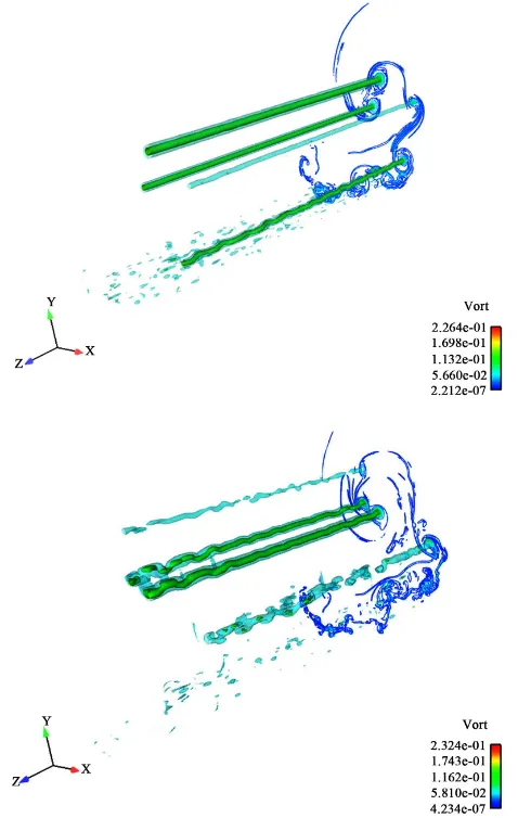
Figure 11. Isosurface of ω _{obtained by a three-dimensional computation of the}

jet/sheet system, at a downstream distance of z Bac ≈6.66.

magnitude at a late stage of the roll-up process, z Bac ≈6.96. First, the jet is

entrained around the multiple vortex system arising from the roll-up. Secondly, the jet continuously exchanges its axial momentum with the sheet by vortex stretching, causing the formation of complex three-dimensional vortical structures. Note that the figure displays the vorticity level 1.256

max e

ω ω

= ₍ω_max being the instantaneous maximum vorticity) which identifies the core of a axisymmetric Lamb-Oseen vortex. Indeed, the core of the merged vortex is clearly visible as well as the fine-scale eddies, remnants of the initial sheet vorticity and the jet turbulence, which are still wrapping around the core. This was already observed in previous simulations of jet/vortex interactions [16] [17], although in those cases, only a few azimuthal vortical structures (vortex rings) were formed around the core and only came from jet-generated turbulence. In the present case, the wake dynamics is more complex because the jet interacts with a vorticity sheet rather than a single well-formed vortex.

This strong momentum exchange and the turbulent diffusion induced by the jet affects the tangential velocity field of the final vortex. For example, the isocontour lines reported in Figure 12 shows the decrease of the (z-average) u-component of the velocity and the increase of the vortex core. The latter is due to the conservation of circulation Γ_{(not shown): as the peak azimuthal}

velocity decreases the core size must increase to keep Γ_{constant. The above}

picture is confirmed by the u-profiles in Figure 13, taken along the x const=

line marked in Figure 12, which shows that, at z Bac 7.65 the u-peak is

about half the value it had in the 2D case.

(16)

[image:16.595.267.479.65.439.2]

Figure 12. Isocontours of u at a downstream distance of z Bac ≈7.65. Top panel: 2D

simulations of the vortex sheet; bottom panel: 3D simulations of the jet/sheet system, averaged in the axial direction (the i-line through the core is also indicated).

Figure 13. Velocity profiles through the center of the merged vortex at z Bac ≈7.65

[image:16.595.277.473.498.676.2]

(17)

[image:17.595.258.491.73.460.2]

Figure 14. Isocontours of scalar field Yv at a downstream distance of z Bac ≈7.65:

top, 2D simulation of the vortex sheet; down, 3D simulations of the jet/sheet system, averaged in the axial direction (the initial location of the jet is also represented by thick lines).

that the combined effects of turbulent diffusion of the jet and its entrainment within the vortex sheet, enhances the dispersion of exhaust gases in the wake. This results in a larger plume area and causes a stronger dilution of the scalar field, which reaches a value of approximately 0.005, at a final stage of the merging process, compared to 0.476 in the the 2D laminar case.

4. Conclusions

(18)

Ressources en Informatique Scientifique) for providing the CPU hours. The authors also thank Airbus-Deutschland for providing the wind tunnel data.

References

[1] Spalart, P.R. (1998) Airplane Trailing Vortices. Annual Review of Fluid Mechanics, 30, 107-138. https://doi.org/10.1146/annurev.fluid.30.1.107

[2] Paoli, R. and Shariff, K. (2016) Contrail Modeling and Simulation. Annual Review of Fluid Mechanics, 48:393-427.

https://doi.org/10.1146/annurev-fluid-010814-013619

[3] Jacquin, L., Fabre, D., Geffroy, P. and Coustols, E. (2001) The Properties of a Transport Aircraft Wake in the Extended Near Field: An Experimental Study. 39th Aerospace Sciences Meeting and Exhibit, Reno, 8-11 January 2001, Number AIAA Paper 2001-1038.

[4] Crow, S.C. (1970) Stability Theory for a Pair of Trailing Vortices. AIAA Journal, 8, 2172-2179. https://doi.org/10.2514/3.6083

[5] Crouch, J.D. (1997) Instability and Transient Growth for Two Trailing-Vortex Pairs. Journal of Fluid Mechanics, 350, 311-330.

https://doi.org/10.1017/S0022112097007040

[6] Meunier, P. (2002) Etude expérimentale de deux tourbillons corotatifs. PhD Thesis, ONERA/Paris VI, France.

[7] Cerreteli, C. and Williamson, C.H.K. (2003) The Physical Mechanism for Vortex Merging. Journal of Fluid Mechanics, 475, 41-77.

https://doi.org/10.1017/S0022112002002847

[8] Meunier, P., Ehrenstein, U., Leweke, T. and Rossi, M. (2002) A Merging Criterion for Two-Dimensional Co-Rotating Vortices. Physics of Fluids, 14, 2757-2766.

https://doi.org/10.1063/1.1489683

[9] Leweke, T. and Williamson, C.H.K. (1998) Cooperative Elliptic Instability of a Vor-tex Pair. Journal of Fluid Mechanics, 360, 85-119.

https://doi.org/10.1017/S0022112097008331

[10] Meunier, P. and Leweke, T. (2001) Three-Dimensional Instability during Vortex Merging. Physics of Fluids, 13, 2747-2750. https://doi.org/10.1063/1.1399033

[11] Nybelen, L. and Paoli, R. (2009) Direct and Large-Eddy Simulations of Merging in Corotating Vortex System. AIAA Journal, 47, 157-167.

(19)

DOI: 10.4236/ojfd.2018.82012 179 Open Journal of Fluid Dynamics [12] Myake-Lye, R.C., Brown, R.C. and Kolb, C.E. (1993) Plume and Wake Dynamics,

Mixing and Chemistry behind a High Speed Civil Transport Aircraft. J. Aircraft, 30, 467-479. https://doi.org/10.2514/3.46368

[13] Jacquin, L. and Garnier, F. (1996) On the Dynamics of Engine Jets behind a Transport Aircraft. 78th Fluid Dynamics Panel Symposium, Number NATO-AGARD-CP-584.

[14] Gerz, T. and Ehret, T. (1996) Wingtip Vortices and Exhaust Jets during the Jet Re-gime of Aircraft Wakes. Aerospace Science and Technology, 1, 463-474.

https://doi.org/10.1016/S1270-9638(97)90008-0

[15] Brunet, S., Garnier, F. and Jacquin, L. (1999) Numerical/Experimental Simulation of Exhaust Jet Mixing in Wake Vortex. 37th Aerospace Sciences Meeting and Exhibit, Reno, 12-15 January 1999, Number AIAA 1999-3418.

[16] Ferreira Gago, C., Brunet, S. and Garnier, F. (2002) Numerical Investigation of Turbulent Mixing in a Jet/Wake Vortex Interaction. AIAA Journal, 40, 276-284.

https://doi.org/10.2514/3.15059

[17] Paoli, R., Laporte, F., Cuenot, B. and Poinsot, T. (2003) Dynamics and Mixing in Jet/Vortex Interactions. Physics of Fluids, 15, 1843-1850.

https://doi.org/10.1063/1.1575232

[18] Paoli, R., Nybelen, L., Picot, J. and Cariolle, D. (2013) Effects of Jet/Vortex Interac-tion on Contrail FormaInterac-tion in Supersaturated CondiInterac-tions. Physics of Fluids, 25, Ar-ticle ID: 053305. https://doi.org/10.1063/1.4807063

[19] Wang, F. and Zaman, K.B.M.Q. (2002) Aerodynamics of a Jet in the Vortex Wake of a Wing.Journal of Aircraft, 40, 401-407.

[20] Fares, E., Meinke, M. and Schroeder, W. (2000) Numerical Simulation of the Inte-raction of Wingtip Vortices and Engine Jets in the near Field. 38th Aerospace Sciences Meeting and Exhibit, Reno, 10-13 January 2000, Number AIAA 2000-2222. [21] Métais, O. and Lesieur, M. (1992) Spectral Large-Eddy Simulation of Isotropic and

Stably Stratified Turbulence. Journal of Fluid Mechanics, 239, 157-194.

https://doi.org/10.1017/S0022112092004361

[22] Ducros, F., Comte, P. and Lesieur, M. (1996) Large-Eddy Simulation of Transition to Turbulence in a Boundary Layer Spatially Developing over a Flat Plate. Journal of Fluid Mechanics, 326, 1-36. https://doi.org/10.1017/S0022112096008221

[23] Le Dizès, S. and Laporte, F. (2002) Theoretical Predictions for the Elliptic Instability in a Two-Vortex Flow. Journal of Fluid Mechanics, 471, 169-201.

https://doi.org/10.1017/S0022112002002185

[24] Stoessel, A. (1995) An Efficient Tool for the Study of 3D Turbulent Combustion Phenomena on MPP Computers. International Conference and Exhibition, Milan, 3-5 May 1995, 306-311. https://doi.org/10.1007/BFb0046645

[25] Gamet, L., Ducros, F., Nicoud, F. and Poinsot, T. (1999) Compact Finite Difference Schemes on Non-Uniform Meshes. Application to Direct Numerical Simulations of Compressible Flows. International Journal for Numerical Methods in Fluids, 39, 159-191.

https://doi.org/10.1002/(SICI)1097-0363(19990130)29:2<159::AID-FLD781>3.0.CO; 2-9

[26] Lele, S.K. (1992) Compact Finite Difference Scheme with Spectral-Like Resolution.

Journal of Computational Physics, 103, 16-42.

https://doi.org/10.1016/0021-9991(92)90324-R

(20)