Comparative Study of Optimized Wireless Sensor
Network Routing Protocols
Ahmed O. Eid
Zagazig University
Department of Computer and Systems Engineering
Zagazig University
Ibrahim E. Ziedan
Zagazig University
Department of Computer and Systems
Engineering
Zagazig University
ABSTRACT
Nowadays, Wireless sensor network applications are very important in most industrial fields. Most strategies are used to save energy of WSNs to prolong their life time. This problem attracted attention of many researches and many methods were proposed to optimize the energy consumption of WSNs. This paper presents a comparative study between two meta-heuristics algorithms are used to optimize this problem. One of them is the improved harmony search algorithm, and the other is the particle swarm optimization algorithm. Showing the strategies which are used to build its routing protocol and overviews on optimization algorithm which depend on build its solutions. Energy model used to calculate fitness of each solution. Improved algorithms are used in routing to solve the proposed problem. And propose termination criteria, simulation and results for each algorithm. At last this of them preferred to implement.
Keywords
Wireless Sensor Network, Routing Protocols, meta-heuristic, Harmony Search, particle swarm
1.
INTRODUCTION
In the last period , due to widely use of wireless sensor networks in different applications as military surveillance[1], environment monitoring[2], infrastructure protection[3] etc. WSN is considered as one of the most important technologies receiving tremendous attention from both academia and industry all over the world. Wireless sensor nodes are positioned by localization algorithm with GPS system[4]. WSN can be used in small scaled applications which is composed of some hundreds of nodes which is called SWSN or large scaled applications which may be composed of some hundreds of SWSN[5]. Sensor nodes are powered by batteries so the life time of each node is limited. The process of regeneration of power for nodes is an impossible process in large scale application. At the same time, energy saving in nodes is very important to ensure service continuity[5],[6]. Energy is consumed in sending data from source nodes to sink nodes. Data must consume small amount of energy and preferred to occur in small time. Many researches discussed this problem with different methods. One of the methods for saving energy is duty cycle secluding. Duty cycle can be classified into sleep secluding and route selection[7]. The operation of the node to sleep or wake up is called sleep secluding. Sleep secluding is designed for multi-hop WSN there is a great achievement of saving energy[7]. In sleep secluding the node can wake up and prepare a packet and send it at any time but only receive at the period of wake up only. Sleep secluding can be synchronous or asynchronous [8]. Synchronous sleep secluding neighbor nodes aggregated for sleeping pattern (if neighbor nodes wanted to change their active/sleep states, the states are changed concurrently)[8]. So the design of routing protocols for this type is very simple.
But in asynchronous sleep secluding, each node determines its active/sleep state independently. So the nodes are different in phase of secluding. Route selection has two main tasks. One of them is the collection of the routing information and the other is the forward path decision. Routing information can be classified into global routing information and local routing information. Global routing information includes network topology used in routing; nodes sleep secluding and end-to-end distance from a sensor node to a sink node. This global information can be obtained from control message from sink node. But local information includes one or two neighbor distance and one or two neighbor sleeping secluding [9], [10]. Meta heuristic algorithms are used also to find solutions for saving energy for WSN as harmony search algorithm [11], ant colony algorithm [12] and piratical swarm algorithm [13]. Meta heuristic is used when a path of solution is not required but the final solution only is important. Meta heuristic algorithms are used to send data from source to destination with small energy consumption.
Related works
M. Hasnat, M. Akbar, Z. Iqbal, Z. Khan, U. Qasim, and N. Javaid presented a B-DEEC protocol (Distributed energy efficient clustering protocol) for WSNs. It depends on a meta-heuristic algorithm called artificial bee colony (ABC). This protocol operation increases the life time of WSNs and increase its reliability. ABC algorithm derives its operation from honey bees in the way of foraging. It optimizes the next node selection so it decreases energy consumption of sending data and increases the life time of WSNs[14].
C. Sivakumar, and P. L. Parthiban presented IACO algorithm (improved ant colony algorithm). It uses fractional Brownian motions to improve the search way to improve the exploration capability. It maintains a good balance between exploitation and exploration abilities and improves energy efficiency of WSNs by selecting the optimal next node for sending data from source to destination[12].
D. Lobiyal, C. Katti, and A. Giri presented VANET (vehicular ad-hoc network) routing performance problem. Because of the large combinations of the values of parameters used in it, it is difficult to find optimal combinations. Algorithms depending on particle swarm have been proposed to find optimal combination of VANET[15].
2.
NETWORK MODEL FOR APPLYING
EACH ALGORITHM
routing algorithm. Each node has a unique ID. All nodes have the ability of computing its remaining power and communicating with each other by CSMA-CA protocol[4]. At the beginning of initiation of network the routing protocols steps are as follow
Step1: Sink node broadcasts a packet containing a number of hops initialized to zero to sensor nodes, when sensor nodes in the communicating range of sink node receive this packet, a minimum number of hops to sink node has been registered and neglect packet containing higher number. Then it sets number of hops plus one to the packet and sends it to its neighbor’s nodes. By this way each node has the minimum number of hops to the sink node.
Step2: Each node sets a packet containing its residual energy, number of hops to the sink node and IDs of its neighbor nodes then sends it to the sink node by single hop.
Step3: Sink node executes the routing algorithm and find best path from each node and send packet containing best forward path for each node in single hop.
Step4: When a source node senses a new data it set it in a packet and adds its residual energy to this packet and sends it to next node in forward path that is registered in its memory.
Step5: When a next node receives a packet it adds its residual energy, removes nodes that have been visited from the forward path, sends it to the next hop node and continues with this step until the packet reaches the sink node.
Step6: When a sink node receives a packet it processes the sent data and sends it to the specialists, executes the routing algorithm, calculates the new best forward paths for the nodes in the forward path and sends them to nodes in single hops.
2.2
Particle swarm optimization algorithm
A wireless sensor network is divided into two sections one of them is sensor nodes and the other is gateway nodes. Sensor nodes are used to sense useful data and send it to one of the gateway nodes. A sensor node could communicate with any gateway node but a gateway node must be in communicating range of a sensor node. Gateway nodes communicate with each other to reach sensed data by sensor node to specialist. Sensor nodes communicate with gateway node with TDMA[4], gateway nodes communicating with specialist by CSMA/CA[4]. There is more than one gateway node in the communicating range of sensor node but each sensor node can deal with one of them. Sensor nodes collect local sensed data and divided the data into rounds each node send its round to corresponding gateway node. Gateway node aggregates the local data and neglects the random of it then sends it to a specialist.Step1: the beginning each node from sensor nodes and gateway nodes has a unique ID each node broad cast it’s ID using CSMA/CA protocol.
Step2: The gateway node collects IDs from the sensor node and the other gateway nodes in communicating range of it and sends them to the base station.
Step3: The base station executes the routing algorithm and clustering algorithm. The execution of routing algorithm is first, and then information from it is used in clustering.
Step4: Each gateway node is informed by the next hop to the base station and each source node is informed by the gateway that will deal with it.
3.
NETWORK MODEL FOR APPLYING
EACH
3.1
Improved harmony search algorithm
Power consumption in WSN is estimated and the length of path are considered to describe the objective function[16]. Simple radio model of the circuit of transmitting or receiving dissipates E_elec=50 nj⁄bit for one bit and transmitted amplifier E_amp=0.1 nj⁄(bit⁄m^2 ) for one bit in one meter, to transmit k bits message in d meters power consumption of sending (1) and receiving (2) areETX k, d = Eelec ∗ k + Eamp ∗ k ∗ d2 (1)
ERX = Eelec ∗ k
(2)
So the power dissipated for path X={s,x1,x2,………,d} containing L nodes, energy consumption for transmitting a k-bits message along this path (3) is
𝐄 𝐱 = 𝐄
𝐓𝐗+ 𝐄
𝐑𝐗= 2 ∗ Eelec ∗ d − 1 ∗ k + Eamp ∗ k ∗ L−1i=1di,i+12 (3)
An objective function is selected to balance the energy consumption in the network and restrict the length of path (4) as possible[17]
𝐟(𝐱) =
𝐄 𝐱 ∗𝐥𝐄𝐦𝐢𝐧∗𝐄𝐚𝐯𝐠
(4)
Where the minimum residual energy of the node is E_min and E_avg is the average residual energy of all nodes in the path.
3.2
Improved harmony search algorithm
If the distance between transmitter and receiver is less than a threshold value d0 , the free space (fs) model is used, otherwise the multipath model (mp) is used[18].Energy required transmitting l bits message over distance d is as follows
ET l, d =
lEelec + lεfsd2 for d < d0 lEelec + lεmpd4 for d > d0
Where Eelec is the energy required for electric circuit, εfs energy required for amplifier in free space and εmp energy required for amplifier in multiple path.
Energy required for receiving data l-bit message at any node
ER(i) = lEelec
Digital coding, modulation, filtering and spreading of the signal effect on Eelec and the distance between transmitter and receiver effect on εmp and εfs .
Objective function is to maximize the life time of the WSN, PSO achieve this propose by maximize life Time of channel and minimize the Average distance between sensor nodes and their corresponding gateway.
Ecluster gi = ni× ER+ ni× EDA× ET(gi, nexthop gi )
Where EDA is the aggregation energy consumption, gi is the gateway and ni is the number of sensor nodes.
Eforward gi = NIN gi × ER+ NIN gi
× ET(gi, nexthop gi )
l(i) = EResidual gi
EGateway gi
Where l(i) is the life Time of WSN.
Fitness α l
As maximize the life time of average distance the maximum fitness is obtained. To minimize the average distance:
AvegDist =1
N dist(si N
i=1
, CHi)
Fitness α 1 AvegDist
4.
PROPOSED ALGORITHMS
4.1
Improved harmony search algorithm
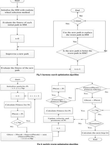
The harmony Search algorithm steps to achieve optimization of wireless sensor network of sending data from sensor node to sink node as shown in Fig 3.4.2
Particle swarm optimization algorithm
The Particle swarm algorithm steps to achieve optimization of wireless sensor network of sending data from sensor node to sink node as shown in Fig 4.5.
SIMULATION AND RESULTS
5.1
Improved harmony search algorithm
These results were developed by C++ programming language on a PC with 2.3 GHZ, Intel core I7, 7610 QM processor and 8 GH ram to analyze the energy of sensor node and life time.Metrics used to measure the performance of algorithm are:-
Average residual energy, the standard deviation of residual energy related to the average energy of all nodes and the standard deviation of residual energy level of all node respectively.
The minimum residual energy and the network life time denoted by the residual energy of the node with lowest residual energy among all nodes and the number of rounds that the network have sustained until any node runs out of energy.
[image:3.595.311.548.71.217.2]The energy level of all nodes is set to 10 J, and all nodes send packets to sink node periodically. Simulation parameters are as following:-
Table 1. Simulation parameters
Parameter Value
Packet size 4098 bits
Communication radius 150 m
HMS 5
HMCR in IHSBEER HMCRmin = 0.2
, HMCRmax = 0.9
HMCR in HSBEER HMCR=0.7 , PAR=0.02
Evolution items 500
α,β α=1,β=5
ρ 0.0
Initial pheromone 1.0
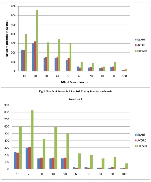
Simulation and results were obtained in two scenarios. First of them the energy is set to 10J for all nodes and each sensor node sends periodically packets to a sink node as Fig 1. The other scenarios three energy levels were used: 10J, 20J and 30J. These levels are uniformly distributed over the nodes. And each sensor node periodically sends packets to the sink node as Fig 2.
[image:3.595.309.548.363.653.2]5.2
Particle swarm optimization algorithm
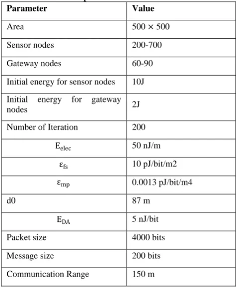
This simulation and results were performed with MATLAB R2012b and C-Programming Language. Simulation parameters are for the network as follows[18]:-Table 2. Simulation parameters
Parameter Value
Area 500 × 500
Sensor nodes 200-700
Gateway nodes 60-90
Initial energy for sensor nodes 10J
Initial energy for gateway
nodes 2J
Number of Iteration 200
Eelec 50 nJ/m
εfs 10 pJ/bit/m2
εmp 0.0013 pJ/bit/m4
d0 87 m
EDA 5 nJ/bit
Packet size 4000 bits
Message size 200 bits
Fig 1: Result of Scenario # 1 at 10J Energy level for each node
Fig 2: Result of Scenario # 2 at 10 or 20 or 30 Energy level for each node
0
100
200
300
400
500
600
700
10
20
30
40
50
60
70
80
90
100
Networ
k
LI
fe
time
in
Roun
ds
NO. of Sensor Nodes
EEABR
ACORC
EEHSBR
0
100
200
300
400
500
600
700
800
900
10
20
30
40
50
60
70
80
90
100
Senrio # 2
EEABR
ACORC
Start
Initialize the HM with roulette wheel selection method
Evaluate the fitness of each initial path in HM
t=0
Improvise a new path
Evaluate the fitness of the new
path t=t+1
Is the new path is better the worst path in HM? Use the new path to replace
the worst path in HM t<tmax
Yes
End
No
Yes
No
Fig 3: harmony search optimization algorithm
Start
Initialize particles Pi Ɐi 1 ≤ i ≤ Np
i=1
Calculate Fitness for Ni
Pbesti = Pi
i ≤ Np
i = i + 1
Yes
Gbest = Pbestk | fitness(Pbestk) = min (fitness(Pbestk) ,
Ɐi 1 ≤ i ≤ Np No
i=1
Update velocity and positions of Pi Calculate Fitness for Pi
Fitness(pi) < Fitness( Pbesti)
Pbesti = Pi
Yes
Fitness(Pbesti) < Fitness( Gbesti)
No
Gbesti = Pbesti
i ≤ Np Yes
Yes
No
Terminate? No
No
Calculate the next hop Gi Yes
[image:5.595.54.519.78.689.2]End
PSO parameters for algorithm are as follows[19]:
Table 3. Simulation parameters
Parameter Value
Np 60
C1 1.4962
C2 1.4962
W 0.7968
VMax 0.5
VMin -0.5
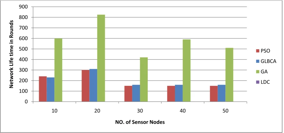
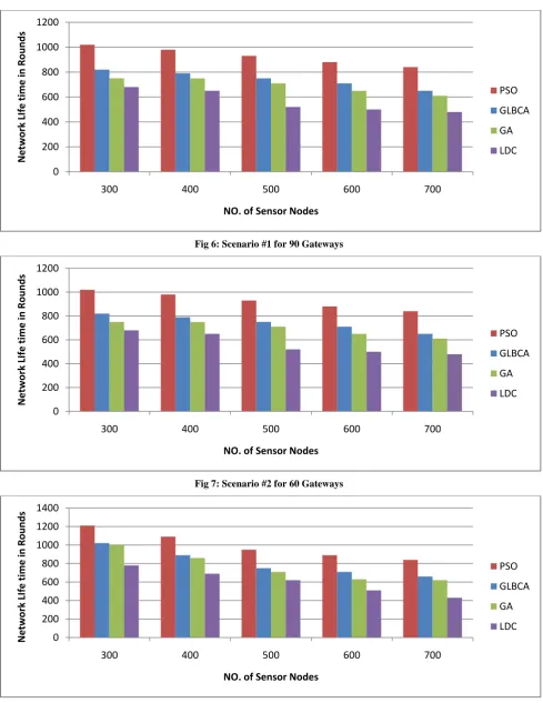
Simulation considers two different scenarios and the results of the proposed algorithm are compared with other algorithms as GA[20],GLBCA[21] and LDC[22]. The first one considers the base station to be positioned in aside of region with 60 nodes as in fig 5 and with 90 nodes as Fig 6 and the second consider base station to be at the center of the region with 60 nodes as in fig 7 and with 90 nodes as Fig 8.:
6.
TERMINATION CRITERIA
6.1
Harmony search optimization
algorithm
It uses tradition way to measure the life time of the network. At start the algorithm set for each node determine energy then send number of packets from each node then calculate the residual energy which each node have. Then determine the
life time of the network the network. If the residual energy of nodes is maximum, the longer life time of the network. If the residual energy of nodes is minimum, the shorter life time of the network.
6.2
Particle swarm optimization algorithm
Life time of the network can be defined by more than way[13]. The first way is the life time of the network until the first node die on the network. The second method is the life time of the network until the last node die (i.e. all nodes are died). The third method is until percent of nodes die (i.e. some of nodes are die)[13]. Some other consider the life Time of the network until the entire region are covered[23]. This algorithm considers the life time of the network until the first gateway node is died.7.
CONCLUSION AND FUTURE WORK
Results proved that particle swarm optimization algorithm is better than the harmony search algorithm. Number of nodes in particle swarm optimization algorithm network implementation is more than the harmony search algorithm network implementation. And the life time of network of particle swarm optimization is longer than the life time of the network of harmony search algorithm. In the future, Simulate other optimization algorithms such as sine- cosine algorithm and Ant colony algorithm in NS2 and compare results with these results. Implement these algorithms in real wireless sensor networks to see the effect of improving these algorithms.
Fig 5: Scenario #1 for 60 Gateways
0
100
200
300
400
500
600
700
800
900
10
20
30
40
50
Networ
k
LI
fe
time
in
Roun
ds
NO. of Sensor Nodes
PSO
GLBCA
GA
[image:6.595.55.546.416.647.2]Fig 6: Scenario #1 for 90 Gateways
Fig 7: Scenario #2 for 60 Gateways
Fig 8: Scenario #2 for 90 Gateways
0
200
400
600
800
1000
1200
300
400
500
600
700
Networ
k
LI
fe
time
in
Roun
ds
NO. of Sensor Nodes
PSO
GLBCA
GA
LDC
0
200
400
600
800
1000
1200
300
400
500
600
700
Networ
k
LI
fe
time
in
Roun
ds
NO. of Sensor Nodes
PSO
GLBCA
GA
LDC
0
200
400
600
800
1000
1200
1400
300
400
500
600
700
Networ
k
LI
fe
time
in
Roun
ds
NO. of Sensor Nodes
PSO
GLBCA
GA
8.
REFERENCES
[1] T. He, S. Krishnamurthy, L. Luo, T. Yan, L. Gu, R. Stoleru, G. Zhou, Q. Cao, P. Vicaire, and J. A. Stankovic, “VigilNet: An integrated sensor network system for energy-efficient surveillance,” ACM Transactions on Sensor Networks (TOSN), vol. 2, no. 1, pp. 1-38, 2006.
[2] R. Szewczyk, A. Mainwaring, J. Polastre, J. Anderson, and D. Culler, "An analysis of a large scale habitat monitoring application." pp. 214-226.
[3] S. Kim, S. Pakzad, D. Culler, J. Demmel, G. Fenves, S. Glaser, and M. Turon, "Wireless sensor networks for structural health monitoring." pp. 427-428.
[4] P. Baronti, P. Pillai, V. W. Chook, S. Chessa, A. Gotta, and Y. F. Hu, “Wireless sensor networks: A survey on the state of the art and the 802.15. 4 and ZigBee standards,” Computer communications, vol. 30, no. 7, pp. 1655-1695, 2007.
[5] A. Thakkar, and K. Kotecha, “A new Bollinger Band based energy efficient routing for clustered wireless sensor network,” Applied Soft Computing, vol. 32, pp. 144-153, 2015.
[6] Y. Zhu, and L. M. Ni, "Probabilistic approach to provisioning guaranteed qos for distributed event detection." pp. 592-600.
[7] J. Hao, B. Zhang, and H. T. Mouftah, “Routing protocols for duty cycled wireless sensor networks: A survey,” IEEE Communications Magazine, vol. 50, no. 12, 2012.
[8] G. Anastasi, M. Conti, M. Di Francesco, and A. Passarella, “Energy conservation in wireless sensor networks: A survey,” Ad hoc networks, vol. 7, no. 3, pp. 537-568, 2009.
[9] R. Beraldi, R. Baldoni, and R. Prakash, “A biased random walk routing protocol for wireless sensor networks: The lukewarm potato protocol,” IEEE Transactions on Mobile Computing, vol. 9, no. 11, pp. 1649-1661, 2010.
[10]K. P. Naveen, and A. Kumar, "Tunable locally-optimal geographical forwarding in wireless sensor networks with sleep-wake cycling nodes." pp. 1-9.
[11]B. Zeng, and Y. Dong, “An improved harmony search based energy-efficient routing algorithm for wireless sensor networks,” Applied Soft Computing, vol. 41, pp. 135-147, 2016.
[12]C. Sivakumar, and P. L. Parthiban, “Energy Efficient Traffic Protocol in Wireless Sensor Networks Using Improved Metaheuristic Algorithm.”
[13]P. Kuila, and P. K. Jana, “Energy efficient clustering and routing algorithms for wireless sensor networks: Particle swarm optimization approach,” Engineering Applications of Artificial Intelligence, vol. 33, pp. 127-140, 2014.
[14]M. Hasnat, M. Akbar, Z. Iqbal, Z. Khan, U. Qasim, and N. Javaid, "Bio inspired distributed energy efficient clustering for Wireless Sensor Networks." pp. 1-7.
[15]D. Lobiyal, C. Katti, and A. Giri, “Parameter value optimization of ad-hoc on demand multipath distance vector routing using particle swarm optimization,” Procedia Computer Science, vol. 46, pp. 151-158, 2015.
[16]D. Sahin, V. C. Gungor, T. Kocak, and G. Tuna, “Quality-of-service differentiation in single-path and multi-path routing for wireless sensor network-based smart grid applications,” Ad Hoc Networks, vol. 22, pp. 43-60, 2014.
[17]I. F. Akyildiz, and M. C. Vuran, Wireless sensor networks: John Wiley & Sons, 2010.
[18]W. B. Heinzelman, A. P. Chandrakasan, and H. Balakrishnan, “An application-specific protocol architecture for wireless microsensor networks,” IEEE Transactions on wireless communications, vol. 1, no. 4, pp. 660-670, 2002.
[19]D. Bratton, and J. Kennedy, "Defining a standard for particle swarm optimization." pp. 120-127.
[20]P. Kuila, S. K. Gupta, and P. K. Jana, “A novel evolutionary approach for load balanced clustering problem for wireless sensor networks,” Swarm and Evolutionary Computation, vol. 12, pp. 48-56, 2013.
[21]C. P. Low, C. Fang, J. M. Ng, and Y. H. Ang, “Efficient load-balanced clustering algorithms for wireless sensor networks,” Computer Communications, vol. 31, no. 4, pp. 750-759, 2008.
[22]A. Bari, A. Jaekel, and S. Bandyopadhyay, “Clustering strategies for improving the lifetime of two-tiered sensor networks,” Computer Communications, vol. 31, no. 14, pp. 3451-3459, 2008.