Effect of clay content and distribution on hydraulic and geophysical properties of 1
synthetic sand-clay mixtures 2
3 4 5 6
Gordon Osterman: Department of Earth and Environmental Science, Rutgers University-7
Newark, Newark, NJ, USA; gko4@rutgers.edu (corresponding author)
8
Madhuri Sugand: Lancaster Environment Centre, Lancaster University, Lancaster, UK, 9
Currently at the REACH Centre, Lancaster University, Lancaster, UK; 10
madhurisugand@outlook.com
11
Kristina Keating: Department of Earth and Environmental Science, Rutgers University-12
Newark, Newark, NJ, USA; kmkeat@newark.rutgers.edu
13
Andrew Binley: Lancaster Environment Centre, Lancaster University, Lancaster, UK; 14
a.binley@lancaster.ac.uk
15
Lee Slater: Department of Earth and Environmental Science, Rutgers University-Newark, 16
Newark, NJ, USA: lslater@newark.rutgers.edu
17
18
ABSTRACT 19
Geophysical methods show promise for detecting the spatial variability of subsurface 20
clay content and its effect on subsurface hydraulic properties. We present a laboratory study that 21
examines the influence of clay content and distribution on the relationships between hydraulic 22
conductivity, K, and the physical and geophysical properties of the media. Two geophysical 23
methods are investigated: spectral induced polarization (SIP) and nuclear magnetic resonance 24
clay was homogenously mixed or was present as large (~5 mm) clusters distributed through the 1
sample. K varies moderately well (normalized root-mean square error, NRMSE = 0.393) with the 2
pore-volume normalized surface area, Spor, a proxy measure of clay content, in the homogenous 3
samples and poorly (NRMSE = 0.507) when the clustered samples are included in the fit. SIP 4
parameters show moderately good to excellent fits with Spor for homogeneous samples 5
(NRMSE=0.0783 to 0.139) and moderately good to good fits for clustered samples 6
(NMRSE=0.140 to 0.336) and the coefficients describing the polarizability of the samples depend 7
on clay distribution. NMR parameters vary moderately well with Spor in the homogeneous 8
samples (NMRSE=0.341 to 0.412) and poorly (NRMSE=1.08 to 6.04) in the clustered samples. 9
SIP parameters vary moderately well with K (NRMSE=0.301 to 0.466), however, the relationship 10
between the SIP parameters and K is compromised by the non-negligible polarization of the clay 11
clusters. NMR parameters show good to excellent fits with K (NRMSE=0.0789 to 0.116). For 12
both SIP and NMR, fitting homogeneous and clustered samples together does not compromise 13
the fit quality. These results suggest that the geophysical measurements are better predictors of K 14
in heterogeneous porous media than bulk measures of pore geometry such as Spor. 15
INTRODUCTION 16
Accurate hydrogeological models require that the distribution of hydraulic properties in 17
the system is well-quantified. Typically, the hydrogeology is characterized using aquifer tests 18
performed in boreholes drilled into the groundwater system. In heterogeneous aquifers, a sparse 19
network of wells may not accurately resolve the spatial variation in hydraulic properties. Of 20
which are known to have a disproportionate impact on subsurface hydraulic properties, 1
particularly hydraulic conductivity (Neuzil, 1986; Keller et al., 1989). 2
Geophysical methods offer relatively fast and easy means of assessing spatial variations 3
in the physical and hydraulic properties of the subsurface (see e.g. Binley et al., 2015) and have 4
been used to map clay in the subsurface for decades (e.g. Palacky, 1987). Two relatively new 5
methods in groundwater geophysics, spectral induced polarization (SIP) and nuclear magnetic 6
resonance (NMR), are sensitive to the physical properties of porous media that control fluid flow 7
(Weller et al., 2010; Minagawa et al., 2008), allowing researchers to develop petrophysical 8
models using SIP and NMR parameters to estimate hydraulic conductivity (Börner et al., 1996; 9
Revil et al., 2015; Seevers, 1966; Dlubac et al., 2013; Osterman et al., 2016). Furthermore, 10
studies have shown that SIP and NMR signals are sensitive to variations in clay content (e.g. 11
Vinegar and Waxman, 1984; Okay et al., 2014; Costabel and Yaramanci, 2013). 12
Clay distribution is known to control electrical measurements in synthetic sediments. 13
Wildenschild et al. (2000) tested the effect of montmorillonite distribution on electrical 14
conductivity measurements, hydraulic conductivity, and the hydraulic radius estimated using the 15
approach of Revil and Cathles (1999). They found that surface conduction decreased when the 16
clay was clustered as opposed to homogeneously distributed. Sugand (2015) extended the 17
approach of Wildenschild et al. (2000) to study the impact of clay distribution on SIP 18
measurements and SIP-hydraulic conductivity models. They found that while the SIP 19
measurements were sensitive to the distribution of clay, the tested SIP-hydraulic conductivity 20
distribution. However, their work did not include direct measurements of the pore geometry of 1
their samples. 2
Previous studies have examined the effect clay heterogeneity on the NMR response of 3
water-saturated sediments. Anand et al., (2006) found that increasing the kaolinite or bentonite 4
content within homogeneous sand-clay mixtures resulted in a shift in the NMR relaxation time 5
distribution to shorter relaxation times. However, increasing the clay content when distributed as 6
a laminated surface within a sand matrix caused a second, short relaxation time peak to appear. 7
In clay-bearing natural soils, Stingaciu et al. (2009) found that NMR relaxation time distributions 8
compared well with pore size distributions measured from mercury injection and water retention 9
curves. However, the authors found that the surface area normalized by pore volume did not 10
correspond to the pore geometry detected by the NMR measurements. The effect of 11
heterogeneous pore size distributions on NMR in unconsolidated materials has been studied in 12
microporous silica beads (Hinedi et al. 1997) and in zeolites (Swanson et al., 2015). In both 13
cases, the bimodal pore size distributions were reflected in the NMR relaxation time 14
distributions. However, Hinedi et al. (1997) found that the surface area normalized by pore 15
volume was dominantly controlled by the microporosity whereas the NMR measurements were 16
more sensitive to the intergranular pores. While these previous studies have examined the effect 17
of clay heterogeneity on the NMR response, they did not explore how the clay distribution 18
impacted the link between the NMR parameters and the hydraulic properties of the sediments. 19
In this laboratory study, we extend the work of Wildenschild et al. (2000), Anand et al. 20
(2006), and Sugand (2015) by posing the following research question: what are the impacts of 21
between geophysical (SIP and NMR) parameters and the measured physical and hydraulic 1
parameters? We mix clean, silica sand with up to 10% of kaolinite clay by mass and distribute 2
the clay either homogeneously or as large (~5 mm in diameter), randomly dispersed clay 3
clusters. The clay clusters are proxies for the heterogeneous clay distributions in natural 4
sediments such as thin sand lenses; although they are imperfect reflections of natural sediments, 5
they provide a strong contrast to compare homogenous clay distributions against. The results 6
from this study represent a step towards understanding how the distribution of clay in 7
unconsolidated sediments impacts measured geophysical parameters and petrophysical models. 8
9
THEORY 10
Hydraulic conductivity
11
Hydraulic conductivity (K, units of m/s), is defined in Darcy’s Law as the proportionality 12
constant linking the rate of fluid flow to the hydraulic head gradient across a porous medium and 13
quantifies the ability of a porous medium to conduct fluid flow. For unconsolidated samples, K is 14
typically measured directly in the laboratory using one of two Darcy flow experiments: a 15
constant head or a falling head experiment (Domenico and Schwartz, 1990). Alternatively, K can 16
be estimated from characteristic physical properties of the porous medium; combining Darcy’s 17
Law with the Hagen-Poiseuille Law shows that K is proportional to the square of a characteristic 18
pore size (Bear, 1972). Johnson et al. (1987) rigorously defined this length scale as the 19
However, it is difficult to measure the hydraulic radius directly, especially in unconsolidated 1
sediments, so researchers have explored using proxy measures of hydraulic radius to estimate K. 2
An alternate pore geometry used for estimating hydraulic conductivity is the pore-volume 3
normalized surface area (Spor, units of 1/µm), which is often considered to be inversely 4
proportional to the hydraulic radius. Spor can be calculated from, 5
Spor=SSAρg
1-ϕ
ϕ , (1)
where SSA is the specific surface area (m2/g), ϕ is the porosity (-), and ρg is the matrix density
6
(g/m2). Clay has a much higher SSA than sand and in unconsolidated sand-clay mixtures with a
7
single type of sand and clay Spor is a rough proxy for the clay content with high Spor values 8
indicating high clay content. 9
Estimating K from Spor can be done using the Kozeny-Carman capillary bundle model of 10
the form (Carman, 1939), 11
K=KCϕSpor -2, (2)
where AKC is a fitting coefficient that accounts for the tortuosity of the pore space and varies 12
based on the soil texture (Chapuis and Aubertin, 2003). Ozgumus et al. (2014) compiled a set of 13
AKC values from numerous computational and experimental studies ranging between 4–14×10-5
14
m/µm2/s. Although the exponent in equation 2 is typically set to 2 (Carrier, 2003), other
15
researchers have suggested alternative values. For instance, Pape et al. (1987) suggest a value of 16
The dependence of K on Spor in equation 2 suggests that increasing the clay content of a 1
porous medium will reduce K. Chapuis and Aubertin (2003) cautioned that equation 2 only holds 2
for clayey sediments when they are fully saturated and non-compacted. Furthermore, Spor is a 3
bulk property of a porous medium and equation 2 implicitly assumes that Spor is homogeneous 4
throughout the volume of interest. In heterogeneous sediments, equation 2 may not be valid. 5
6
Spectral induced polarization
7
SIP, which evolved from the use of induced polarization in mineral exploration, is 8
employed for a wide range of near-surface geophysical problems, including hydraulic parameter 9
estimation. In this section we briefly review the theory of SIP; more thorough presentations can 10
be found in: Vinegar and Waxman (1984); Revil and Florsch (2010); Weller et al. (2010); 11
Kemna et al. (2012); Revil (2012, 2013); Revil et al. (2017); and Weller et al. (2015a). The SIP 12
measurement involves injecting a sinusoidal alternating electrical current into a porous medium 13
at low frequencies (mHz to kHz) and measuring the resulting phase-delayed sinusoidal voltage. 14
The measured complex electrical conductivity σ* (S/m) can be decomposed into real (σ’) and
15
quadrature (σ”) components, 16
σ*f=|σ|eiθf=σ'f+iσ''f, (3)
tanθ=σ
''f
σ'f,
(4)
where |σ| is the magnitude of the complex conductivity, θ is the phase angle (rad), f is the 17
The σ’ component quantifies electrolytic conduction resulting from the unrestricted 1
electromigration of ions through both the pore fluid and the electrical double layer (EDL) that 2
forms at the fluid-mineral interface (Sen et al., 1988; Revil and Cathles, 1999), 3
= 1
+ . (5)
F is Archie’s electrical formation factor (Archie, 1942; Vinegar and Waxman, 1984) which is 4
related to the tortuosity-normalized porosity, σf is the saturating fluid conductivity, and σs' is the
5
in-phase surface conductivity at the pore interface. While F and σs' are functions of the pore
6
geometry (Weller et al., 2013, Revil 2013), the parameters cannot be readily disentangled from 7
σf, which makes σ’ a non-ideal parameter for petrophysical relationships (Slater, 2007). The σ” 8
component represents restricted electromigration, which results in a reversible build-up of ions, 9
or polarization, throughout the pore space. In saturated geological media composed of insulating 10
grains, ionic polarization is thought to be caused by two dominant mechanisms in the 0.01-100 11
Hz range: EDL polarization (Leroy et al., 2008; Revil, 2012; Revil, 2013, Revil et al., 2017) and 12
membrane polarization (Marshall and Madden, 1959; Titov et al., 2002). Both mechanisms are 13
strongly dependent on grain and pore geometry (Revil and Florsch, 2010; Bücker and Hördt, 14
2013) and relatively insensitive to σf (Weller et al., 2011).
15
A single, characteristic value of σ” is often used to represent an entire SIP spectrum and 16
σ” at 1 Hz σ1''Hz is commonly chosen as it is a frequency readily measurable using laboratory, 17
borehole, and field SIP equipment. Weller et al. (2010) compiled SIP data on homogeneously 18
mixed sand and sand-clay sediments from Slater and Glaser (2003) and Slater et al. (2006), 19
which showed an approximately linear relationship between σ1''Hz and Spor. Revil et al. (2017)
extend on this relationship and developed a model of electrical conduction in soils where σ1''Hz is 1
approximated by Spor as, 2
σ1''Hz= Spor
F1-ϕ. (6)
Here Cs = 7.36×10⁻² mS um/m per Revil et al. (2013; 2017) (see derivation in Appendix A).
3
Similar to the specific polarizability from Weller et al. (2010), Cs is a function of ionic density 4
and mobility in the Stern Layer at the fluid-mineral interface and therefore a second-order 5
function of pore fluid chemistry (Weller et al., 2011). However, the specific polarizability as 6
defined by Weller et al. (2010) is a proportionality constant between Spor and σ” which, 7
according to equation 6, suggests that the specific polarizability implicitly contains information 8
on F and ϕ whereas Cs is independent of these parameters. Note that the units given for Cs 9
simplify to (nS) but are reported as (mS um/m) to reflect the units of the measurements used to 10
derive Cs. 11
Petrophysical information may be extracted from the entire SIP spectrum by modeling it 12
with a phenomenological relaxation time model such as a Debye-decomposition (Nordsiek and 13
Weller, 2008; Zisser et al., 2010). In the Debye-decomposition approach to modeling SIP spectra 14
of Nordsiek and Weller (2008), σ*f is given by a superposition of N Debye models, 15
σ*f=σ01-mj
1-1 1+i2πfτj
N
j=1
-1
, (7)
mj
N
j=1
=mt=
σ∞-σ0 σ∞ ,
where mj (unitless) and τj (s) are the chargeability and the SIP relaxation time parameters for the 1
jth relaxation term, mt is the total chargeability of the pore space (Sumner, 1976), σ
∞ is the
2
conductivity magnitude at the high frequency asymptote and σ0 is the conductivity magnitude at
3
zero frequency. mt defines the relative change in the magnitude of σ* over the frequency
4
spectrum. The normalized chargeability (mn, units of S/m) is calculated by scaling mt by σ0,
5
mn=mtσ0. (9)
Weller et al. (2010) found that mn varies linearly with Spor, and Revil et al. (2017) gave the 6
following expression, 7
mn=
Spor
F1-ϕ, (10)
where Cm is similar to Cs and the specific polarizability (Weller et al., 2010). From Revil et al. 8
(2013; 2017), Cm =5.96×10⁻¹ mS um/m (see Appendix A).
9
K can be estimated from SIP parameters based on power-law relationships, 10
=
(σ1''Hz). (11)
=
mn2
. (12)
Where As and Ap are fitting coefficients (mS2/m/s). Equations 11 and 12 are simplified versions
11
of the equations in Weller et al. (2015a), which were derived from 22 samples of unconsolidated 12
sediments. In the version of equation 11 given in Weller et al., (2015a) the exponent for σ1''Hz is –
13
2.27, the exponent for F is –1.12, and As =1.19×10⁻⁶
mS
2/m/s; in the version of equation 12given in Weller et al. (2015a) the exponent for mn is -2.21, the exponent for F is –1.07, and Am 1
=9.55×10⁻⁵
mS
2/m/s. Note that these values of As and Am were originally defined for permeability2
(k) models where permeability was measured in units of m2. For water-saturated media at 25°C,
3
K=V*k, where V=1.10×10⁷m*s and has been used to scale the coefficients in Weller et al.
4
(2015a) for use here. Although the models we use are not exactly the same as those from Weller 5
et al. (2015a), the exponents are sufficiently similar that we can compare our results to theirs. 6
7
Nuclear magnetic resonance
8
Geophysical applications of NMR focus on the detection of hydrogen protons in pore 9
fluids, primarily in water and hydrocarbons, to assess their quantity and mobility. A thorough 10
review of proton NMR for geophysical applications and hydraulic parameter estimation is 11
provided in: Timur (1969); Banavar and Schwartz (1987); Morriss et al. (1997); Kleinberg and 12
Horsfield (1990); Howard and Kenyon (1992); Kenyon et al. (1995); Kleinberg (1996); 13
Godefroy et al. (2001); and Behroozmand et al. (2015). The NMR experiment consists of tipping 14
the nuclear spins of the protons away from their equilibrium orientation with a static magnetic 15
field using a secondary oscillating magnetic field. After terminating the secondary magnetic 16
field, the protons relax back to their equilibrium orientation, a process that produces a 17
measurable signal, A(t) that can be modeled as a superposition of M exponential decays, 18
At=A0hje-t T⁄ 2j M
j=1
where A0 (arbitrary units) is the signal magnitude at time t=0; hj (-) and T2j (s) are the signal
1
fraction and transverse relaxation time of the jth portion of the signal, respectively. The A
0 is
2
proportional to the number of protons in the pore space tipped into the transverse plane and thus 3
gives the water content in the pore space. 4
The measured T2 relaxation times arise from three parallel relaxation mechanisms,
5
T2 -1
=T2B -1
+T2S -1
+T2D -1
, (14)
where T2B is the bulk relaxation time, which corresponds to relaxation occurring due to dipolar
6
spin-coupling between water molecules, T2S is the surface relaxation time, which corresponds to
7
relaxation occurring due to proton-electron spin coupling at paramagnetic mineral sites at the 8
fluid-mineral interface, and T2D is the diffusion relaxation time, which quantifies the apparent
9
relaxation that results from the dephasing of protons as they diffuse through pore-scale magnetic 10
field inhomogeneities. As T2B and T2D contain little information concerning the pore geometries
11
controlling fluid flow, it is desirable to minimize or eliminate their influence. T2B has a constant
12
value for water (~3 s) that is much slower than T2S and can be subtracted with little impact on T2
13
(e.g. Keating and Knight, 2007). The effect of T2D can be mitigated by using a
Carr-Purcell-14
Meiboom-Gill, or CPMG (Meiboom and Gill, 1958) pulse sequence to rephase the proton spins 15
with very short pulse intervals, or echo times (Kleinberg and Horsfield, 1990; Anand and 16
Hirasaki, 2008). 17
Brownstein and Tarr (1979) found that T2S is controlled by the distance a proton travels
18
before interacting with a pore wall, which is related to the size of the pore, as well as the density 19
and distribution of paramagnetic impurities at the surface quantified by the surface relaxivity, ρ2
(µm/s) (Kleinberg, 1996). If relaxation occurs in the fast diffusion regime then each pore is 1
characterized by a single relaxation time T2j and signal amplitude hj (Brownstein and Tarr, 1979;
2
Kleinberg and Horsfield, 1990). Assuming ρ2 does not vary to a large degree within the observed
3
geological media (Foley et al., 1996), the distribution of T2 relaxation times in equation 13 may
4
be interpreted as a proxy for the pore size distribution of a system (Kleinberg, 1996), although in 5
certain geological environments (e.g. formations containing iron(III)-bearing minerals) this 6
assumption may not be true (Keating and Knight, 2012). 7
In relatively homogeneous porous media, the entire system may be characterized by a 8
single, characteristic relaxation rate T2S -1
, where, 9
T2S -1
=ρ2Spor. (15)
The most commonly used characteristic value from the T2 distribution is the mean-log relaxation
10
time T2ml as it incorporates information from the entire T2 distribution. We refer to surface
11
relaxivities derived using T2ml as ρ2ml. The relaxation time at the peak of the distribution, T2p, has
12
also been shown to correlate well with the hydraulic radius (Keating, 2014; Osterman et al., 13
2016) and to be well suited for estimating K (Dlugosch et al., 2013). Here we refer to surface 14
relaxivities derived using T2p as ρ2p. Godefroy et al. (2001) found for a set of clean silicon
15
carbide samples that ρ2 ranged from 3≤ρ2≤5 µm/s. Similarly, Kleinberg (1996) found that ρ2=3
16
µm/s for quartz. Note that the derived value of ρ2 depends on the characteristic T2 value and how
17
the pore geometry is measured. For example, Stingaciu et al. (2009) found that Spor was not a 18
good pore geometry to use for estimating ρ2 in natural, clay-bearing soils, as it did not reflect the
19
In regularized inversions commonly used to extract the relaxation time distribution from 1
NMR data, the choice of regularization parameter can strongly impact the shape of the T2
2
distribution and the location of peaks. T2ml is relatively robust to variations in the regularization
3
parameter, which makes it an appealing relaxation time to use. By contrast, T2p may vary to a far
4
greater degree as a function of the regularization parameter and caution must be exercised when 5
interpreting T2p.
6
Based on equation 15, K models such as the Schlumberger-Doll Research equation 7
(SDR) have been derived for NMR measurements (Seevers, 1966; Banavar and Schwartz, 1987) 8
with the form, 9
K=Bml/pϕNMR n
T2 2
, (16)
where ϕNMR is porosity estimated from the NMR signal amplitude A0, Bml/p refers to the fitting
10
coefficient where the subscript corresponds to the characteristic relaxation time used (ml for T2ml,
11
or p for T2p), and n is an exponent used to describe the tortuosity of the pore space. In the NMR
12
literature n is typically set to 4 (Kenyon et al., 1995). Maurer and Knight (2016) found that for a 13
broad range of borehole measurements in unconsolidated sedimentary environments, Bml =0.80– 14
4.70 m/s3 when n=4. Another model that is commonly used to estimate K is the Timur-Coates
15
(TC); the TC model is an empirical model that uses an estimate of the irreducible water volume, 16
determined from the NMR relaxation time distribution, to predict K (Timur, 1969; Coates et al., 17
1991). Other researchers have developed models for K or k that are optimized for specific 18
geologic materials, such as unconsolidated coarse grain materials (Dlugosch et al., 2013), fine 19
grain sediments (Daigle and Dugan, 2009), and fine-grain clay rich mudstones (Daigle and 20
1
MATERIALS AND METHODS 2
To test the effect of clay content and distribution in synthetic sand-clay mixtures on the 3
relationships between the measured physical and hydraulic parameters and the geophysical 4
parameters, we prepared 21 synthetic mixtures with varying ratios of sand and clay and collected 5
Spor, K, SIP, and NMR data on each sample. All measurements were run in 9.3 cm tall by 2.3 cm 6
diameter cylindrical acrylic sample holders specially designed to support K, SIP and NMR 7
measurements without disturbing or repacking the samples (see Wallace, 2015). The sand-clay 8
mass ratios of 100-0, 99-1, 95-5, and 90-10 were used. For each clay concentration, three 9
replicate samples were mixed to test the repeatability of the packing and saturation procedure. 10
Sample preparation
11
Measurements were conducted on mixtures of Wedron silica sand (Wedron Silica Co.) 12
and kaolinite clay (Fisher Scientific). The Wedron sand is a medium, well sorted, round, clean 13
sand with a narrow grain size distribution centered at 300 µm and a specific surface area 14
SSA=0.0388±0.0001 m2/g. The kaolinite is a non-swelling, 1:1 phyllosilicate mineral with
15
SSA=11.552 ±0.0179 m2/g.
16
Homogeneous samples were packed by first drying the sand and clay, then mixing 17
according to the following ratios: 100%, 99%, 95%, and 90% sand, by mass. Figure 1 shows 18
examples of the homogeneous and clustered samples with 10% clay prior to packing. The mixed 19
sediments were dry-packed into the sample holders, with care taken to ensure no clay layers 20
forming it into ~5 mm diameter balls (Figure 1c) which were oven dried overnight, separate from 1
the sand. To create the clustered samples, dry sand and clay clusters were alternately added to the 2
sample holder to ensure the ratio of sand to clay was precisely known. The same sand-to-clay 3
ratios were used for the clustered samples as the homogeneous samples. Care was taken to 4
ensure that the clay clusters were not in contact with each other. 5
The following naming convention was used for all samples: The first letter refers to the 6
sample type (H indicates homogeneously mixed and C indicates clay clusters), the following 7
number indicates the percentage of clay (00, 01, 05, or 10), and the final letter indicates which 8
repeat the sample is (A, B or C). For example, sample H01B refers to the second repeat of the 9
homogeneous 1% clay samples. 10
[image:16.595.69.410.398.548.2]11
Figure 1: Examples of dry samples prior to packing, (a) 90% sand mixed homogeneously with 12
10% clay; (b) 90% sand mixed with 10% clay clustered in ~5 mm balls; (c) clay clusters shown 13
with a US quarter for scale. 14
All samples were vacuum saturated by pulling a strong vacuum on the dry samples before 15
flooding the sample holder with a degassed 10 mM sodium chloride brine (corresponding to a 16
fluid conductivity of 0.11±0.01 S/m at 25°C). Electrolyte species and concentration were chosen 17
conductivities were determined by repeatedly measuring the outflow conductivity and waiting 1
for the fluid conductivity to stabilize. Full saturation was confirmed by comparing the known 2
sample volume to the estimated sample volume calculated from the mass of the saturating fluid 3
and solid matrix, using densities of 1.00 g/m3, 2.65 g/m3, and 2.6 g/m3 for the saturating fluid,
4
sand, and kaolinite. 5
Measurement methodologies
6
A constant head approach was used to measure hydraulic conductivity (see Domenico 7
and Schwartz, 1990) and K was estimated from the average of four inflow-outflow head 8
differentials. A Micromeritics ASAP 2020 surface area analyzer was used to measure SSA using 9
the Brunauer, Emmitt, and Teller, or BET, method of gas adsorption porosimetry (Brunauer et 10
al., 1938). We used krypton as the adsorbate due to the very low surface area of the Wedron 11
sand. Measured SSA was converted to Spor using the porosity calculated from the mass difference 12
between saturated and dry columns normalized by the sample volume. Although BET 13
measurements can underestimate the surface area in clays with large inter-granular surface area 14
(see e.g. Weller et al., 2015b), kaolinite is a 1:1 clay with limited inter-granular surface area and 15
so BET is an acceptable method for measuring SSA for the samples used in this study. 16
Samples for BET analysis were prepared in two ways. Homogenous samples were dried 17
and subsampled from their columns and packed into the BET sample holders. Subsampling was 18
not an appropriate technique for the clustered samples, so we instead recreated clustered samples 19
SIP samples were run on an Ontash and Ermac PSIP instrument (Ntarlagiannis and 1
Slater, 2014) in the frequency range from 10 mHz to 1 kHz with 5 logarithmically spaced 2
measurements per decade. Each measurement was replicated three times to ensure repeatability. 3
The instrument was capable of resolving phase angles as low as 0.1 mrad. In one pure sand 4
sample and three clustered clay samples, we observed low polarization in the 0.1–10 Hz 5
frequency range that resulted in phase angles smaller than 0.1 mrad; measurements at these 6
frequencies were excluded from analysis. For ease of comparison with literature results, we use 7
σ1''Hz as the characteristic SIP polarization magnitude parameter. To calculate mn, we calculated 8
mt-distributions and σ0 using the Monte-Carlo Markov Chain approach of Keery et al. (2012)
9
where random walk simulations sample a probability distribution of possible solutions. 10
Electrical measurements were conducted with a range of saturating fluid conductivities in 11
order to accurately measure F (Vinegar and Waxman, 1984; Weller et al. 2013; Revil et al., 12
2015). All SIP parameters are calculated from measurements at low salinity, corresponding to σf 13
values of approximately 0.11 S/m. For the homogeneous clay samples, high-salinity 14
measurements were unavailable for the samples presented here. However, electrical 15
measurements were conducted over a range of salinities corresponding to σf values ranging from 16
approximately 0.11 S/m to 10 S/m on an alternate set of sand-clay mixtures packed using the 17
same methodology, materials, and sand-clay ratios. A comparison of the Spor, SIP and NMR data 18
between the data presented here and the alternate data set shows a high degree of repeatability. 19
For each sand-clay ratio, we assign an average value of F from the same sand-clay ratio from the 20
alternate data set. For the clustered clay samples, electrical measurements were made at two 21
All NMR data were collected using a 2.0 MHz Magritek Rock Core Analyzer. The 1
CPMG pulse sequence was used with echo times of 200, 400, 800, and 1600 µs, a total 2
measurement time of 10 s, and a recovery time of 10 s. Three cycles of 16 stacks were collected 3
at each echo time to assess measurement repeatability. Measurements from the samples were 4
compared using the 200 µs echo time data; longer echo times were used to assess the influence of 5
T2D. Data were inverted using a non-negative least squares algorithm with second-order
6
Tikhonov regularization, producing a log-spaced T2 distribution from 100 µs to 10 s (Whittall et
7
al., 1991). The inversion regularization parameter was selected using the approach of Costabel 8
and Yaramanci (2013) to produce the simplest model that minimizes the data misfit. Using this 9
approach, the same regularization parameter was selected for all samples, allowing us to ignore 10
the impact of regularization on T2p. T2B was determined from an average of measurements on
11
three samples of 10 mM sodium chloride brine and found to be 2.9 s. 12
Characteristic T2-relaxation times T2ml and T2p were used for the petrophysical analysis.
13
To calculate T2ml, we first eliminated any portion of the T2 distribution associated with standing
14
water in the columns, as signal associated with this water is insensitive to the hydraulic 15
properties of the sand-clay mixtures. The effect of bulk relaxation was removed by subtracting 16
T2B from T2ml and T2p. Following the procedure of Keating and Knight (2007), we fit a linear
17
regression between the square of the echo time and inverse relaxation time to demonstrate the 18
negligible impact of T2D at an echo time of 200 µs. To ensure that relaxation occurred within the
19
fast diffusion regime, we calculated ρ2 from equation 15 to assess whether the samples met the
20
fast diffusion criteria, ρ2R/D < 0.1, where R (µm) is the average distance a proton travels during
21
relaxation and D (µm2/s) is the self-diffusion coefficient of water (Brownstein and Tarr, 1979;
22
1
Fitting coefficients and statistics
2
The fitting coefficients (AKC for equation 2, Cs for equation 6, Cm for equation 10, As for 3
equation 11, Am for equation 12, ρ2 for equation 15, and Bml and Bp for equation 16) were
4
calculated as the mean-difference between log-transformed independent and dependent 5
parameters, 6
%&' = exp 1
N + logy,j-logyj
-N
j=1
, (17)
where coef refers to the fitting coefficient, N is the number of data points, y,j is the jth dependent 7
variable, and yj is the jth independent variable, which we set equal to the left-hand side of the 8
relevant petrophysical equation or K model. To measure the quality of the fit, we calculate the 9
normalized root mean square error (NRMSE) from, 10
NRMSE= 1
log10y,max-log10y,min/ 1
N +log10y,j- log10yj -2 N
j=1
, (18)
where y,max is the maximum predicted value and y,min is the minimum predicted value. Since the 11
NRMSE normalizes for both the number of samples as well as the data range, we can compare 12
values of NRMSEbetween datasets. To assess the quality of the fits determined using equation 13
17, we use the following criteria: NRMSE<0.1 correspond to excellent fits, 0.1<NRMSE<0.3, 14
correspond to good fits, 0.3<NRMSE<0.5 correspond to moderately good fits, while NRMSE>0.5 15
1
RESULTS 2
All values of K, Spor, ϕ, F, characteristic SIP parameters (σ1’’Hz and mn), and characteristic
3
NMR parameters used in this study are reported in Table 1. K varies from 4.98×10⁻⁶ m/s to
4
2.74×10⁻⁴ m/s in the homogeneous samples, but only from 1.52×10⁻⁴ m/s to 2.83×10⁻⁴ m/s in the
5
clustered samples. Spor varies from 0.14 1/µm to 6.26 1/µm in the homogeneous samples and 6
from 0.63 1/µm to 5.68 1/µm in the clustered samples. For all samples, ϕ varies from 0.36 to 0.40 7
with a mean of 0.38, and F varies from 4.10 to 6.26. No trend in ϕ or F is observed with 8
[image:21.595.71.543.510.736.2]increasing clay content which is likely a result of the low clay contents investigated. 9
Table 1: List of physical and geophysical parameters used for this study. Physical parameters 10
include the hydraulic conductivity (K), the gravimetric porosity (ϕ), the pore volume normalized 11
surface area (Spor), and the electrical formation factor (F). The geophysical parameters include 12
the SIP quadrature conductivity measured at 1 Hz (σ1''Hz, the SIP normalized chargeability (mn), 13
the NMR-estimated porosity (ϕNMR), the NMR mean-log transverse relaxation time (T2ml) and the
14
NMR transverse relaxation time at the peak of the distribution (T2p).
15 16 Clay % Sample Name K (m/s) ϕ (-) Spor
(1/µm)
SIP parameters NMR parameters
F
(-)
σ1'Hz
(mS/m)
σ1''Hz
(mS/m) mn (mS/m) ϕNMR (-) T2ml (s) T2p (s) H o m o g e n eo u s
0 H00A 2.74×10⁻⁴ 0.39 0.16
5.92
(a)
28.2 --(b) 0.028 0.37 0.584 0.604
0 H00B 2.60×10⁻⁴ 0.40 0.14
29.8 0.017 0.118 0.37 0.606 0.649
0 H00C 2.11×10⁻⁴ 0.37 0.18
29.3 0.004 0.058 0.38 0.498 0.562
1 H01A 1.74×10⁻⁴ 0.37 0.70
5.84
(a)
28.2 0.042 0.421 0.37 0.356 0.487
1 H01B 1.41×10⁻⁴ 0.39 0.61
28.7 0.027 0.343 0.38 0.322 0.422
1 H01C 1.83×10⁻⁴ 0.39 0.57
28.9 0.021 0.259 0.38 0.384 0.476
5 H05A 4.95×10⁻⁵ 0.36 3.03
4.24
(a)
26.5 0.074 0.947 0.39 0.191 0.316
5 H05B 3.68×10⁻⁵ 0.37 2.69
28.6 0.062 0.901 0.41 0.179 0.274
5 H05C 4.63×10⁻⁵ 0.37 3.03
25.5 0.079 1.139 0.40 0.199 0.340
10 H10A 7.71×10⁻⁶ 0.36 5.27
5.10
(a)
26.4 0.107 1.782 0.40 0.103 0.073
10 H10B 6.12×10⁻⁶ 0.38 5.39
24.8 0.124 2.293 0.41 0.102 0.062
10 H10C 4.98×10⁻⁶ 0.37 6.26
C
lu
st
er
ed
1 C01A 2.83×10⁻⁴ 0.38 0.63 4.62
28.3 0.009 0.056 0.37 0.566 0.649
1 C01B 2.56×10⁻⁴ 0.39 0.68 4.78
30.0 --(b) 0.030 0.38 0.614 0.698
1 C01C 2.17×10⁻⁴ 0.39 0.68 4.59 29.9 --(b) 0.059 0.39 0.592 0.649
5 C05A 2.06×10⁻⁴ 0.38 2.99 4.51
29.8 --(b) 0.320 0.37 0.426 0.649
5 C05B 2.12×10⁻⁴ 0.38 2.96 4.76
37.4 0.037 0.596 0.36 0.448 0.649
5 C05C 2.41×10⁻⁴ 0.39 2.83 4.54
28.9 0.015 0.257 0.39 0.458 0.649
10 C10A 2.21×10⁻⁴ 0.39 5.68 4.61
30.9 0.012 0.364 0.37 0.361 0.698
10 C10B 1.52×10⁻⁴ 0.39 5.30 4.27
29.8 0.062 0.441 0.38 0.332 0.604
10 C10C 1.80×10⁻⁴ 0.39 4.79 4.37
31.6 0.039 0.669 0.37 0.362 0.698
a Approximated F values from identically prepared samples with similar physical and geophysical properties. b Measured phase angle below instrument resolution limit (<0.1 mrad)
1
K vs Spor
[image:22.595.71.541.103.237.2]2
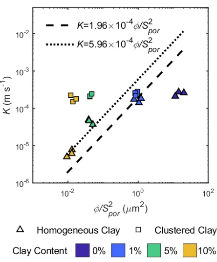
Figure 2 shows K plotted against ϕSpor-2 for all samples. For the data from the
3
homogeneous samples, the fits are moderately good (AKC = 1.96×10⁻⁴
m/µm
2/s and NRMSE =4
0.393, see Table 2). The misfit largely results from the 0% clay samples; removing the 0% clay 5
improves the fit (AKC = 4.46×10⁻⁴ m/µm2/s and NRMSE = 0.22). This shows that the
Kozeny-6
Carman model (equation 2) effectively models the homogenous sample data for samples with 7
≥1% clay by mass; however, at low clay contents (<1% by mass), the clay may still have a large 8
impact on the surface area but little to no impact on the hydraulic radius controlling K. When 9
considering the data from both the homogeneous and clustered samples, we find that the model 10
fits the data poorly (AKC = 5.96×10⁻⁴ m/µm2/s and NRMSE = 0.507, see Table 2) as the model is
11
not designed for highly heterogeneous samples. The values of AKC calculated for the 12
homogeneous samples and for all the samples are larger than the values given in Ozgumus et al. 13
(2014) of 4–14×10-5 m/µm2/s, which were compiled from a number of different studies. Thus, it
14
appears that the samples from this study have lower tortuosity than the samples analyzed in the 15
1
2
[image:23.595.184.406.193.461.2]3
Figure 2: K versus ϕ/Spor 2
for all samples. The dashed line and dotted lines show the fit of 4
Equation 2 to the homogeneous data and the entire dataset, respectively. The coefficients, (AKC), 5
and normalized root mean squared values are given in Table 2. 6
7
Table 2: Fitting coefficients and associated normalized root mean squared error (NRMSE) values 8
from for the Kozeny-Carman K model (equation 2) shown in Figure 2. The coefficients for the 9
models are given for fits to the data from the homogeneous samples and for the fits to the data 10
from all samples. Units for the literature values were converted to the units of the fitting 11
coefficients. 12
Coefficients Homogeneous Clay
Samples All Samples
Literature
Value NRMSE Value NRMSE
AKC 1.96×10⁻⁴ 0.393 5.96×10⁻⁴ 0.507 4–14×10-5 (a) m/µm2/s 2 1
a Ozgumus et al. (2014); range of coefficients were compiled from sources cited within.
1
Geophysical Results
2
Figure 3 shows SIP spectra for representative homogeneous and clustered samples over 3
the full range of clay content. Figures 3a and 3c shows σ’ and σ” spectra, respectively, for H00A, 4
H01A, H05A, and H10A, and Figures 3b and 3d shows σ’ and σ” spectra, respectively, for 5
H00A, C01A, C05A, and C10A. Overall, we do not observe any strong or consistent trends with 6
increasing clay content on σ’ for homogeneous or clustered clay samples and clay distribution 7
does not appear to have a strong impact on σ’ in the range of clay content tested. Increasing the 8
homogeneous clay content causes an increase in σ” over the entire frequency spectrum, 9
especially at frequencies above 100 Hz (Figure 3c), as expected from the literature (Okay et al., 10
2014). There is little increase in σ” with increasing clustered clay content (Figure 3d) in the 11
intermediate frequency range (0.1 to 10 Hz), contrasting with the behavior seen for the 12
homogeneous samples and suggesting that σ” is sensitive to clay distribution. At the low 13
frequency range, we observe an increase in σ” with increasing clay content that is robust across 14
1
Figure 3: SIP data collected for representative homogeneous and clustered samples for each clay 2
content (samples H00A, H01A, H05A, and H10A shown in (a) and (c); samples H00A C01A, 3
C05A, and C10A shown in (b) and (d)). SIP σ’ spectra for (a) homogeneous samples and (b) 4
clustered samples and SIP σ” spectra for (c) homogeneous samples and (d) clustered samples. 5
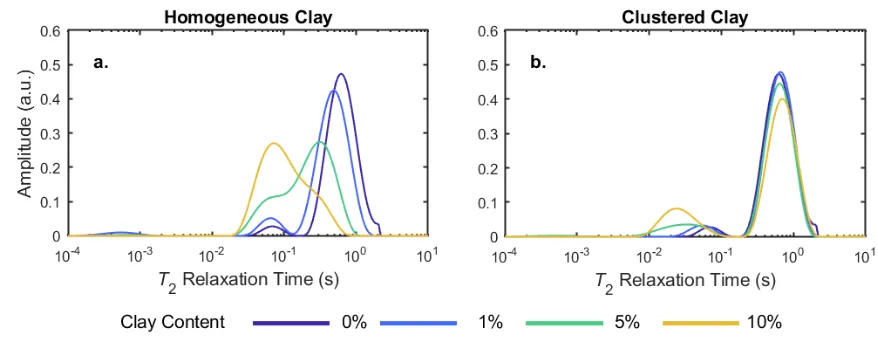
Figure 4 shows representative NMR T2 distributions for the homogeneous and clustered
6
samples over the entire range of clay content. Figure 4a shows T2 distributions for samples
7
H00A, H01A, H05A, and H10A, and Figure 4b shows T2 distributions for samples H00A, C01A,
8
C05A, and C10A. Increasing homogeneous clay content decreases the average pore size which 9
results in a shift in the dominantly mono-modal T2 distribution from long to shorter relaxation
10
times (Figure 4a). Similar results were shown by Anand et al. (2006) for homogeneous sand-11
[image:25.595.81.512.111.405.2]sand-illite. In the clustered samples, increasing clay content results in the growth of a second, 1
short-relaxation time peak and a small decrease in the amplitude of the original peak (Figure 4b). 2
In the bimodal distribution, the long T2 peaks correspond to the large, sand-bound pores, and the
3
short T2 peaks correspond to the small, clay-bound pores. These results match well with the T2
4
distributions from the bimodal sediments studied in Anand et al. (2006) and the natural soils 5
studied by Stingaciu et al. (2009). 6
We note that, for the pure sand samples, relaxation was not entirely in the fast diffusion 7
regime (0.09 ≤ κ ≤ 1.25) and so the second, short-relaxation time peak observed may represent a 8
second relaxation mode. This raises the possibility that some the signal in the shorter relaxation 9
times for the clustered samples may also represent faster relaxation modes in the pure-sand 10
portions of the sample in addition to the clay-bound water. For all other homogeneous samples, κ 11
< 0.1. 12
[image:26.595.75.514.460.635.2]13
Figure 4: NMR T2 distributions for representative (a) homogenous samples and (b) clustered
14
samples from each clay content (samples H00A, H01A, H05A, and H10A shown in (a); samples 15
1
Geophysical Parameters vs Spor
2
Figure 5 shows characteristic geophysical parameters plotted versus pore geometric 3
parameters (Spor/[F(1-ϕ)] in 5a and b, Spor in 5c and d). Here we compare the impact of clay 4
distribution on the relationship between the geophysical parameters and pore geometry by 5
calcuating fitting coefficients for the homogeneous and clustered sample data separately. All 6
coefficents and NRMSE values for each fit are given in Table 3. 7
For the relationship between Spor/[F(1-ϕ)] and σ1Hz'' (Figure 5a), we find a good fit for the
8
data from the homogeneous samples (Cs =1.02×10⁻¹ mS um/m and NRMSE=0.139) and a
9
moderate fit for the data from the clustered samples (Cs =2.15×10⁻² mS um/m and
10
NRMSE=0.336). When we examine the relationship between Spor/[F(1-ϕ)] and mn (Figure 5b), 11
we find there is an excellent fit for the data from the homogeneous samples (Cm =1.27 mS um/m 12
and NRMSE=0.0783) and a good fit for the data from the clustered samples (Cm = 0.259 mS 13
um/m and NRMSE=0.140). The fitting coefficients, Cs and Cm, for the data from the 14
homogeneous samples are up to two times higher than values calculated from the literature; in 15
contrast, the fitted coefficients for the clustered data are slightly lower than values given in the 16
literature (Cs =7.36×10⁻² and Cm =5.96×10⁻¹ mS um/m from Revil et al., 2013; and Revil et al.,
17
2017). This indicates that the values of the Cs and Cmpresented here represent endmember 18
values, where the high values correspond to homogeneous sand-clay media while the low values 19
Considering the relationship between Spor and 1/T2ml (Figure 5c), we find that there is a
1
moderately good fit for the data from the homogeneous samples (ρ2ml=3.57 m/s and
2
NRMSE=0.412) and a poor fit for the data from the clustered sample (ρ2ml=1.02 m/s and
3
NRMSE=1.08). Next when we consider the relationship between Spor and 1/T2p (Figure 5d), we
4
find there is a moderately good fit for the data from the homogeneous (ρ2p=3.20 m/s and
5
NRMSE=0.341), and a very poor fit for the data from the clustered samples (ρ2p=6.99×10⁻¹ m/s
6
and NRMSE=6.04). The values of ρ2ml and ρ2p for the data from the homogeneous samples are
7
within the range reported in the literature for clean quartz samples and clean silicon carbide 8
samples (ρ2=3–5 µm/s, Kleinberg, 1996; Godefroy et al. 2001). Although the literature values of
9
ρ2 were calculated using T2ml, we use them as an approximation of ρ2p.
10
1
Figure 5: Characteristic geophysical parameters plotted versus pore geometric parameters: SIP 2
parameters σ1Hz ''
(a) and mn (b) versus Spor/[F(1-ϕ)]; NMR parameters 1/T2ml (c) and 1/T2p (d)
3
versus Spor. The dashed line shows the line of best fit for the data from the homogeneous 4
equation 6, (b) equation 10, and (c-d) equation 15. The coefficients Cs (a), Cm (b), ρ2ml (c), and 1
ρ2p (d) were determined from fitting the log10 parameters in a least-squared sense and are given
2
along with the corresponding normalized root mean squared values in Table 3. 3
4
Table 3: Fitting coefficients and associated normalized root mean squared error (NRMSE) values 5
for the petrophysical models given in Figure 5. Coefficients from the data from the homogeneous 6
samples are given separately from the coefficients determined from the data from the clustered 7
samples; the fits are shown as dashed lines and dot-dashed lines in Figure 5, respectively. Note 8
that the units listed are taken directly from the fits, and that the literature values have all been 9
converted to these units where necessary. 10
Coefficient
Homogeneous Clay Samples
Clustered Clay
Samples Literature
Values
Value NRMSE Value NRMSE Units Equation Figure
Cs 1.02×10⁻¹ 0.139 2.15×10⁻² 0.336 7.36×10⁻² (a) mS um/m 6 5a
Cm 1.27 0.0783 2.59×10⁻¹ 0.140 5.96×10⁻¹ (a) mS um/m 10 5b
ρ2ml 3.57 0.412 1.02 1.08 3–5 (b) µm/s 15 5c
ρ2p 3.20 0.341 6.99×10⁻¹ 6.04 3–5 (b) µm/s 15 5d
a Values derived from coefficients given in Revil et al. (2013) and Revil et al., (2017).
b Godefroy et al. (2001); Kleinberg (1996); values given for silicon carbide and, at the low end, quartz sand.
11
Geophysical Parameters vs K
12
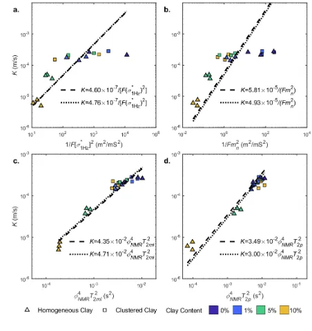
Figure 6 shows K plotted versus characteristic geophysical parameters. The plot of K 13
versus 1/ 1F σ1Hz'' 23 (Figure 6a) yields a moderately good fit for the data from the 14
homogeneous samples (As =4.60×10⁻⁷ mS2/m/s with NRMSE=0.301) as well as for the entire data
15
set (As =4.76×10⁻⁷
mS
2/m/s with NRMSE=0.301). We do not fit the clustered samples alone in16
Figure 6 alone as they do not demonstrate enough variation in K to extract meaningful statistics. 17
When we consider the relationship between K and 1/4F mn25 (Figure 6b) we observe moderately 18
good fits for the homogeneous sample data (Am =5.81×10⁻⁵ mS2/m/s with NRMSE=0.424) and for
the entire dataset (Am =4.93×10⁻⁵ mS2/m/s with NRMSE=0.466). We observe that both fitting
1
coefficients As and Am are remarkably consistent when fit to either the data from the 2
homogeneous samples or to data from both the homogeneous and clustered samples. All the 3
coefficients determined here are roughly half of the values from the literature (As =1.19×10⁻⁶
4
mS2/m/s and Am =9.55×10⁻⁵
mS
2/m/s, from Weller et al., 2010; Weller et al., 2015a). At high K5
(>10-4 m/s), we observe high variability in the SIP parameters but little variation in K; these
6
values correspond to measurements collected on the pure sand and the clustered clay samples, so 7
this observation likely occurs because the SIP measurements on these samples are nearing the 8
instrument resolution. At lower K values, the SIP parameters vary more closely with K; 9
recalculating fits for the homogeneous samples excluding the 0% clay samples yields good fits 10
(As =6.74×10⁻⁷ mS2/m/s with NRMSE=0.181, and Am =1.40×10⁻⁴ mS2/m/s with NRMSE=0.159)
11
with fitted coefficients that are closer to the literature coefficents. 12
When plotting K versus ϕNMR4 T2ml 2
(Figure 6c), we find there are excellent fits for the data 13
from the homogeneous samples (Bml =4.35×10⁻² m/s3 with NRMSE=0.0790) and for the
14
combined dataset (Bml =4.71×10⁻² m/s3 with NRMSE=0.0807). When we plot K versus ϕ NMR 4
T22p
15
(Figure 6d), we observe good fits for both the data from the homogeneous samples (Bp =3.49×10
-16
2 m/s3 and NRMSE=0.116) and for the combined dataset (Bp =3.00×10⁻² m/s3with
17
NRMSE=0.104). The good-to-excellent fits derived for both the NMR parameters when using the 18
entire dataset result from the clustered clay samples all grouping near the high-K limit of the 19
homogeneous samples. This grouping is expected from the T2-distributions (Figure 4) where
20
there is little variation in dominant mode of the T2 distribution as clay content increases. The
21
values of Bml and Bp determined here are substantially lower, by over an order of magnitude, than 22
the value found in the literature of Bml =0.8–4.70 m/s3 (Maurer and Knight, 2016). This
difference likely arises due to mineralogical differences between the silica-kaolinite samples 1
studied here and the aquifer material studied in Maurer and Knight (2016). 2
[image:32.595.63.515.182.661.2]3
Figure 6: Geophysical parameters plotted against K: SIP parameters 1/F 6σ1Hz'' 72 (a) and 1/F mn2
4
(b); NMR parameters ϕNMR4 T2 2ml (c) and ϕNMR 4
T22p (d). The dashed line and dotted lines show fitted
K-models for the homogeneous data and the entire dataset, respectively, given by (a) equation 1
11, (b) equation 12, and (c-d) equation 16. The coefficients ((a) As, (b) Am, (c) Bml and (d) Bp) and 2
normalized root mean squared values are given in Table 4. 3
Table 4: Fitting coefficients and associated normalized root mean squared error (NRMSE) values 4
from for the K models shown in Figure 6. The coefficients for the models are given for fits to the 5
data just for the homogeneous samples and for the fits to the data from all samples. The units for 6
all values were converted to be consistent with the units used in this study. 7
Coefficients
Homogeneous Clay
Samples All Samples Literature
Values Units Equation Figure
Value NRMSE Value NRMSE
As 4.60×10⁻⁷ 0.301 4.76×10⁻⁷ 0.301 1.19×10⁻⁶(a) mS2/m/s 11 6a
Am 5.81×10⁻⁵ 0.424 4.93×10⁻⁵ 0.466 9.55x10⁻⁵(a) mS2/m/s 12 6b
Bml 4.35×10⁻² 0.0790 4.71×10⁻²
0.0807 0.80-4.70 (b) m/s3 16 6c
Bp 3.49×10⁻² 0.116 3.00×10⁻²
0.104 0.80-4.70 (b) m/s3 16 6d
a Weller et al. (2015a); approximate value from their equation 27 and Figure 5b.
b Maurer and Knight (2016); average value given for borehole measurements in aquifer.
8
DISCUSSION 9
Our results demonstrate K is only well predicted from Spor, the proxy measure of clay 10
content, and ϕ for the homogenous samples. The clustered clay content had a minimal impact on 11
K over the range of clay contents, which results in a poor fit when equation 2 is used to model to 12
the entire dataset. This result is expected as fluid should primarily flow through the hydraulically 13
interconnected sand matrix between the clay clusters and Spor is not a good proxy for the inverse 14
hydraulic radius in the clustered samples. 15
The SIP data are sensitive to changes in Spor, as both σ1Hz'' and mn vary with Spor (Figures 16
5a and 5b) regardless of clay distribution. The linear correlation between the SIP parameters and 17
Florsch, 2010; Weller et al., 2010, Revil et al., 2017), but not in heterogeneous material, such as 1
the clustered samples reported here. The primary difference between the homogeneous and
2
clustered samples is that the coefficients Cs and Cm are higher for the homogeneous samples than
3
for the clustered samples, which supports the results of Wildenschild et al. (2000) who observed
4
higher DC surface conduction in their homogeneous clay mixtures compared to their clustered
5
clay samples. This makes sense as in-phase surface conductivity is known to be proportional to
6
the quadrature conductivity (Börner et al., 1996; Weller et al. 2013). Sugand (2015) also
7
observed higher quadrature conductivity in their homogeneous samples compared to their
8
clustered samples. Based on equations 6 and 10, clustered samples and homogeneous samples
9
with similar clay content, mineralogy, fluid chemistry, and saturation should theoretically
10
produce similar σ” and mn values. The decrease in these parameters for the clustered samples
11
suggests there is a decrease in the electrical current density within the clay clusters. This
12
indicates that the surface area available for polarization must be considered, where this “active
13
surface area” is a function of the distribution of mineral grains in a porous medium.
14
In Figure 3d, we observe a clear and repeatable increase in signal amplitudes at 15
frequencies lower than 1 Hz as a function of clay content. If the SIP measurement observes the 16
clay clusters as very large, clay-coated grains experiencing EDL polarization, it is possible that a 17
very low frequency (<0.01 Hz) peak would be associated with the clay clusters. Within the 18
clusters, high clay content may lead to a reduction in the ionic mobility similar to what Weller et 19
al. (2016) described for clay-bearing sandstones. These observations suggest that the active 20
surfaces controlling the SIP spectra for the clustered clay samples may be isolated to the outer 21
In the case of the homogeneous samples, the SIP data vary closely with K, especially 1
when the 0% clay samples are removed. However, the SIP parameters for the clustered samples 2
vary independently of K (Figures 6a and 6b). The non-negligible polarization of the clay clusters 3
compromises the overall fit between the SIP parameters and K and suggests that the length scale 4
controlling the SIP parameters may be more closely related to Spor than to the hydraulic radius in 5
the sand-clay mixtures. Despite the polarization of the clay clusters, the SIP-K models (Figures 6
6a and 6b) still provide superior fits for both homogeneous and clustered clay sample data 7
compared to the fits from the Kozeny-Carman equation (Figure 2). This suggests that the SIP 8
active surface is a better proxy for the hydraulic radius than Spor in the tested samples. 9
Considering the NMR results, we find that the NMR relaxation times vary with Spor 10
(Figures 5c and 5d) for homogeneous samples but only give moderately good NRMSE values. At 11
high clay content (≥5%) it appears that relationship between T2ml and Spor for the homogeneous
12
samples may become linear, suggesting that Spor may be a better proxy for inverse pore size at 13
higher clay content. However, at low clay content (<5%), the relationship appears nonlinear. 14
This is likely because clay content variation at low clay contents (≤1%) will cause 15
disproportionately large changes in surface area compared to pore size. These results 16
demonstrate the potential pitfalls in applying T2ml in equation 15 even in homogeneous sand-clay
17
systems where Spor may not be an effective proxy for pore size. The relationship between T2p and
18
Spor in Figure 5d is non-linear, indicating that T2p is not an appropriate measure of Spor in the
19
tested range. 20
For the clustered samples, there is no linear relationship between the NMR parameters 21
and Spor. This follows from examining the bimodal T2 distributions in Figure 4b where the T2
peak, controlled by the sand-bound pores dominates the T2 distribution while Spor is primarily
1
sensitive to the clay-bound surface area. This agrees with the results from Hinedi et al. (1997) 2
who found that Spor in microporous silica beads was dominated by the microporosity that 3
corresponded only to their fastest relaxation times. Further, our results support the findings of 4
Stingaciu et al., (2009) who found that equation 15 could not be used to link the bimodal T2
5
distributions to a bulk property like Spor in natural soils. It may instead be possible to represent 6
the pore space more effectively using a weak-coupling relaxation model (Grunewald and Knight, 7
2009; Keating and Knight, 2012) to distinguish between Spor in sand-bound and clay-bound pore 8
space. Ultimately, the NMR results in Figures 5c and 5d highlight the disconnect between the 9
NMR T2 distributions, which are sensitive to pore size distributions, and the bulk surface area
10
measured by gas adsorption. 11
The distinct peaks in the clustered clay samples suggest there is little inter-pore coupling 12
between the sand-bound water and the clay-bound water. We attribute this to the large size of the 13
clay clusters, which reduce the probability that water molecules will diffuse through both clay-14
and sand-bound pores. This agrees with the findings of Grunewald and Knight (2009; 2011) who 15
found that coarse heterogeneous sediments experienced less pore-coupling than fine-grained 16
sediments. It is possible, however, that pore coupling would be observed in samples with smaller 17
clay clusters or natural clay aggregates. 18
The fits between the NMR relaxation times and K (Figures 6c and 6d) are very good, 19
consistently producing NRMSE values close to or less than 0.1 even when including the clustered 20
sample data. The close fits show that the NMR parameters are better proxies of the hydraulic 21
taken when applying this result broadly, as NMR is a measure of bulk properties and is 1
insensitive to anisotropy. Taking the laminated clay systems studied by Anand et al., (2006) as 2
an example, if the laminations were oriented orthogonal to the hydraulic gradient, the hydraulic 3
radius would be controlled by the clay-bound porosity rather than the sand-bound porosity. This 4
means the shorter T2 peak would likely correspond to K. Since the T2 distribution contains no
5
directional information, it is impossible to know which T2 peak contains the essential information
6
about the hydraulic radius controlling K without additional information about pore connectivity. 7
Thus, the non-uniqueness of the NMR response compromises its sensitivity to K in 8
heterogeneous systems to a greater extent than our results indicate. Using pulsed-field gradient 9
NMR methods to measure diffusional length scales (e.g. Latour et al., 1995) or combining the 10
NMR measurements with additional measurements sensitive to anisotropy (e.g. SIP) may help to 11
overcome this limitation. 12
The low variability in ϕ, ϕNMR, and F indicate that these parameters do not have a strong 13
impact on the K models. Excluding these parameters from the K models in equations 2, 11, 12, 14
and 16 results in similar fitting coefficients and NRMSE values. These results support the 15
findings of Weller et al. (2015a), who found that F could be excluded from SIP-K models in 16
unconsolidated materials, as well as the results of Maurer and Knight (2016), who showed that in 17
unconsolidated aquifers that the n exponent in the SDR equation could be set to 0, negating the 18
influence of ϕNMR. In unconsolidated systems with little pore space tortuosity, there appears to be 19
no need to include ϕ, ϕNMR, or F in K-prediction models. A homogeneous, sandy system with low 20
(<10%) clay content, such as the sand underlying the CFB Borden site in Canada (Sudicky and 21
We experimentally show that the sensitivity of SIP and NMR parameters to clay 1
distribution in a sand matrix impacts the relationships between the physical and hydraulic 2
parameters and the geophysical parameters. SIP parameters are linearly correlated to the clay 3
content, with the correlation coefficient dependent on the clay distribution. The NMR relaxation 4
time distributions are very sensitive to the distribution of pore sizes, resulting in very strong fits 5
with K. As a result of their sensitivity to clay distribution, all geophysical parameters analyzed 6
proved to be predictors of K rather than Spor, which is not sensitive to clay distribution. This 7
suggests that geophysical methods may provide accurate field-scale estimates of K in 8
heterogeneous geological environments where K models based on pore geometric parameters 9
may be limited. Further study is necessary to understand the sensitivity of field SIP and NMR 10
measurements to hydrogeological heterogeneity. This is particularly important for NMR 11
measurements, which are only sensitive to bulk subsurface properties. 12
Future work should also focus on testing higher clay concentrations where the clusters 13
may begin to impact K, different clay types expanding on the work of Anand et al. (2006) and 14
Sugand (2015), and realistic geological analogs. The NMR results for the clustered samples in 15
Figure 4b match closely with the laminated kaolinite samples from Anand et al. (2006), 16
suggesting that they can be used to simulate systems where clay lenses are oriented parallel to 17
the hydraulic gradient. However, further tests must be run to simulate a scenario where clay 18
lenses are oriented orthogonally to the hydraulic gradient. Wildenschild et al. (2000) and Sugand 19
(2015) have tested a small number of anisotropic sand-clay samples, observing that electrical 20
measurements are sensitive to clay-lens orientation. Further tests on anisotropic clay distributions 21