Numerical simulations of two dimensional and three dimensional shock wave/turbulent boundary layer interactions

Jian Fang1, Yufeng Yao2, Alexander A. Zheltovodov3 and Lipeng Lu1

1

National Key Laboratory of Science and Technology on Aero-Engine Aero-Thermodynamics, School of Energy and Power Engineering, Beihang University, Beijing, 100191, China

2

Faculty of Environment and Technology, Department of Engineering Design and Mathematics, University of the West of England, Bristol, BS16 1QY, United Kingdom

3

Khristianovich Institute of Theoretical and Applied Mechanics, Siberian Branch of Russian Academy of Science, Novosibirsk 630090, Russia

1. Introduction

The shock wave/turbulent boundary layer interaction (SWTBLI) happens ubiquitously in high-speed vehicles and their propulsion systems and has great influences on their performances. The researches of SWTBLI are persisted for more than 60 years, although, some flow mechanisms in it are still not completely understood and the prediction of it in engineering is far beyond satisfactory.1

The impinging shock-wave/flat-plate boundary layer interaction is a standard CFD case for two-dimensional (2D) SWTBLI, which represents the simplest SWTBLI configuration for the validation of turbulence models and computational methods. Although plenty of researches focused on this kind of flows2-5, the flow mechanism in it is still not well understood. Comparing with the 2D SWTBLI, the three-dimensional (3D) SWTBLI is even less studied and understood, although, it is closer to real flows and has special influences on the performances of intakes and control surfaces. Most researches of 3D SWTBLI are limited in the framework of experimental measurements6-12 and numerical simulations by solving Reynolds-averaged Navier–Stokes (RANS) equations13-16. The large-eddy simulation (LES) or direct numerical simulation (DNS), which can give detailed information of turbulent flows and greatly benefits the research of turbulence mechanisms, has not been applied in the 3D SWTBLI yet in published reports.17

With the help of the fast progress of high performance computing (HPC) technology and the recently developed numerical method, the present paper conducts the DNS of a Mach 2.25 impinging shock-wave/flat-plate boundary layer interaction and LES of a Mach 5 flow passing a single-fin with 23° deflection angle. The results are validated and flow property as well as turbulence mechanisms in 2D/3D SWTBLI are studied by analyzing the data.

2. Flow Configuration and Computational Setup

The governing equations in the present studied are taken as the compressible unsteady 3D Navier-Stokes (NS) equations in generalized curvilinear system. For the LES calculation, NS equations are filtered and the dynamic Smagorinsky model18,19 is used to calculate subgrid-scale eddy-viscosity model coefficients. The subgrid-scale heat flux is also calculated by the dynamics procedure.

a b

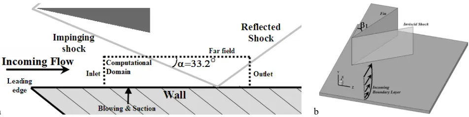
Fig. 1. Sketch maps of the flow configurations of (a): 2D SWTBLI and (b): 3D SWTBLI in the present study.

For the 2D SWTBLI case, the reference length is 1 inch, based on which the Reynolds number is 635000. A domain with the size of 7 × 1.2 × 0.2 is discretized by an orthogonal grid with 280 × 150 × 256 points. The grid’s points are concentrated towards the wall and the interaction position to enhance the resolution in these regions. The posteriori test showed the resolution reached the Kolmogorov length scale in both the undisturbed boundary layer (BL) and interaction region.

The reference length for the 3D SWTBLI is 1 mm, which make the Reynolds number is 3.7 × 107 _{. The size of the domain is (−20, 184.5) × (0, 35) × (0, 215) , which is}

about(−5.3𝛿₀, 18.6𝛿₀) × (0, 9.2𝛿₀) × (0, 56.6𝛿₀), in the scaling of the incoming boundary layer thickness 𝛿₀. Therefore, the computational domain is similar with that of the experimental measurement of Schülein7 and the RANS study of Salin et al.13. The grid has 1060×240×1420 points in the streamwise, normal to the bottom wall and spanwise directions respectively and it is smoothly stretched to ensure the resolution at the wall is below 1 viscous scale. It can be seen that, lots of grid points are spent in the spanwise direction due to the 3D property of the flow configuration.

The Euler terms of the NS equations are solved by using the newly developed seventh-order low-dissipation monotonicity-preserving (MP7-LD) scheme20, which is optimized from the original monotonicity-preserving (MP) scheme of Suresh and Huynh21 by reducing both the linear dissipation and nonlinear error. The diffusion terms are solved by using the sixth-order compact central scheme22. After all the spatial terms are solved, the residual terms are integrated in time by using the explicit three-step third-order TVD Runge-Kutta scheme23.

For both cases, the isothermal no-slip boundary condition (BC) is used at walls. The perfectly non-reflective BC is used at the outlet plane and the far-field surface, near which sponge layers are incorporated to reduce the reflection of numerical errors from boundaries. For the 2D case, the periodical BC is used at the lateral surfaces, while the free-slip BC is applied at the lateral surfaces of the 3D case, due to the non-homogeneous direction in the spanwise. The supersonic inflow condition is used at the inlet planes for both the cases, but the inflow turbulence is generated in different ways. For the 2D case, a laminar boundary profile is assigned at the inlet plane and the wall blowing and suction24,25 is used to trigger the boundary layer transition. A long transitional region is used to let the boundary layer fully developed, as shown in Fig. 2. For the 3D case, in avoid of using a long transitional zone, a time series of fully developed boundary layer slices from another independent LES is introduced to the inlet plane of the main LES.

The BL parameters at x=9.5 for 2D case and at inflow plane of the 3D case are given in Table 1. For the 3D case, the agreement of the BL parameters with the experiment is good

Table 1 Incoming Boundary Layer Parameter

𝑀0 𝑅𝑒0 𝛿,𝑚𝑚 𝛿∗,𝑚𝑚 𝜃,𝑚𝑚 𝑅𝑒𝛿 𝑅𝑒𝛿∗ 𝑅𝑒𝜃

2D Case 2.25 6.3×105/in 1.53 0.39 0.12 41100 11500 3100 3D Case 5.0 37×106/m 3.85 1.60 0.17 141000 58500 6900 Experiment7 5.0 37×106/m 3.8 1.6 0.16 - - -

3. Results and Discussions 3.1. 2D SWTBLI

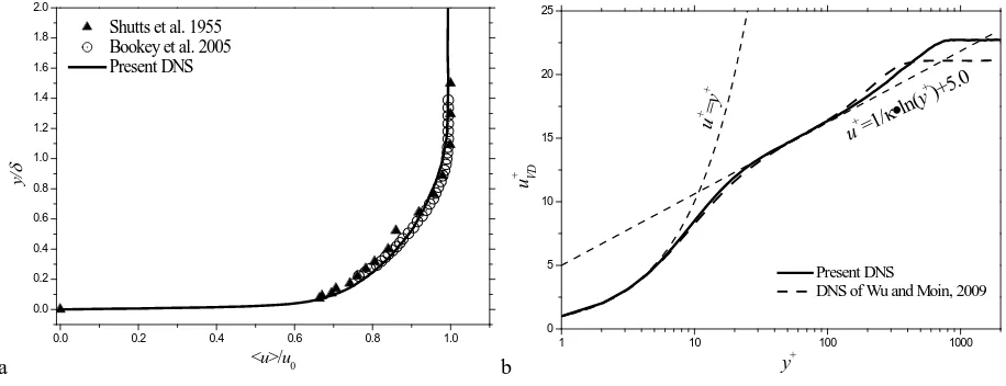
The mean velocity profiles are plotted in both outer and inner scalings in Fig. 3. The experimental measurements of Shutts et al. 26 and Bookey et al.27 are added in Fig. 3 (a) for comparison. The good agreements between the present DNS and experiments can be seen in the outer region of the boundary layer. In the inner scaling, 𝑢_𝑉𝐷+ is highly coincident with the classic law of wall in both the linear sub-layer and log-layer regions. A good agreement between the present DNS and incompressible DNS of flat-plate turbulent boundary layer of Wu and Moin 28 at Re𝜃 = 900 can also be found in Fig. 3 (b), except for the wake layer, where the present DNS shows

stronger strength of the wake component due to the higher Reynolds number used in the present case.

a

0.0 0.2 0.4 0.6 0.8 1.0 1.2 1.4 1.6 1.8 2.0

0.0 0.2 0.4 0.6 0.8 1.0

Shutts et al. 1955 Bookey et al. 2005 Present DNS

y

/

δ

<u>/u₀

b

1 10 100 1000

0 5 10 15 20 25

Present DNS

DNS of Wu and Moin, 2009

u

+ VD

y+ u

+ =y +

u+=1/ κ•ln(y

+₎₊₅.0

Fig. 3. Mean velocity profile in (a): outer scaling and (b): inner scalings at x=9.5. κ=0.41 is the von Kármán constant.

0.0 0.2 0.4 0.6 0.8 1.0 1.2 1.4 1.6 1.8 2.0

0.0 0.2 0.4 0.6 0.8 1.0 1.2 1.4 1.6 1.8 2.0

Present DNS Shutts et al. 1955 Pirozzoli et al. 2004

ρu/ρ₀u₀

T/T₀

y

/

δ

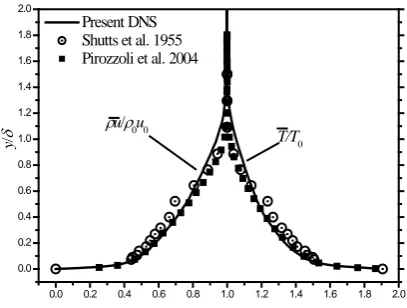
Fig. 4. Profiles of mean temperature and mass flux at x=9.5.

The mean wall pressure in the interaction region is shown in Fig. 5, together with the experimental data of Dupont et al. 30 at two closest flow conditions (M=2.3, α=32.4 and α=33.2), where 𝑋∗and 𝑃∗are defined in the same way as Dupont et al. 30, i.e. 𝑋∗ = (𝑥 − 𝑋₀)⁄𝐿_𝑆, 𝑃∗ = (𝑝̅ − 𝑝1) (⁄ 𝑝2− 𝑝1) , where 𝑋0 is the mean position of the reflected shock foot, 𝐿𝑆 is the length of

the interaction zone, 𝑝₁ and 𝑝₂ are the pressure upstream and downstream of the impinging shock deduced from the inviscid theory.

-1.0 -0.5 0.0 0.5 1.0 1.5 2.0 2.5

-0.5 0.0 0.5 1.0 1.5 2.0 2.5

Present DNS

Experiment of Dupont et al. at Ma=2.3, α=32.4Ο Experiment of Dupont et al. at Ma=2.3, α=33.2Ο

P

*

X*

Fig. 5. Mean wall pressure distributions in comparison with experiments.

It can be seen that the mean wall pressure of the present DNS matches well with the measurement data. The predicted wall pressure is increased smoothly, because the compression in the near-wall region is carried out by a series of compression waves due to strong inviscid-viscous interactions.

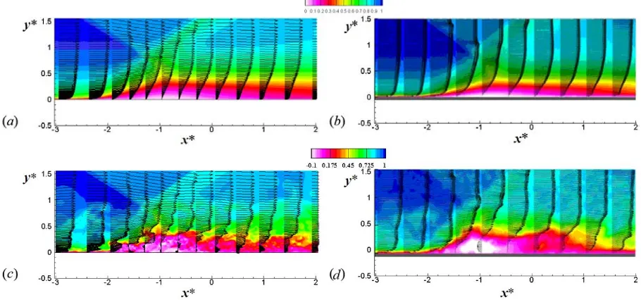
Fig. 6. Mean (a, b) and instantaneous (c, d) streamwise velocity and velocity vector s of present DNS (a, c) and PIV measurements of Humble et al. [2] (b, d).

It can be seen from Fig. 6 that DNS results and PIV measurements are very similar in terms of mean and instantaneous flow patterns, including the thickening of the boundary layer after interacting with the shock-wave, the formation of the mixing layer during the interaction as well as the complex instantaneous reverse flow in the interaction region. Both mean flows show small separation; however, from Fig. 6 (c, d), we can see the instantaneous flow separation happens in much larger region than that of the mean flow, which indicates the strong unsteadiness of the flow separation. Comparing with the PIV measurements, the DNS captures more flow details in the near-wall and the interaction regions due to its higher spatial resolution.

Fig. 7. Velocity fluctuation intensities in the interaction region, �〈𝒖′′𝒖′′〉 (a, b) and 𝟑�〈𝒗′′𝒗′′〉 (c, d) normalized with the velocity in the incoming flow of the present DNS (a, c) and PIV measurements of Humble et al. [2] (b, d).

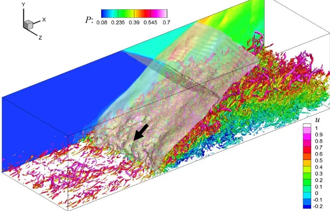
The instantaneous coherent structures are visualized in Fig. 8 by using the iso-surface of the swirling strength𝜆_𝑐𝑖 33 equaling to 0.5% of its global maximum. The coherent structures are well resolved by using the optimized MP7-LD scheme and the shock-wave is also well captured. The dramatic change in turbulence structures while passing through the shock-wave can be observed. In the undisturbed turbulent boundary layer, the streamwise elongated coherent structures in the near wall region, known as horseshoe vortex or hairpin vortex34 are predominant. After interacting with the shock-wave, the turbulence is detached from the wall, resulting in a thicker layer with much chaotic characteristics, which indicates the change of the turbulence production mechanism from wall-bounded turbulence to free shear-layer turbulence. The large-scale deformation of the impinging shock-wave surface can also be seen (pointed with an black arrow), which is similar with the observation by Priebe et al.4

Fig. 8. Coherent structures visualized using iso-surface of 𝝀_𝒄𝒊, rendered with the instantaneous streamwise velocity. The shock surface is visualized by using the iso-surface of the pressure gradient and a slice of pressure field is also shown

validate a DNS by checking the balance of the TKE transport equation. The TKE transport equation is expressed as,

𝜕0.5𝜌�〈𝑢_𝑘′′𝑢_𝑘′′〉

𝜕𝑡 =𝐶+𝑇+𝑃+𝑉 − 𝜀+𝐾, (1)

where, 𝐶= − 𝜕

𝜕𝑥_𝑗�0.5𝜌̅〈𝑢𝑗〉〈𝑢′′𝑘𝑢𝑘′′〉� is the advection term, 𝑇= − 𝜕

𝜕𝑥_𝑗�0.5𝜌̅〈𝑢𝑖′′𝑢𝑖′′𝑢𝑗′′〉+𝑝�������′𝑢𝚥′′ is the

turbulent transport term, 𝑃= −𝜌̅〈𝑢_𝑖′′𝑢_𝑗′′〉𝜕〈𝑢𝑖〉

𝜕𝑥𝑗 is the production term, 𝑉 =

𝜕 𝜕𝑥𝑗�𝜏𝚤𝚥

′ _𝑢𝚤′′

�������� is the viscous

diffusion term, 𝜀 = 𝜏_𝚤𝚥′ 𝜕𝑢𝚤′′

𝜕𝑥𝚥

��������

is the dissipation term and 𝐾 =𝑝′ 𝜕𝑢𝚤′′

𝜕𝑥𝚥

��������

+𝑢���� �𝚤′′ 𝜕𝜏_𝜕𝑥����𝚤𝚥_𝑗 −_𝜕𝑥𝜕𝑃�_𝑖� is the term

accounting for the direct effect of compressibility through pressure–dilatation correlation and mass diffusion .

The distributions of TKE budgets normalized with 𝜌_𝑊2𝑢_𝜏4⁄𝜇_𝑊 at 𝑥∗ =−3 are shown in Fig. 20. It can be seen that, all terms are distributed complicatedly in the interaction zone. The production and dissipation terms are greatly increased in the mixing layer formed in the interaction region, in which turbulence is dominated by some large-scale coherent structures as shown in Fig. 19. The strong TKE production in the mixing layer is balanced by the turbulent transport and dissipation terms. The viscous diffusion term is restricted in the very near-wall region and responsible for the near-wall TKE transport. The term K is effective in regions with shock-waves and compression waves, where the compressibility is strong.

a b

c d

e f

Fig. 9. Turbulence kinetic energy budget terms. (a): C, (b): T, (c): P, (d): ε, (e): V, (f): K.

near-wall region, the turbulent transport term transports TKE form high production region towards the wall and the near-wall TKE transport is further accomplished by the viscous diffusion term.

In the interaction and the following recovery regions, the property of the TKE transport equation becomes more complicated, which means the strong equilibrium of the turbulence. At

𝑥∗_{= −0.21, the peak of the turbulence production moves away from the wall, which indicates the}

change of the mechanism of the turbulence mechanism from wall turbulence to free-shear turbulence. The dissipation term also has a peak in the free-shear layer, which balances a part of the TKE production. The turbulent transport terms further balances the reset of the production by transport TKE towards the wall. The near-wall TKE transport is done by the almost equally contributions from turbulent transport and viscous diffusion.

In the recovery region, the outer peak of the production term decrease, due to the decay of the free-shear layer and the near-wall peak rises, which indicates the regeneration of the wall turbulence. The other terms also recovery towards the status in the undisturbed boundary layer, which mean the evolution of the boundary layer towards the equilibrium status.

a

0 10 20 30 40 50 60 70 80 90 100

-0.30 -0.25 -0.20 -0.15 -0.10 -0.05 0.00 0.05 0.10 0.15 0.20 0.25

0.30 C

T P V −ε K Balance B ud ge t/ ( ρ

2uW

4/µτ

W

)ref

y+ Lines: Present DNS

Scatters: Database of Pirozzoli & Bernardini (2011)

b

1 10 100 1000

-0.2 -0.1 0.0 0.1 0.2 C

T P

V −ε

K Balance

B u d g et /( ρ

2uW

4/µτ

W

)ref

y+ _c

1 10 100 1000

-0.2 -0.1 0.0 0.1 0.2 C

T P

V -ε

K Balance

B u d g et /( ρ

2uW

4/µτ

W

)ref

y+

Fig. 10. Turbulence kinetic energy balance at (a):𝑥∗=−3, (b): 𝑥∗=−0.21 and (c): 𝑥∗= 9.

Although the TKE budget relation changes dramatically when passing through the shock-wave, the balance of all terms is well preserved, which proves the effectiveness of the present numerical method in DNS of turbulent flow with shock-waves and flow separations.

3.2. 3D SWTBLI

of the wall pressure distribution also indicates the appearance of the secondary reattachment. Therefore, the pattern of wall streamlines of present case is coincident with that of the regime VI in the regime map of Zheltovodov and Knight17 at same similar Mach number and deflection angle.

Fig. 11. Mean skin-friction-line at the bottom wall. The red and green lines present S1 and the inviscid shock.

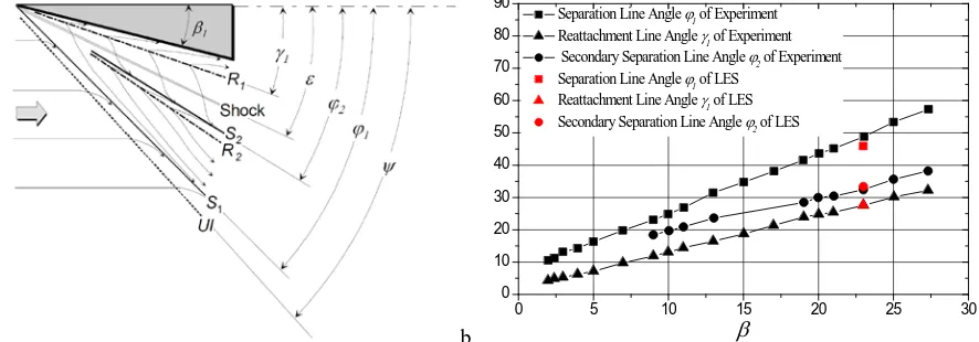
The comparisons of the angle of the separation line S1, the reattachment R1 and the secondary separation line S2 between the experiment measurements of Schülein and Zheltovodov35 and present LES are shown in Fig. 12. The agreement between the present LES and experiments is satisfactory.

a b

0 5 10 15 20 25 30

0 10 20 30 40 50 60 70 80 90

Separation Line Angle ϕ

1 of Experiment Reattachment Line Angle γ₁ of Experiment Secondary Separation Line Angle ϕ

2 of Experiment Separation Line Angle ϕ

1 of LES Reattachment Line Angle γ₁ of LES Secondary Separation Line Angle ϕ

2 of LES

β

Fig. 12. The definition of the angles of the separation and reattachment lines (a) and their distributions in the experiment and present LES (b)

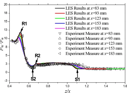
The wall pressure distributions at the cross sections of x=83mm, x=93mm, x=123mm, x=153mm and x=183mm are compared with the measurements of Schülein and Zheltovodov35 in Fig. 13, from which we can see the good agreement of the LES prediction and the experimental measurements. The separation and reattachment lines can be reflected from the local peaks of the wall pressure distribution. Although the secondary reattachment R2 is not so evidently from the skin-friction-line topology, it can be seen clearly from the wall pressure distribution at x=183 mm.

S1

R1 S2

0.4 0.6 0.8 1.0 1.2 1.4 1.6 -3 0 3 5 8 10 13 15 18 20 S1

LES Results at x=83 mm LES Results at x=93 mm LES Results at x=123 mm LES Results at x=153 mm LES Results at x=183 mm Experiment Measure at x=83 mm Experiment Measure at x=93 mm Experiment Measure at x=123 mm Experiment Measure at x=153 mm Experiment Measure at x=183 mm

pW / p∞ z/x R1 S2 R2

Fig. 13. Wall pressure distributions at several x-slices

According to previous researches, the “Virtual Conical Origin” (VCO) and the Spherical coordinate system (𝑅,𝛽,𝜑) is an appropriate coordinate frame to study these flows. In the present study, the position of VCO is at (-22.57mm, 0mm, -14.91mm).

The numerical schlieren 𝑟𝑛𝑠 and pressure gradient magnitude |∇𝑝| is used to analyze the shock structures. 𝑟𝑛𝑠 is calculated according to the formula, 𝑟𝑛𝑠= 𝑐₁𝑒−𝑐2(|∇𝜌|−|∇𝜌|𝑚𝑖𝑛) (|⁄ ∇𝜌|−|∇𝜌|𝑚𝑎𝑥)_,

where |∇𝜌| =�𝜕𝜌

𝜕𝑥𝑖

𝜕𝜌

𝜕𝑥𝑖, 𝑐1 = 0.8 and 𝑐2 = 10. |∇𝑝| is define as |∇𝑝| =�

𝜕𝑝 𝜕𝑥𝑖

𝜕𝑝

𝜕𝑥𝑖 and is normalized

with 𝑝_∞⁄𝛿₀, where 𝛿₀ is the nominal boundary layer thickness of the incoming flow.

The instantaneous 𝑟𝑛𝑠 and |∇𝑝| on the section at 𝑅 = 226.3𝑚𝑚 (𝑥= 183.7𝑚𝑚 at the surface of fin) is shown in Fig. 14, from which we can see clearly the 𝜆-shock system, which is composed with the main shock, the front shock (separation shock) and the rear shock. The rear and front shock legs meet the main shock at the “triple point”, and the rear shock has stronger strength than the front shock. A slip line is emitted from the triple points and a jet structures bounded by the slip line is then formed. The jet turns around the separation vortex and impinges to the wall at the mean reattachment line R1. At the impingement, a part of the jet penetrates the separation vortex, and becomes the reverse flow. Two separated regions with shocklets can be identified. Firstly, some shocklets can be observed between the rear shock and the slip line. Then shocklets are suppressed due to the Prandtl-Meyer expansion of the turning of the jet. Further downstream, the expansion fan reflects from the slip line as compression waves, which occasionally coalesce and form shocklets again, and the final shocklet becomes a normal shock that terminates supersonic jet prior to impingement. The expansion waves and shocklets can be seen more clearly in the map of |∇𝑝|. From Fig. 14 (b), some shocklets can also be founded beneath the front and rear shock and in the reverse flow. Further downstream, the shocklets beneath the front and rear shock will coalesce onto the front and rear chock, which is the same as the process in the two dimensional SWTBLI36,37. The shocklets in the reverse flow are located near S2-R2, which should be responsible for the secondary flow separation.

a

b

Fig. 14. Instantaneous numerical schlierenc and pressure gradient field (b) on the 3-D spherical arc section at 𝑹=

𝟐𝟐𝟔.𝟑𝐦𝐦

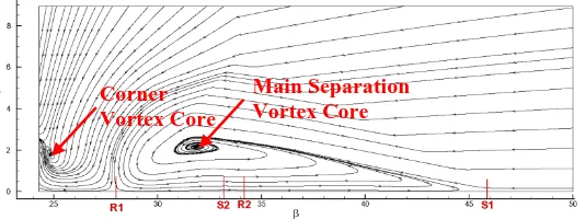
The streamlines �𝑢_𝛽,𝑢_𝜑� on the 3-D spherical arc section at R=226.3 mm are presented in Fig. 15. Unlike the closed configuration of the streamlines in the 2D separation bubble, the streamlines in Fig. 15 spiral around two focuses into which they disappear, therefore, present the 3D characteristic of the present flow separation. The two focuses are respectively the main separation vortex core and the corner vortex core.

Fig. 15. Mean streamlines �𝒖_𝜷,𝒖_𝝋� on the 3-D spherical arc section at 𝑹=𝟐𝟐𝟔.𝟑𝐦𝐦.

The streamlines originating from different values of y are shown in Fig. 16. It can be seen that, the streamlines from different heights presents different structures. The streamlines originating from the near-wall region (Fig. 16(a) presents a spiral structure around the separation vortex core. With the increase of the origination position (Fig. 16 (b), the streamlines directly enter the reversal flow, rather than through the vortex core. Further increase the height (Fig. 16 c), some of the streamlines

Front Shock Main Shock

Rear Shock Slip Line

Free Shear Layer

Jet Shocklets

Normal Shock

Shocklets

Normal Shock

Shocklets Reverse Flow

Main Separation Vortex Core Corner

go into the corner region, which indicates the existence of the corner vortex. The streamlines out of the boundary layer will not become the reversal flow; instead, they impinge to the mean attachment line R1 and move towards the surface of the fin.

a b

c d

Fig. 16 . Streamlines originating from y=2mm (a), y=4mm (b), y=6mm (c) and y=10 mm (d). The color stands for 〈𝒖〉

The mean stagnation pressure, static pressure and conical-cross Mach number 𝑀_𝑛 are presented in Fig. 17, from which, we can see the jet flow with high level of stagnation pressure rolling around the vortex core. The jet is supersonic initially and gets accelerated during the expansion process. The supersonic jet is terminated by the interaction with the normal shock and it further penetrates underneath the main vortex into the near-wall separation region and gets accelerated to supersonic (Fig. 17 c) again. Near the impinging location R1, the density and pressure get high (Fig. 17 (b), and the high pressure drives the flow to the fin’s surface and its reverse direction. Near the secondary separation line S2, the adverse pressure gradient can be seen, which should be attributed to the shocklets and the normal shock (as shown in Fig. 14 (b) in this region. The adverse pressure gradient should be the reason for the secondary flow separation. After S2, the reversal jet is detached from the wall, just like the main flow separation.

a b

c

Fig. 17. Distributions of: (a) the stagnation pressure, (b) the static pressure, and (c) the conical-cross Mach number𝑴_𝒏 , on the section at 𝑹=𝟐𝟐𝟔.𝟑𝐦𝐦. The black thin line in c) denotes the contour line of 𝑴_𝒏=𝟏.

From the instantaneous fluctuation 𝑢_𝑅′′ on the 3-D spherical arc section of x=35 mm shown in Fig. 18, the turbulent structures can be further investigated. Five zones can be distinguished according to the characteristics of turbulent structures. The first zone includes the undisturbed boundary layer attached to the bottom wall and surface of the fin, where the turbulent structures are the classic quasi-streamwise horseshoe vortex attached to the wall40. Another zone is the main free-shear zone, in which the turbulence is some large-scale turbulent structures (denoted with 2 in Fig. 18) with strong fluctuant energy detached from the wall. The turbulent structures in this zone are similar with those in the mixing layer, in which the flow is also dominated by the free shear41. The third zone is the edge of the jet, in which the flow is also dominated by the free shear flow and some large-scale turbulent structures. The difference with the second zone is that, the jet flow is not fully turbulent in it beginning part. Therefore, we can observe the transition process and the generation of large-scale structures by the Kelvin–Helmholtz instability as shown in the instantaneous schlieren picture in Fig. 14. The forth zone is the reverse flow, where some quasi-streamwise structures existence. The structures in this zone is similar with the wall turbulence in the first zone, but the structures are restrained in a thin layer close to the wall, therefore no large-scale structures, such as the horseshoe vortex heads, can be located. The fifth zone is the low-turbulent zone, which includes the core of the jet and a gap between the second zone and the forth zone. The flow in the fifth zone is quiet and less organized, just like the close separation bubble in the 2D SWTBLI, where the flow is filled with less organized fluid.

a

b c d

Fig. 18 Instantaneous 𝒖_𝑹′′ on the section at 𝑹=𝟐𝟐𝟔.𝟑𝐦𝐦. (b), c) and d) are the zoomed picture of local flow structures in (a). The arrow stands for the 2D vector of �𝒖_𝜷′′,𝒖_𝝋′′�. 1 indicates the undisturbed wall turbulent structure,

2 indicates for the large scale vortex in the shear layer, 3 indicates the large-scale structures in the jet, 4 indicates the regenerated wall turbulent structures.

The vorticity fluctuation in the R direction 𝜔_𝑅′′ on the section of 𝑅 = 226.3mm are present in Fig. 19, in which 𝜔_𝑅′′ is normalized with 𝑢₀⁄𝛿₀ and (𝑢₀⁄𝛿₀)2. Since the vorticity is closely related

4 2

3 4

1 2

to the turbulent structures, the above mentioned five zones (as marked in Fig. 19 (a), are more distinguishable in Fig. 19.

Fig. 19 . Instantaneous field of vorticity fluctuation 𝝎_𝑹′′on the section at 𝑹=𝟐𝟐𝟔.𝟑𝐦𝐦.

The structures in the zone 1 are the combination of small-scale strong fluctuations in the near-wall region and large-scale weaker fluctuations in the outer region. The turbulence in zone 2 is also very strong, and these fluctuations are weakened with the diffusion of the free-shear layer. The zone 3 only occupies only a slim region, in which the transition of the shear layer by Kelvin–Helmholtz instability can be seen. The zone 4 is a thin layer attached to the wall, but the fluctuations in it are strong. The zone 5 present a gap between zone 2, zone 3 and zone 5, and the space of the gap become larger with the further development of the shear layer, due to the quasi-conical property of the flow. The transition process can be seen in the zone 3. The intensity and the length scale of the structures in this zone increase with the development of the jet flow, and finally these structures enter the core region and the reverse flow after the impingement of the jet. Besides the 5 zones, the turbulence in the corner region also presents complex property, due to the complex flow mechanism in this region.

The turbulent kinetic energy (TKE) 𝐾=1

2�〈𝑢′′𝑢′′〉� +〈𝑣′′𝑣′′〉� +〈𝑤′′𝑤′′〉� � on the section of 𝑅 = 226.3mm is presented in Fig. 20. Consistent with the previous analysis, TKE presents high values in the zone 2. The zone 3 also has a certain level of TKE and the turbulent energy spreads outwards with the transition of the jet flow. In the zone 5, the level of TKE is lower than its circumstance. Near S2, the increase of TKE and the thickening of the near-wall shear-layer can be seen, which can be seen more clearly in the zoomed figure Fig. 20 (b). The amplification mechanism is also the activation of turbulence by the adverse pressure gradient, which is similar with that of the amplification of turbulence at S1. However, the amplification of turbulence at S2 is only restrained in a limited region, therefore, no large-scale separation region and detached free-shear layer can be observed. Passing through S2, the TKE decreases to the level before the secondary separation.

a b

Fig. 20. Turbulent kinetic energy on the section at 𝑹=𝟐𝟐𝟔.𝟑𝐦𝐦, normalized with the square of the wall friction velocity 𝒖_𝝉𝟐 at the inlet.

1 1

2 3

4

4. Concluding Remarks

The 2D impinging shock-wave/flat-plate boundary layer interaction and 3D SWTBLI of a Mach 5 flow passing through a 23° single-fin are studied by using DNS and LES respectively. The results of both cases are well validated and the data are then analyzed to investigate the flow property and the turbulence characteristic in the 2D/3D SWTBLI. Some conclusions can be reached,

1. In the 2D SWTBLI, a mixing layer is formed with the flow separation and the turbulence characteristic changes from equilibrium wall-turbulence to non-equilibrium free-shear turbulence. The TKE balance property is changed greatly in the interaction region, of which the production core is shifted from the near-wall region to the core of the mixing layer. The balance of TKE transport equation is well preserved in the present DNS, which proves the effectiveness of the used numerical method.

2. By analyzing the mean skin-friction-line with the Critical Point Theory, the flow in 3D SWTBLI is separated at the foot of the separation shock and reattached near the corner region. The secondary flow separation and reattachment lines can also be identified, which is consistent with the regime characteristic of Zheltovodov and Knight17. The streamlines lift at the separation line and fall off near the fin’s surface, which transport the fluid with high energy to the near wall region. In the separation vortex, the streamlines curls around the separation vortex core, and generate the reverse flow beneath the separation vortex.

3. In 3D SWTBLI, a free shear layer with strong mean shear strength and low kinetic energy is generated when flow is detached near the mean separation line. The free shear layer is deflected away from the wall from the separation line and the vortex core is therefore formed. A jet flow originating from the triple point, rolls tightly around the vortex core and impinges to the wall at the mean reattachment line. The supersonic jet penetrates into the reverse flow beneath the separation vortex and brings fluids with high energy to the reverse flow. The supersonic jet is terminated by interaction with a normal shock and then impinges to the bottom wall near the mean reattachment line, inducing high level of pressure there. The high pressure drives the reverse flow to supersonic, which is then terminated by another interaction with a normal shock inside the reverse flow, and causes the secondary flow separation.

4. The great change of turbulence characteristic can be found in the interaction zone of the 3D SWTBLI. The flow field can be categorized into 5 zones according to the characteristics of turbulent structures. Zone 1 is the undisturbed wall turbulence in the upstream boundary layer. Zone 2 is the separated free shear layer, which contains some large-scale structures with high fluctuant energy. Zone 3 is the slip line, which is also the edge of the jet. The turbulence in this zone is also dominated by the free shear but the flow is still in the process of transition. Zone 4 is the reverse flow, which is also characterized by wall-turbulence, but only restrained in a thin layer attached to the wall. The wall-turbulence is induced by the jet flow, which has strong kinetic energy and large-scale fluctuations. Zone 5 is the low-turbulent zone, which includes the core of jet and the gap between the zone 2 and zone 4.

Acknowledgments

REFERENCES

1. Dolling D.S., Fifty Years of Shock-Wave/Boundary-Layer Interaction Research: What Next? // AIAA J. 2001. Vol.

39. P.1517-1531.

2. Jammalamadaka A., Li Z., Jaberi F., Numerical Investigations of Shock Wave Interactions with a Supersonic

Turbulent Boundary Layer // Phys. Fluids. 2014. Vol.26. No. 056101.

3. Pirozzoli S., Bernardini M., Direct numerical simulation database for impinging shock wave/turbulent

boundary-layer interaction // AIAA J. 2011. Vol.49. P.1307-12.

4. Priebe S., Wu M., Martin M.P., Direct Numerical Simulation of a

Reflected-Shock-Wave/Turbulent-Boundary-Layer Interaction // AIAA J. 2009. Vol. 47. P. 1173-1185.

5. Pirozzoli S., Grasso F., Direct numerical simulation of impinging shock wave/turbulent boundary layer interaction

at M=2.25 // Phys. Fluids. 2006. Vol. 18. No.065113.

6. Zheltovodov A.A., Some advances in research of shock wave turbulent boundary-layer interactions // 44th AIAA

Aerospace Sciences Meeting and Exhibit. Reno, Nevada. 2006. AIAA Paper 2006–0496.

7. Schülein E., Skin-Friction and Heat Flux Measurements in Shock/Boundary-Layer Interaction Flows // AIAA J.

2006. Vol. 8. P. 1732-1741.

8 . Zheltovodov A.A., Maksimov A.I., Shevchenko A.M., Topology of three-dimensional separation under the

conditions of symmetric interaction of crossing shocks and expansion waves with turbulent boundary layer // Thermophysics and Aeromechanics. 1998. Vol. 5. P. 293–312

9 . Dolling D.S., Bogdonoff SM. Upstream influence in sharp fin-induced shock wave/turbulent boundary layer

interaction // AIAA J. 1983. Vol. 21. P. 143–145.

10. Settles G.S., Bogdonoff S.M., Scaling of two- and three-dimensional shock/turbulent boundary-layer interactions at

compression corners // AIAA J. 1982. Vol. 20. P. 782–279.

11. Kubota H., Stollery J.L., An experimental study of the interaction between a glancing shock wave and a turbulent

boundary layer // J. Fluid Mech. 1982. Vol. 116. P. 431–458.

12. Panov Y.A., Interaction of a three-dimensional shock wave with a turbulent boundary layer. Fluid Dynamics

Research // 1966. Vol. 1. P. 131–133.

13. Salin A., Yao Y.F., Lo S.H., Zheltovodov A.A., Flow Topology of Symmetric Crossing Shock Wave Boundary

Layer Interactions // 28th International Symposium on Shock Waves. 2012. P. 425–31.

14. Knight D., Gnedin M., Becht R., Zheltovodov A.A., Numerical simulation of crossing

shock-wave/turbulent-boundary-layer interaction using a two-equation model of turbulence // J. Fluid Mech. 2000. Vol. 409. P. 121–147.

15. Panaras A.G., Numerical Investigation of the High Speed Conical Flow Past a Sharp Fin // J. Fluid Mech. 1992.

Vol. 236. P. 607–633.

16. Hung C.M., MacCormack R.W., Numerical solution of three-dimensional shock wave and turbulent

boundary-layer interaction // AIAA J. 1978. Vol. 16. P. 1090–1096.

17. Zheltovodov A.A., Knight D.D., Ideal-Gas Shock-Wave-Turbulent Boundary-Layer Interactions in Supersonic

Flows and their Modeling: Three-Dimensional Interactions // In: Babinsky H, Harvey JK, editors. Shock Wave-Boundary-Layer Interactions. London: Cambridge University Press; 2011. P. 202-58

18. Moin P., Squires W., Cabot W., Lee S.A., A dynamic subgrid-scale model for compressible turbulence and scalar

transport // Phys. Fluid A. 1991. Vol. 3. P. 2746 -2757.

19. Ghosal S., Lund T.S., Moin P., Akselvoll K., A dynamic localization model for large-eddy simulation of turbulent

flows // J Fluid Mech. 1995;286:229-55.

20. Fang, J. Li, Z. and Lu, L. An Optimized Low-Dissipation Monotonicity-Preserving Scheme for Numerical

Simulations of High-Speed Turbulent Flows // J. Sci. Comput. 2013. Vol. 56. P. 67-95.

21. Suresh, A. and Huynh, H.T. Accurate Monotonicity-Preserving Schemes with Runge–Kutta Time Stepping // J.

Comput. Phys. 1997. Vol. 136. P. 83-99.

22. Lele, S.K. Compact Finite Difference Schemes with Spectral-Like Resolution // J. Comput. Phys. 1992. Vol. 103. P.

16-43.

23. Gottlieb, S. and Shu, C.W. Total Variation Diminishing Runge-Kutta Schemes // Mathematics of Computation.

1998. Vol. 67. P. 73-85.

24. Rai, M.M., Moin, P., Direct Numerical Simulation of Transition and Turbulence in a Spatially Evolving Boundary

Layer // J. Comput. Phys., 1993, 109:169-192.

25. Pirozzoli S., Grasso F., Gatski T.B., Direct Numerical Simulation and Analysis of a Spatially Evolving Supersonic

Turbulent Boundary Layer at M=2.25 // Phys. Fluids, 2004, Vol. 16. No. 3. P. 530-545.

26 . Shutts WH, Hartwig WH, Weiler JE., Final Report on Turbulent Boundary Layer and Skin Friction

Measurements on a Smooth, Thermally Insulated Flat Plate at Supersonic Speeds // Defense Research Laboratory; 1955; DRL-364.

27. Bookey P., Wyckham C., Smits A., New Experimental Data of STBLI at DNS/LES Accessible Reynolds Numbers

28 . Wu X., Moin P., Direct numerical simulation of turbulence in a nominally zero-pressure-gradient flat-plate boundary layer // J. Fluid Mech. 2009. Vol. 630. No. 5-41.

29. Shutts W.H., Hartwig W.H., Weiler J.E., Final report on turbulent boundary layer and skin friction measurements

on a smooth, thermally insulated flat plate at supersonic speeds // Defense Research Laboratory. 1955. DRL-364.

30. Dupont P., Haddad C., Debieve J.F., Space and time organization in a shock-induced separated boundary layer // J

Fluid Mech. 2006. Vol. 559. P. 255-77.

31 . Humble R.A., Scarano F., van Oudheusden B.W., Particle image velocimetry measurements of a shock

wave/turbulent boundary layer interaction // Exp. Fluids. 2007. Vol. 43. P. 173-183.

32. Humble R.A., Elsinga G.E., Scarano F., van Oudheusden B.W., Three-dimensional instantaneous structure of a

shock wave turbulent boundary layer interaction // J. Fluid Mech. 2009. Vol. 622. P.33-62.

33. Zhou J., Adrian R.J., Balachandar S., Kendall T.M., Mechanisms for generating coherent packets of hairpin

vortices in channel flow // J. Fluid Mech. 1999. Vol. 387. P. 353-396.

34. Adrian R.J., Meinhart C.D., Tomkins C.D., Vortex organization in the outer region of the turbulent boundary

layer // J. Fluid Mech. 2000. Vol. 422. P. 1-54

35 . Schülein, E., and Zheltovodov, A.A. Documentation of experimental data for hypersonic 3-D shock

waves/turbulent boundary layer interaction flows // DLR Gottingen. 2001. IB 223 – 99 A 26.

36 . Loginov, M.S., Adams, N.A. and Zheltovodov, A.A. Large-Eddy Simulation of

Shock-Wave/Turbulent-Boundary-Layer Interaction // J. Fluid Mech. 2006. Vol. 565 P. 135-169.

37 . Wu, M., and Martín, M.P. Direct Numerical Simulation of Supersonic Turbulent Boundary Layer Over a

Compression Ramp // AIAA J. 2007. Vol. 45. No. 4. P. 879-889

38. Alvi, F.S. and Settles G.S. Structure of swept shock wave/boundary layer interactions using conical shadowgraphy

// AIAA Paper 90–1644. 1990.

39. Alvi, F.S. and Settles G.S., A physical model of the swept shock/boundary-layer interaction flowfield // AIAA

Paper 91–1768. 1991.

40. Ringuette, M.J. Wu, M. and Martin, M.P. Coherent Structures in Direct Numerical Simulation of Turbulent

Boundary Layers at Mach 3 // J. Fluid Mech. 2008. Vol. 594. P.59-69.

41. Moser, R.D., and Rogers, M.M. Coherent structures in a simulated turbulent mixing layer // Eddy Structure