The Influence of Search Components and Problem
Characteristics in Early Life Cycle Class Modelling
J.E. Smith∗, C.L. Simons
Department of Computer Science and Creative Technologies, University of the West of England, Bristol, UK
∗Corresponding author
Email address: [email protected](J.E. Smith)
URL: http://www.bit.uwe.ac.uk/~jsmith(J.E. Smith),
The Influence of Search Components and Problem
Characteristics in Early Life Cycle Class Modelling
J.E. Smith∗, C.L. Simons
Department of Computer Science and Creative Technologies, University of the West of England, Bristol, UK
Abstract
This paper examines the factors affecting the quality of solution found by meta-heuristic search when optimising object-oriented software class models. From the algorithmic perspective, we examine the effect of encoding, choice of components such as the global search heuristic, and various means of incorporating problem- and instance-specific information. We also consider the effect of problem characteristics on the (estimated) cost of the global optimum, and the quality and distribution of local optima.
The choice of global search component appears important, and adding problem and instance-specific information is generally beneficial to an Evo-lutionary Algorithm but detrimental to Ant Colony Optimisation. The effect of problem characteristics is more complex. Neither scale nor complexity have a significant affect on the global optimum as estimated by the best solution ever found. However, using local search to locate 100,000 local optima for each problem confirms the results from meta-heuristic search: there are pat-terns in the distribution of local optima that increase with scale (problem size) and complexity (number of classes) and will cause problems for many classes of meta-heuristic search.
Keywords: Search-Based Software Engineering, Class Modelling,
Evolutionary Algorithms, Ant Colony Optimisation, Memetic Algorithms
∗Corresponding author
Email address: [email protected](J.E. Smith)
URL: http://www.bit.uwe.ac.uk/~jsmith(J.E. Smith),
1. Introduction
The task of class modelling within early cycle object orientated software engineering is often poorly tackled by humans. Issues such as scale and complexity pose significant issues, but the ongoing history of software failures shows that their relative effect in creating difficulties is not well understood. Recent research has demonstrated that this task, also referred to as the Class Responsibility Assignment Problem, can be successfully tackled by posing it as a search problem. For the sake of brevity we will hereafter refer to it as “class modelling”, with the restriction to the context of the early stages of the development life cycle being taken as read. The “Search Based Software Engineering” (SBSE) approach to class modelling has been illustrated using both Evolutionary Algorithms (EA) and Ant Colony Optimisation (ACO) to perform the underlying search. Each of these outperforms methods based on a single improving solution, and has been shown to display strengths and weaknesses - both in terms of optimisation performance, and of how easily “standard” algorithms can be applied to the domain. However, three major questions remain unanswered. The first is whether the problems caused by scale and complexity are a result of human limitations, or do they also exist when the task is formulated for automated search? The second is how task-specific information can be incorporated at various levels to manage the global-local search trade-off, and aid search by avoiding breaking constraints. The third is the identification of design problem characteristics that make automated search harder, to inform the creation of a richer and more rigorous suite of benchmark problems than currently exists.
Our contention is that because of its complex, subjective nature, class modelling should be tackled via interactive search, augmented with a sur-rogate fitness function to prevent user fatigue. Therefore ideally the choice of search method should consider the ease with which it can support users’ input via actions such as “freezing” satisfactory parts of designs. Previously [19, 20] we compared ACO and EAs as global search algorithms for this task, concluding that performance issues aside, there are practical reasons for pre-ferring to use some heuristics. For example, in an ACO “freezing” of partial solutions can be simply achieved via direct changes to the pheromone ta-ble. In contrast, it would necessitate manipulation of an EA’s recombination and mutation operators on-the-fly, although progress has been made in this direction by interleaving phases of human manipulation and evolution [27].
performance, so understanding the latter is vital before we can disregard it, and clearly algorithmic simplicity cannot be a substitute for poor perfor-mance. Initial investigations [20] showed that in their canonical form EAs outperformed ACO. In a recent paper we extended this work to incorpo-rate the effect of local search to create two different examples of the class of memetic algorithms (MAs) [9]. Those preliminary studies still showed that the MAs using evolution as the global search component (hereafter M-EAs) found higher quality solutions than those based on ACOs (hereafter M-ACO). It should be noted that for the sake of “fairness” the ACOs in those papers did not make any use of heuristic or instance-specific information.
This paper extends that study to examine the effect of different ways in which information can be incorporated within meta heuristic search. Each of these creates its own bias in determining the probability distribution func-tions that govern the generation of candidate solufunc-tions. From the SBSE perspective it is important to gain an understanding of how these impact on performance as class modelling problems vary in scale and complexity. In order to provide some insights into these issues, Section 2 provides a brief background to previous research in this problem domain, and the re-lationship between class modelling and the more abstract problem of graph partitioning. Section 3 describes the chosen representation, the global and local search components considered, and different ways in which problem-specific information can be incorporated. Section 4 describes the experimen-tal methodology used, then Section 5 describes, and Section 6 analyses the results obtained. Finally Section 7 summarises the findings and implications for SBSE in general, and early stage class modelling in particular.
2. Background
2.1. What Makes a Class Modelling Problem Hard?
relate to relevant concepts and information in the problem domain. There is evidence to suggest that act of early lifecycle class modelling is non-trivial and demanding to perform, not least due to the scale and complexity of the problem domain. For many problems the number of methods and attributes can run to hundreds, with a corresponding multiplicity of classes. Petre [13] has suggested that software design problems are often wicked: too big, too ill-defined, too complex for easy comprehension and solution. Sometimes the problems are only fully understood after they are solved. Solving such problems is rarely a matter of brute force or routine. Glass [7] goes further, suggesting that the scale and complexities of some software designs may be beyond human comprehension. There is also evidence that designers are blessed with varying degrees of modelling talent. Even for experienced mod-ellers, Glass notes that designer performance may vary from 28:1 from the best to the worst. Curtis [4] also notes a range in talent, observing that only super-designers can reason across the full breadth and depth of com-plex, ill-structured problems in order to fully consider the consequences and decisions of modelling decisions. From the field of education there is evidence that class modelling is difficult to learn. In a study of 740 undergraduates and 135 design problems, Svetinovic et al. [26] observe that with respect to concept identification, “some students just don’t get it”.
2.2. Search-Based Software Engineering
Search-Based Software Engineering (SBSE) is a well-established disci-pline, applied across the whole software development lifecycle [30]. Histor-ically, comparatively little focus has been directed to the upstream stages, although this is beginning to be addressed. Typically metrics relating to cou-pling and cohesion are used to guide meta-heuristic search of design spaces of object-oriented class models. Bowmanet al. [2] used a multi-objective EA to optimise designs for a number of pre-specified metrics, but only considered a single problem instance. Simons and Parmee [18, 17] applied interactive EAs, using linear regression to learn a surrogate fitness model combining cou-pling with a number of “elegance metrics” to approximate users’ subjective preferences for different problems. Working slightly later in the development life-cycle, Sievi-Korte et al.[15] used an M-EA, and Vathsavayi et al.[27] in-terleaved human and evolutionary adaptation of the usage of patterns.
Although any search algorithm could be used in SBSE, research effort has tended to concentrate on EAs. Previously we compared the use of ACOs and EAs for this problem [19, 20], concluding that given sufficient computational budget, global search via EAs was more effective at finding high quality so-lutions than that using ACO. When the computational budget was reduced (as is, for example, often the case in interactive search) the situation was re-versed. However, with both algorithms, and both representations examined, a major issue was dealing with the constraint that a valid class model should contain at least one attribute and at least one method. Those papers used penalty functions (all invalid models were given zero fitness) and the use of random regeneration of invalid solutions. Dealing more efficiently with this constraint would necessitate either a significant adaptation of the underlying global search heuristics, or the provision of a “repair” mechanism.
evo-lutionary framework, it is standard practice in ACO research and is readily incorporated, as will be shown in later sections.
2.3. Relationship to Graph Partitioning and Similar Problems
The creation of class models can be thought of as a process of grouping elements (attributes and methods) into classes, so that every class contains at least one element of each type. The initial description of the problem as captured via, for example, use-cases, specifies a number of “uses”. For ex-ample, in a sales application a method “create invoice” might make reference to attributes such as “customer-id”. Therefore it is natural to think of the combination of elements and uses as defining a graph G= (V, E) where the sets of methods M and attributesAare vertices (i.e., V =M∪A) and a use of attribute i∈A by a method j ∈M creates an edge eij ∈E.
While many different metrics have been proposed to capture some mea-sure of the quality of a software design, it is commonly recognised that a good design will exhibit high cohesion and loose coupling. Hence, uses tend to hap-pen within a class, and the usage of attributes from one class by methods of another is minimised. In terms of a graph structure this means dividing the vertices into a number of discrete partitions so that the number of edges between partitions in minimised.
This description makes the link between class modelling and graph parti-tioning clear. Some differences exist - for example, graph partiparti-tioning meth-ods assume all vertices are of the same type and in the most common form of “uniform graph partitioning” they explicitly try to minimise imbalance, usually with fixed number of partitions. Closely related “grouping” problems such as the multiple knapsack problems may consider the “cost” or “value” or a vertex, but still treat all as essentially of the same type. We note that requiring each class to contain at least one method and at least one attribute creates an extra constraint since not all vertices are of the same type.
Graph partitioning is NP-hard and has been extensively studied [1, 8]. A full review is beyond the scope of this paper, but it is notable that many successful recent applications use a form of spectral partitioning based on an adjacency graph (an alternative representation of the edge set), and re-peatedly bi-partition the graph and then its components. In Section 3.6 we describe the creation of a distance matrix to be used by the ACO, based on a generalisation of adjacency matrices.
repre-sentation. One active research question is whether it is possible, or indeed desirable, to avoid the explicit redundancy that comes from assigning arbi-trary labels to groups. A further problem is that even multiple-colony ACO models, wherein each colony forms a separate partition, use a permutation type representation by default. This introduces extra redundancy, since the many solutions corresponding to different permutations of the nodes in a partition are semantically identical. Section 3.5 describes a modification of ACO’s pheromone update mechanism to remove this redundancy.
3. Representation and Algorithms
This section briefly overviews the way in which class modelling is posed as a search problem, and the three search algorithms used in this paper.
3.1. Representation
In order to map readily onto freely available ACO source code, we borrow a representation commonly used for Vehicle Routing Problems. A solution is considered to be a permutation of a set of items, comprising the design elements plus “end-of-class” markers. If a problem has a attributes and m methods, to be grouped into up to c classes, the representation is then a permutation of size l =a+m+c−1. The value in the ith position denotes
the element that occurs in the ith place in the tour, where the attributes are
numbered from 1 toa, the methods froma+1 toa+mand the “end-of-class” markers froma+m+1 toa+m+c−1. Since the permutation for a candidate solution might contain adjacent end-of-class elements, crepresents an upper limit on the number of classes in any given solution, rather than a fixed value. When the representation of a solution is decoded to give the candidate class model, a simple arrayclass= [c1, . . . , ca+m] is constructed whosejth element
3.2. Evolutionary Algorithm
The EA chosen is a standard generational genetic algorithm. Parents are chosen by deterministic binary tournaments, with elitism so that the incum-bent replaces the least fit of the newly created offspring if better. Crossover was applied with probability 0.7. We do not provide a full algorithmic de-scription of the EA as this is a well known algorithm with many dede-scriptions online. Full details of the operators used can be found in [5]. Parameter values were determined by extensive preliminary testing. To examine the effect of in-class redundancy we investigated two different representations. The first was the permutation outlined above with length l = a+m−1, in which case we used Edge Recombination, and mutation randomly applied one of Swap, Insert and Invert operators. The second was a direct encod-ing of class labels to elements with a representation of length l = a +m and search space {1, . . . , c}a+m. In this case we used uniform crossover, and
mutation randomly chose a new allele value for each position applied. There is now a significant body of evidence in favour of the use of self-adaptive mutation rates (see, for example, [12]). Following one of the schemes proposed by Serpell and Smith [14], each individual contained an extra gene encoding the mutation probabilitypm, and we adopted the following method
for mutation of each offspring:
1. With probability 0.2 the encoded value of pm was changed to a new
value, selected uniformly at random from the fixed set of allowed values. 2. The value forpm was multiplied by the representation lengthl, and the
result truncated to an integer to give the number of mutation events. 3. The chosen mutation operator was then applied the number of times
determined in the previous step to randomly chosen positions.
A fixed set of ten mutation rates was defined aspm·l∈ {0.001,0.002,0.01,
0.02,0.1,0.2,1,2, M IN(0.25l,5), M IN(0.25l,10)}. A range of population sizes were used as detailed in Section 4.4.
3.3. Ant Colony Algorithm
these define the probability distribution function for the generation of new solutions. In each iteration N ants are each placed at random at a starting node and tours are independently created. To construct its tour, at each successive node i, the ant creates a list S of all the as-yet unvisited nodes. It then selects a next node j ∈S from the list with probability:
pmove(ij) =
Pα ij·H
β ij P
j6=i,j∈SPijα·H β ij
,if j ∈S
0 , otherwise.
(1)
After the ant has constructed a full solution its fitnessf is measured. If best denotes the least cost path for generation t, and {ij} ∈best is taken to mean that edge {ij} is traversed in that path, then the pheromone matrix M is updated at the end of each generation according to:
Pijt+1 = (
(1−ρ)·Pijt + 1/fbest ,if {ij} ∈best,
(1−ρ)·Pijt ,otherwise. (2)
The key factors which distinguish the MAX-MIN ACO are that the pheromone matrixP is initialised to its maximum value, is only updated with the information from the best ant per generation, and that the pheromone levels are truncated to a pre-specified range to avoid over saturation.
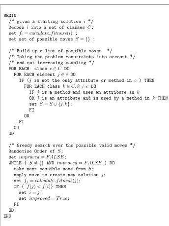
3.4. Local Search Algorithm
The single-step greedy local search algorithm in Fig. 1 was implemented. Using problem-specific information in terms of task constraints, the pertur-bation operator moves one element to a different class as long as it does not leave behind an invalid class. Taking account of instance-specific informa-tion, a method can only move to a “receiving” class that has an attribute that it uses and vice-versa. This last condition does not assure that the fitness of the neighbour is superior to that of the incumbent, but rules out evaluating some of the least fit neighbours - at least in terms of coupling. Together these restrictions greatly reduce the size of the neighbourhood that needs to be examined, and so make local search more efficient.
3.5. Problem Specific Heuristics: Modified Pheromone Update
As noted above, the permutation representation creates redundancy, since the order in which elements appear within a class is immaterial. The following modification to Eq. 2 was designed to remove this effect, by increasing the pheromone laid down between all pairs of members of the same class in the best solution, and reducing it for all out of class members. Usingclass∗[i] to denote the class label of element iin the best solution of a given iteration:
Pijt+1 =
(1−ρ)·Pijt + 1/fbest ,if i, j ≤a+m and class∗[i] =class∗[j],
(1−ρ)·Pijt −1/fbest ,if i, j ≤a+m and class∗[i]6=class∗[j],
(1−ρ)·Pijt ,otherwise.
Not shown here for reasons of space, are results using only the positive reinforcement (i.e., omitting the middle line of the equation above) which demonstrated worse performance.
3.6. Instance Specific Heuristic Information: Distance matrices
When applying ACO to routing problems such as the TSP, the heuristic matrix H can naturally encode for features such as the distance between nodes by setting Hij = 1/distance(i, j), to increase the probability of ants
BEGIN
/* given a starting solution i */
Decode i into a set of classes C;
set fi=calculate f itness(i) ;
set set of possible moves S={} ;
/* Build up a list of possible moves */
/* Taking the problem constraints into account */
/* and not increasing coupling */
FOR EACH class c∈C DO
FOR EACH element j∈c DO
IF (j is not the only attribute or method in c ) THEN
FOR EACH class k∈C, k6=c DO
IF j is a method and uses an attribute in k
OR j is an attribute and is used by a method in k THEN
set S=S∪ {j, k}; FI
OD FI OD OD
/* Greedy search over the possible valid moves */
Randomise Order of S;
set improved=F ALSE;
WHILE ( S6={} AND improved=F ALSE ) DO
take next possible move from S;
apply move to create new solution j;
set fj =calculate f itness(j); IF ( f(j)< f(i)) THEN
set i=j;
set improved=T rue;
[image:12.612.111.455.154.612.2]FI OD END
For each task, based on the use cases in the documentation and the numbering scheme above, an l×l matrix U was constructed with:
Uij =
1 i≤a, a < j ≤a+m, if method j uses attributei, 1 j ≤a, a < i≤a+m, if method i uses attributej, 0 otherwise.
Furthermore, since Uij is the number of one-step paths between elements i
and j, a useful result is thatUijn is the the number of length-n paths between i and j. We therefore calculate matrices Un for a range of values of n and
from these define a Distance Matrix D with elements Dij = M IN(n) such
that Uijn > 0. The heuristic information matrix H is thereafter defined as Hij = 1/Dij, for all non-zero Dij and zero otherwise.
In terms of class modelling, this means that if methodiuses attributes j and k, thenDij =Dik = 1 and Djk = 2. The same is true ifi is an attribute
used by methods j and k. We examined path lengths up to a distance of n = 10 - no problems examined had elements further apart.
4. Methodology
4.1. Quality Metrics
Many different quality measures have been proposed in the literature, and it remains an open question whether a multi-objective approach should be applied. However, it should be noted that the aim of class modelling is not to attain an approximation of the Pareto front since the extrema are of no interest. For example, one non-dominated solution always exists that achieves zero coupling by putting all elements into a single class. However, this goes against the whole spirit of object-orientated design, and in practice software designers deprecate this “anti-pattern”, as it tends to lead to low cohesion (amongst other problems)[3].
Several authors have pursued the concept of “design elegance” in this and other fields. We have recently proposed several metrics that directly reflect a sense of “elegance” in terms of a symmetrical distribution of attributes and methods in a design[17].
a spread of users correlated highly to those of a surrogate model comprising a simple linear regression of a few metrics. Moreover, when presented with the candidate solutions obtained by meta-heuristic search using this model, users reported high degrees of satisfaction. This suggests strongly that the designs created did make sense to the users, despite having been created without any semantic knowledge of the labels on various elements such as name,address,
booking etc.
Based on the regression co-efficients identified, we consider a single cost function (to be minimised) composed of two equally weighted elements:
fcomb = 0.5∗(fcbo+fnac) (3)
The first element is based on the Coupling Between Objects (CBO) measure. The cost is defined as the percentage of all uses that are “out of class”:
fcbo = 100·
P
i
P
j,class(j)6=class(i)Uij
P
i
P
j, Uij
. (4)
The second cost element is the Numbers Among Classes (NAC):
fnac=
100 6 ∗
σm 2 +
σa
2
(5)
where σm and σa denote the standard deviations across all classes of the
numbers of methods and attributes per class, truncated to the range [0,6]. The lower this value, the more symmetrical the appearance of attributes and methods among the classes in the design, hence it tends to counterbalance the effect of the CBO metric.
4.2. Performance Metrics
Given that ultimately we are concerned with the use of these search heuristics embedded in an interactive design tool, that we assume the use of a surrogate fitness measure, and that we do not know an “optimal” fitness for each instance, we compare different search algorithms according to their effectiveness and consistency in finding good solutions.
variable and fixed factors instance and algorithm, followed by post-hoc test-ing for significant differences at the 95% level ustest-ing Tukey’s HSD test. This test groups the results into homogenous subsets, so that the results for two variants may only be assumed to be statistically significantly different if they do not co-occur within any subset.
4.3. Problem Instances
To aid comparison with other published works, we used the three software design problems detailed in [16] which span a range of size and complexity. The first (CBS) is a generalized abstraction of a Cinema Booking System, the second (GDP) is a university system for student records, and the third (SC) is based on an industrial case study for booking cruise holidays. Results for manually produced designs are reproduced in Table 1, along with statistics about the problem instances. Please note that we are considering the early stages of design before a framework has been adopted, hence the number of classes is far smaller than it would be at a later stage.
[image:15.612.126.485.542.619.2]It would of course be preferable to use a wider set of benchmarks. As we noted in Section 2.2, previous papers on this task have typically only used a single problem, and there are no accepted benchmarks. Neither is the required documentation typically available for large open source projects. A more robust approach typically used within the optimisation community is the use of parameterised randomised test generators. However, to have value it is necessary to identify appropriate parameters that can give rise to a range of problems exhibiting different sources of difficulties for search methods, and that knowledge is lacking in the field. Therefore we create a number of different variants of our problems to facilitate the identification of those factors which consistently affect the quality of solutions attainable.
Table 1: Measures of problems and their manual designs Name Instance Features Manual Solution
Attributes Methods Uses Classes fcbo fnac fcomb
CBS 16 15 39 5 15.4 13.7 14.6
GDP 43 12 121 5 29.7 43.2 36.5
SC 62 30 126 16 45.2 25.33 34.3
manually (which for the SC represented several hours work) we imposed the condition that evolved designs should contain the same number of classes as the manual ones. Candidate solutions for the CBS and GDP problems are therefore required to have 5 classes, and SC has 16 (denoted SC16 below). As described later, we also considered versions of the SC problem with different fixed numbers of classes to examine the effect of increasing complexity.
4.4. Algorithm Parameters
The parameters specific to the ACO and EA are listed above. We ran experiments with 25, 50 and 100 individuals. Each algorithm was run one hundred times on each problem instance, with each run allowed to make 100,000 calls to the evaluation function. The algorithms resulting from dif-ferent combinations of the search components are denoted as follows:
• A prefix m-denotes that the local search operator was applied to each candidate solution once created.
• EA and AC denote the global search methods EAs and ACO.
• A suffix of−Rdenotes that a repair function was used to repair invalid solutions by moving elements from the most populated class to under-populated classes as needed.
• A suffix of -C denotes that a mechanism was used for reducing the redundancy caused by the sequence within a class. This is either an integer based representation with uniform crossover for the EA or the modified pheromone update mechanism for the ACO.
• A suffix of -b indicates that heuristic information was used within the constructive phase of the ACO.
5. Results
No differences in the overall patterns of behaviour were observed when comparing results side-by-side for the three different population sizes, al-though a not-unexpected increased variability meant that fewer differences were statistically significant with 25 members. Thus for clarity and brevity we hereafter report results with a population size of 100.
5.1. Effects of Constraints and Repair
We begin by comparing the effect of the constrains implicit within our problem domain - namely that each class should contain at least one method and attribute. The approach taken was that designs with invalid classes were awarded a nominal fitness of 887 ( a value chosen at random that is substantially bigger than the highest cost of 100.0 for a valid solution). This enables us to simply analyse our results to determine how many runs never found valid solutions, as a function of problem and algorithm.
The use of an EA as the global search component of the algorithm al-most always enables the location of valid solutions. When it does not (EA on SC15), we see that redundancy avoidance, and/or the use of the repair func-tion ensure search locate valid solufunc-tions. However, the use of Local search does not appear to affect the number of runs on which valid solutions are located (82 out of 100 in both cases). Given that the local search employed will perform an exhaustive search of the one-swap neighbourhood if neces-sary, this suggests that regardless of representation (redundancy avoidance), large swathes of the search space are invalid - effectively featureless plateaus given the penalty function we apply.
When ACO is the global search component, a very different picture emerges. With below 9 classes all runs locate valid solutions, but above 11 classes none do without the use of the repair function. In the transition case (11 classes), starting from a baseline of 25 runs locating valid solutions for the ACO alone, and 12 for the memetic version m-AC, the following effects are notable:
• adding the distance information makes matters worse – the number of “successful” runs drops to 16(AC-b) and 6(m-AC-b);
• there are synergies between the three additional components. The num-ber of “successful” runs rises to 92 for AC-Cb. Recalling the form of Eq. 1, and noting that the effect on the modified pheromone update is that more components of P will have their rate of decay reduced, this might suggest that the effect of the distance-based heuristic in-formation is too great. On the other hand, the cost of a “tour” as measured by the combined cost function is between 0 and 100, whereas the lower bound on the estimated cost of a nearest-neighbour tour gen-erated by our distance matrix would be N, so clearly some kind of problem-specific scaling mechanism may be necessary.
Given these results, for the sake of improving the clarity of the figures and tables, hereafter we only report results using the repair function.
5.2. Effect of Search Components on Quality of Solution
Figure 2 shows the mean (top) and absolute (bottom) values of the best solutions found, with algorithms on the x-axis and a separate line for each problem. As can be seen, the use of an EA as the global search component gives better performance across all problem types. Note that in the top figure the ordering of algorithms on the x-axis, with local search alternately absent/present creates a sawtooth shape of lines for each problem, illustrating the benefits of local search. Note also that for the SC problem with fewer than 11 classes (dotted/dashed lines) the curves are fairly flat, whereas the effect of different search components is more noticeable for more complex problems (SC11 and above - solid lines). In the bottom figure the sawtooth effect for the ACO values now starts at SC10 rather than SC11. The differences in the values of the best values ever found (i.e., allowing for multiple runs) is smaller between EA and AC, and in fact for the CBS problem the best solutions ever found are discovered by AC-R, m-AC-R,AC-Rb and m-AC-Rb.
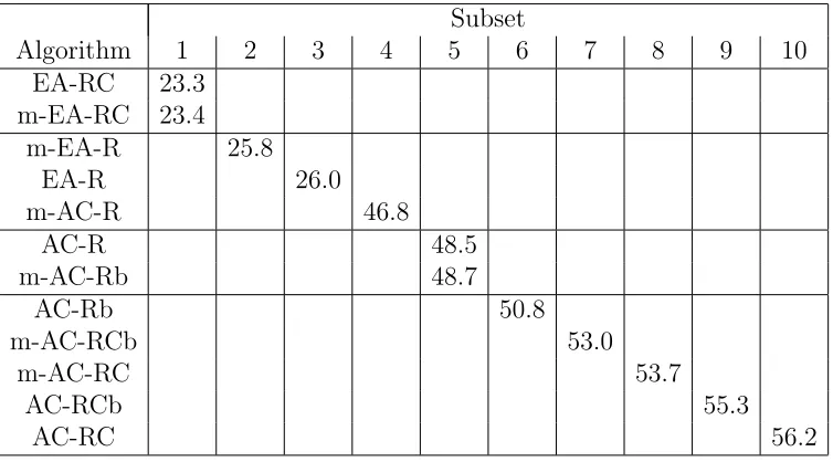
Table 2 shows the statistically significantly different sub-groups with their mean values for all problems. The following observations can be made:
• The use of an EA as the global search component of search means runs of the search process discover lower cost solutions than using ACO.
• In every case except EA-RC (where the difference is not significant), the addition of local search enables discovery of lower cost solutions.
• Redundancy avoidance helps the EA.
Estimated Marginal Means 60 40 20 0 Algorithm m-AC-RCb AC-RCb m-AC-RC AC-RC m-AC-Rb AC-Rb m-AC-R AC-R m-EA-RC EA-RC m-EA-R EA-R SC15 SC14 SC13 SC12 SC11 SC10 SC09 SC08 SC07 SC06 SC05 GDP CBS Problem Algorithm m-AC-RCb AC-RCb m-AC-RC AC-RC m-AC-Rb AC-Rb m-AC-R AC-R m-EA-RC EA-RC m-EA-R EA-R Min Fmin 60 40 20 0 SC15 SC14 SC13 SC12 SC11 SC10 SC09 SC08 SC07 SC06 SC05 GDP CBS Problem
Figure 2: Overall (bottom) and Mean (top) of best solution found for each problem.
5.3. Effect of Problem Characteristics
Table 2: Results of testing to discriminate homogenous subsets. Values in cells are means for lowest cost found per run.
Subset
Algorithm 1 2 3 4 5 6 7 8 9 10
EA-RC 23.3 m-EA-RC 23.4
m-EA-R 25.8
EA-R 26.0
m-AC-R 46.8
AC-R 48.5
m-AC-Rb 48.7
AC-Rb 50.8
m-AC-RCb 53.0
m-AC-RC 53.7
AC-RCb 55.3
AC-RC 56.2
found. For each of these local optima was stored its cost, the difference in cost, and the number of different values (i.e., the extension of Hamming Distance) from the lowest cost solution found during the 100,000 runs.
Table 3 displays the lowest cost solutions found, with the hand-crafted results for comparison. Immediately noticeable is that despite the variation in mean search results noted above, the best solution found for each problem does not change to anything like the same extent. To put this another way, it would appear that neither the scale nor complexity of the problem greatly affect the cost of the global optimum, but they do make the landscape harder to search. This is equally true for both encodings, which of course have differ-ent genotype-phenotype mappings, and hence presdiffer-ent differdiffer-ent landscapes to the global search element. We note that in every case meta-heuristic search was able to find solutions better than the provided hand-crafted solutions, and inspection showed that these made semantic sense.
Table 3: Lowest Cost solutions found by different search algorithms for each problem.
Enco Search Problem
ding Method CBS GDP SC5 SC7 SC9 SC11 SC13 SC15 Perm. mAC-R 9.2 30.3 42.5 49.4 48.0 41.5 41.5 42.5
mEA-R 16.3 19.9 21.5 24.7 25.7 25.9 26.5 25.8 LS 16.9 20.4 21.6 26.5 25.7 28.1 27.8 27.2 Int. mEA-RC 14.9 18.3 19.0 21.9 22.4 23.5 24.4 24. 6
LS 16.3 19.8 20.9 22.7 24.1 24.7 25.1 25.2
Human 14.6 36.5 34.3
Best 9.2 18.3 19.0 20.5 22.4 20.6 20.6 21.6
problem. The top pane of Figure 3 shows for each problem the distribution of the normalised fitness differences - that is to say, of (fcomb−fcomb∗ )/fcomb∗ .
As can be seen, the local optima in the permutation-based landscapes have higher costs (larger normalised differences) than their counterparts in the integer-encoded redundancy-avoiding landscapes. In both cases there is a very wide spread of values, and given that the median normalised difference is mostly over 0.5, most of the local optima have costs more than 150% of the global best. Apart from the CBS results, it is also noticeable that the distributions of values are fairly constant for the integer encodings. However for the permutation encodings they rise from GDP through to SC5 and SC7 (where most local optima costs are twice the global best) before reducing as the number of classes increases. These findings are line with the results of the algorithm comparison above, especially for ACO, and suggest a reason for those results - that ACO is getting stuck in local optima, and that these tend to have higher fitness values for some problems.
The bottom pane of Figure 3 shows the normalised distance - that is, proportion of elements with a different class label to that in the estimated global optimum. This shows that typically local optima have no elements with values in common to the estimated global optimum for permutation encodings. For the redundancy-avoiding integer encoding, it is noticeable that CBS,GDP and SC5, which all have 5 classes, have similar distributions, and that the typical distance rises thereafter for the SC problems.
Problem SC15 SC13 SC11 SC09 SC07 SC05 GDP CBS
Normalised Fitness Difference
3.00 2.50 2.00 1.50 1.00 .50 .00 Permutation Integer (C) Representation Problem SC15 SC13 SC11 SC09 SC07 SC05 GDP CBS
Normalised Distance to global optimum
[image:22.612.118.502.123.383.2]1.00 .90 .80 .70 .60 .50 Permutation Integer (C) Representation
Figure 3: Box plots of normalised fitness difference between (top), and distance to (bottom) local and global optimum. Boxes indicate interquartile range, line is median. Circles denote outliers more than 1.5 and 3 box-widths from quartiles and asterisks more than 3.
Normalised Fitness Difference
2.5 2.0 1.5 1.0 .5 .0 Problem SC15 SC13 SC11 SC09 SC07 SC05 GDP CBS NormalisedD(x,best) 1.0 .5 .0 2.5 2.0 1.5 1.0 .5 .0 1.0 .5
.0 .0 .5 1.0.0 .5 1.0.0 .5 1.0.0 .5 1.0.0 .5 1.0.0 .5 1.0
Representation
Permutation
Integer (C)
[image:22.612.120.498.463.578.2]difference vs normalised distance, with regression lines fitted. Although the co-efficient of correlation is fairly low, it is worth noting the slope of the lines. These provide clues to the reason for worse performance observed for ACO and local search on GDP, SC5 and SC7 on the permutation landscapes: there is a negative correlation between cost difference and distance. In other words the more highly fit local optima tend to be further from the global optimum. In contrast, for the SC11,SC13 and SC15 problems the correlation is positive, and so moving from one local optimum to a better one will, on average, lead towards the global optimum.
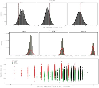
To examine how much of this was the effect of the redundancy in the encoding, we re-ran the local search experiments for the 5-class problems with integer encoding. At the end of each experiment we generated all 5! = 120 possible versions of the best solution by permutating the class labels. Then for each local optima we recorded the distance to the closest copy of the global optimum. Again, measuring the excess cost, and normalised distance, we examined the spread of these measures as shown in Figure 5. As can be seen from the top two panes, the distributions of distances and excess cost follow a normal distribution in all three problems. Comparing excess cost to the pooled mean and median values, the CBS distribution contains more high cost solutions and the GDP fewer. Comparing the distances, it is noticeable that the spread of values is far wider, and the mean of the distribution lower, for the CBS than the GDP, which in turn is wider than the SC. This is clear from the scatter plot as well. Since there are more local optima closer to the global optimum for CBS, it follows that there is a higher chance of escaping from an arbitrary local optimum (e.g., reached early in randomly initialised search) to a global optimum on that problem.
The next aspect to be considered is the effects of scale and complexity. Table 4 shows the co-efficient of determination R2, a measure of the amount
of the observed variation explained by a linear regression model of the cost of the solutions found in terms of different problem descriptors. The rows give the results from the 100,000 iterations of local search on two different representations, and from the meta-heuristic search algorithms (100 runs per algorithm variant). Scatter plots showed that in every case the correlation was weakly positive - the cost of the local optima found increased in line with the different measures of problem scale or complexity.
Percentage Excess Cost 100 80 60 40 20 0 Frequency 6,000 5,000 4,000 3,000 2,000 1,000 0 100 80 60 40 20
0 0 20 40 60 80 100
Problem
SC05 GDP
CBS
Percent distance from global optimum 80.00 60.00 40.00 20.00 .00 Frequency 30,000 20,000 10,000 0 80.00 60.00 40.00 20.00
.00 .00 20.00 40.00 60.00 80.00
Problem
SC05 GDP
CBS
Percent distance from global optimum
80 70
60 50
40
Percentage Excess Cost
[image:24.612.117.501.129.470.2]100 80 60 40 20 0 SC05 GDP CBS Problem
Figure 5: Histograms of excess cost (Top), and distance to closest copy of global optimum (Middle), and Scatter plots (Bottom) showing the distribution of local optima for the five class problems. Reference lines show the mean and median of the pooled distributions
• For all algorithms the number of uses per method is insignificant.
• All other effects appear significant, but since they only have three values they are effectively serving as proxies for the problem instance.
• The degree of correlation is insignificant (R2 < 0.15) for the other possible predictors “uses/methods/attributes per class”.
Table 4: Co-efficients of determination for linear models relating various measures of problem characteristics to the observed quality of solutions.
Best vs.
R2 Classes Attributes Methods Uses Uses per Uses per method attribute LS int. 0.155 0.529 0.487 0.398 0.025 0.378 LS perm. 0.005 0.477 0.294 0.461 0.006 0.175 EA int. 0.673 0.692 0.615 0.547 0.031 0.471 EA perm 0.489 0.816 0.723 0.644 0.003 0.559 AC perm. 0.148 0.836 0.544 0.805 0.034 0.358
procedure converts continuous variables into ordinal ones, then uses forward stepwise predictor selection based on information criteria to build a model based on this series of binary decisions (e.g.,“classes= 5”, “classes= 6”, etc.). Therefore the choice of effects selected, and their relative importance, gives insight into the factors that affect the quality of results found.
For the results of EA-RC/m-EA-RC the model produced yielded a pre-dictive accuracy of 96.6%. The relative importance of classes was 0.746, that of the transformed variable “attributes=16” was 0.254, all other effects were removed by modelling process as insignificant.
By way of contrast, repeating this process for the pooled results with the permutation representation only yielded a model with a 44.5% predictive accuracy. The importance of the transformed value of Uses per Attribute was 0.915, that of classes was 0.085, all others were removed. If the tool was allowed to use the type of global search component, the predictive accuracy increased to 88.2%. The relative importance of effects selected in the model was global search (0.701), attributes 0.278 and classes 0.014.
6. Analysis
in the presence of many local optima. To give an idea of the number of these, there were less than ten duplicates in the 100,000 local optima located per problem. Moreover, the local optima appear to become both higher cost, and on average further from the global optimum as the complexity of the problem is increased.
Taken together with the results for search performance, Figure 5 shows a clear relationship between the distribution of local optima within the search space, and the ability of search algorithms to reliably locate solutions close to the estimated global minimum cost.
For all but the simplest problem (CBS), EA-based variants outperformed their ACO-based counterparts, and behaved robustly with respect to problem scale and complexity. The two ways of adding of problem-specific knowledge to the EA (reducing redundancy via the choice of encoding, and using a repair function) were both beneficial, as was the use of instance-specific information in the local-search algorithm.
In contrast, although the ACO required the repair function for the more complex functions, adding information via distance heuristic, and reducing redundancy were both detrimental to the ACO-based variants. We hypoth-esize that both of these may have the effect of focussing search, causing premature convergence. To test this, we examined ACO runtime logs, which revealed that the lowest cost solutions are typically discovered an order of magnitude sooner than the equivalent EA-based experiments. This suggests that basins of attraction of fewer local optima are sampled during search. Given the relationship between the quality of local optima and their distance from the global optima (and hence from other low cost solutions) shown in Fig. 4 this explains the performance curves seen in Fig. 2. For some mid-scale problems (SC5-7) the negative quality-distance correlation means that algo-rithms which move from local optima to local optima will actually move away from the global optima, and because of the redundancy of the permutation encoding will actually be moving into more sparsely populated regions, where they are more likely to to become trapped. There remains the possibility that our results would dramatically change if we could find some “magic” set of settings that reduced this problem of ACO premature convergence, since we did not exhaustively tune the parameter values. However, our preliminary investigations did include all combinations of several different values for each parameter, in addition to the recommended settings.
our choice of fitness function.
It should be noted at the outset that the field suffers from a lack of bench-marks. Our previous papers use three problems, the other papers cited in Section 2.2 use only one [2, 27]; or two [15]. Clearly this poses a threat to the validity of those results, and our findings above. The development of a reli-able benchmark set would greatly aid comparison of experimental methods. Elsewhere we have reported on the design of tuneable randomised test land-scape generators where various factors such as the problem size, the number and relative size of local optima, the degree of epistatic interference between partitions of the search space, and “deceptiveness” could be tuned to facili-tate algorithm design and analysis [23]. Hence some of our experimentation into the factors that appear to make problems hard for SBSE. It would ap-pear that, although the quality of the best solution present does not change much for our weighted-sum metric, the problem size (effectively the size of the graph to be partitioned), and the number of uses per attribute (closely related to the degree of the graph) are the major factors in determining the reliability with which the lowest cost solutions can be found.
The question of the cost metric used is more subtle. In earlier papers we reported results from fCBO on its own, as well as in combination withfN AC,
7. Conclusions
We preface our remarks by the acknowledging that the lack of bench-marks, especially large-scale instances for this task mean that we must be somewhat cautious in our findings. Nevertheless, our results have gone some way towards identifying the problem characteristics that are important to vary when selecting or constructing a range of test instances.
For early lifecycle design of object-oriented class models, and given the computational budget allowed, using Evolutionary Algorithms as the global search component of an algorithm outperforms the use of Ant Colony Opti-misation. EAs are more capable at handling constraints, and the influence of different search components such as repair functions, redundancy avoidance and local search is beneficial to the search process. Although competent on the less complex problems, using ACO on the more complex solutions often failed to find valid solutions without the use of a repair function. Other methods for incorporating problem-specific information appeared to exacer-bate the tendency of the ACO to prematurely converge. On certain problems this causes a rapid decrease in performance, and landscape analysis revealed that this coincided with a landscape structure exhibiting a positive fitness-distance correlation, where low-cost local optima are more typically further from the global optimum than higher cost ones.
To better understand the search landscapes, and how these related to problem characteristics, we used iterated random-restart local search to probe the local optimum structure of the landscape. All problems contained a huge number of local optima, with little structure to their distribution relative to the estimated global optimum. Both increasing complexity (classes) and scale (number of problem elements to be grouped) caused the cost of local optima to increase. Interestingly, however, there was not a corresponding change in the cost of the best solution ever found, which we use as a proxy for the global optimum.
References
[1] C-E. Bichot and P. Siarry. Graph Partitioning: Optimisation and Ap-plications. ISTE Wiley. 2011.
[2] M. Bowman, L. C. Briand, and Y. Labiche. Solving the Class Respon-sibility Assignment Problem in Object-Oriented Analysis with Multi-Objective Genetic Algorithms. IEEE Transactions on Software Engi-neering, 36(6):817–837, Nov. 2010.
[3] W. Brown, R. Malveau, H. McCormick, and T. Mowbray.Anti-Patterns: Refactoring Software, Architectures, and Projects in Crisis. Wiley, 1998.
[4] B. Curtis, H. Krasner, and N. Iscoe. A Field Study of the Software Design Process for Large Teams. Communications of the ACM, 31(11), 1268-1287. 1998.
[5] A. E. Eiben and J. E. Smith. Introduction to Evolutionary Computing. Springer: Heidelberg, Berlin, New York, 2003.
[6] E. Falkenauer. Genetic Algorithms and Grouping Problems Wiley. 1998.
[7] R.L. Glass. Facts and Fallacies of Software Engineering. Addison-Wesley. 2003.
[8] Graph Partitioning Archive.
http://staffweb.cms.gre.ac.uk/wc06/partition/ accessed November 2013.
[9] N. Krasnogor and J. Smith. Competent memetic algorithms: model, taxonomy and design issues. IEEE Transactions on Evolutionary Com-putation, 9:474–488, 2005.
[10] C. Larman. Applying UML and Patterns: An Introduction to Object-Oriented Analysis and Design and Iterative Development, 3rd Ed. Dor-ling Kindersley Pvt Ltd. 2008.
[11] R. Lewis and E. Pullin. Revisiting the Restricted Growth Function Genetic Algorithm for Grouping Problems Evolutionary Computation
[12] S. Meyer-Nieberg and H.-G. Beyer. Self-adaptation in evolutionary al-gorithms. In F. G. Lobo, C. F. Lima, and Z. Michalewicz, editors, Pa-rameter Setting in Evolutionary Algorithms, pp. 47–75. Springer, 2007.
[13] M. Petre. Insights from Expert Software Design Practice. In Proc. Joint 12th European Software Engineering Conf. and 17th ACM SIGSOFT Symp. on the Foundations of Software Engineering, pp 233-241. 2009.
[14] M. Serpell and J. Smith. Self-Adaption of Mutation Operator and Prob-ability for Permutation Representations in Genetic Algorithms. Evolu-tionary Computation, 18(3):1–24, Feb. 2010.
[15] O. Sievi-Korte, E. M¨akinen, and T. Poranen. Simulated Annealing for Aiding Genetic Algorithm in Software Architecture Synthesis. Acta Cy-bernetica 21:2,235-265, 2013.
[16] C. Simons. Case study specifications, available at http://www.cems.uwe.ac.uk/˜clsimons/casestudies.
[17] C. Simons and I. Parmee. Elegant object-oriented software design via interactive, evolutionary computation. IEEE Transactions on Systems, Man, and Cybernetics, Part C, 42(6):1797–1805, 2012.
[18] C. Simons, I. Parmee, and R. Gwynllyw. Interactive, Evolutionary Search in Upstream Object-Oriented Class Design. IEEE Transactions on Software Engineering, 36(6):798–816, 2010.
[19] C. Simons and J. Smith. A Comparison of Evolutionary Algorithms and Ant Colony Optimization for Interactive Software Design. InProceedings of the 4th Symposium on Search Based-Software Engineering, p.37, 2012.
[20] C. L. Simons and J. E. Smith. A Comparison of Meta-heuristic Search for Interactive Software Design.Soft Computing17(11):2147–2162, 2013.
[21] C.L. Simons, J. Smith and P. White. Interactive ant colony optimization (iACO) for early lifecycle software design. Swarm Intelligence, 8(2):139-157, 2014.
[23] R.E. Smith and J.E. Smith New Methods for Tuneable, Random Land-scapes. Foundations of Genetic Algorithms, pp. 47–67. Morgan Kauf-mann. 2001.
[24] T. Stuetzle. ACOTSP, version 1.2, available at http://www.aco-metaheuristic.org/aco-code.
[25] T. Stuetzle and H. H. Hoos. Max-min ant system. Future Generation Computer Systems, 16(8):889–914, 2000.
[26] D. Svetinovic, D.M. Berry, and M. Godfrey. Concept identification in object-oriented domain analysis: why some students just don’t get it. In Proceedings of the International Conference on Requirements Engi-neering, 189-198. IEEE Computer Society, 2005.
[27] S. Vathsavayi, H. Hadaytullah, and K. Koskimies. Interleaving human and search-based software architecture design. Proceedings of the Esto-nian Academy of Sciences, 62(1):16, 2013.
[28] G. Wang. Ant Colony Metaheuristics for Fundamental Architectural Design Problems. PhD Thesis, Uni. California in Santa Barbara, 2007.
[29] R. Wirfs-Brock, and A. McKean. Object Design: Roles, Responsibilities, and Collaborations. Addison-Wesley. 2003.