Cost Efficiency in UK and
Irish Credit Institutions
TREVOR FITZPATRICK* European Central Bank
KIERAN MCQUINN**
Central Bank and Financial Services Authority of Ireland
Abstract: This paper presents aggregated cost efficiency scores for a balanced panel of British and Irish credit institutions and relates these scores to loan loss reserves as a first step in investigating their usefulness as possible indicators of financial fragility. The efficiency scores are obtained using the two most popular methods of efficiency measurement – data envelopment analysis (DEA) and the stochastic frontiers approach.
I INTRODUCTION
C
entral bankers have traditionally endeavoured to better understand the roles that financial intermediaries and especially credit institutions play in the transmission mechanism of monetary policy. One aspect of this work involves the monitoring of forces such as deregulation, financial innovation, the impact of information technology and competition on the banking sector. An increasingly popular way of assessing the impact of these latent factors is to empirically identify cost efficiencies/inefficiencies of credit institutions.45
* E-mail: trevor.fitzpatrick@ecb.int
A second associated concern of central banks relates to financial stability, i.e., the absence of systemic crisis within the financial sector. An efficient and well-functioning financial system is a prerequisite to maintaining a stable financial environment. Given that credit institutions constitute a sizeable component of any particular financial system, the development of a robust set of efficiency measures may serve as an important input into indicators of banking fragility.
This paper seeks to address these two issues simultaneously by first generating a series of cost efficiency scores for a balanced panel data set (1996-2001) of 30 UK and Irish credit institutions with both parametric and non-parametric techniques. Subsequentially, these scores are used as explanatory variables in a second series of regressions, where the dependent variable is an indicator of the loan loss reserve of a particular credit institution. As such, the paper seeks to complement a comparatively new area of the banking efficiency literature, which explores the relationship between both the efficiency and the asset quality of a bank. To date, this work has mainly concentrated on US banks (see Berger and DeYoung (1997) for example). Therefore, our contribution is to extend this analysis to the UK and Irish banking sector in the context of both parametric and non-parametric efficiency scores. It should be thought of as a preliminary look at possible ex anteindicators of individual bank fragility and as a crosscheck on the efficiency scores.
In stressing the importance of bank level measurements of efficiency to policy makers in particular, Bauer et al. (1998) advance a set of consistency conditions, which they believe, efficiency measures from different approaches should meet in order to be of ‘optimal use’. One of these conditions is that measured efficiencies, irrespective of the computational technique adopted, should be reasonably consistent with standard nonfrontier performance measures. Consequently, the objectives of an ex-post evaluation are twofold. First, the establishment of a relationship with non-frontier banking indicators provides a certain validation of the efficiency scores achieved and a potential ranking mechanism between alternative scores where significant differences occur between parametric and non-parametric methods of estimation/ calculation. Simultaneously, however, the establishment of a relationship between efficiency scores and these indicators is significant, in itself, as useful information concerning the underlying performance of financial institutions can be inferred from these scores or models using these scores.
in each country. A summary of the credit institutions included in the data set is presented in Table 1.
Table 1: List of Credit Institutions Used in Sample (1996-2001)
Barclays Bank PLC Cheshire Building Society
Royal Bank of Scotland Principality Building Society
Alliance and Leicester Newcastle Building Society
Northern Rock PLC Norwich and Peterborough Building Society
Bradford and Bingley PLC Scarborough Building Society
Britannia Building Society Bank of Scotland
Yorkshire Bank PLC Halifax PLC
Yorkshire Building Society *Bank of Ireland
Portman Building Society *Allied Irish Bank PLC
Clydesdale Bank PLC *Anglo-Irish Bank PLC
Co-Operative Bank PLC *EBS Building Society
Leeds and Holbeck Building Society *First Active PLC
West Bromwich Building Society *Irish Nationwide Building Society
Northern Bank Limited *ACC Bank PLC
Derbyshire Building Society *National Irish Bank Limited
Note:*denotes an Irish credit institution.
The rest of the paper is laid out as follows: Section II introduces both parametric and non-parametric methods of efficiency measurement. Data and results of the initial empirical analysis are discussed in Section III, while Section IV reports the results of the ex-post empirical evaluation of the efficiency scores. Section V offers some concluding comments.
II COST EFFICIENCY ESTIMATES
In this section we present two of the most popular means of generating efficiency scores. We adopt the popular ‘frontier’ approach, where the efficiency of a bank is gauged relative to a frontier of best practice. In particular, we use both the parametric stochastic frontier model and the non-parametric data envelopment analysis (DEA) approaches to generate efficiency scores.
(TE), most parametric cost function applications assume full allocative efficiency resulting in CE being closely related to TE.1From the parametric
perspective, we specify the following cost function for the sample of Irish and British credit institutions.
Ci= f(Yi*, Pi, α) e(κi+ξi) (1)
where
Ci = bank level costs of production, Yi* = optimum bank level outputs, Pi = prices of bank level inputs Xi, f() = represents the cost function,
α = vector of parameters to be estimated,
κ = independent and identically distributed errors i.e., κi∼ N(0, σκ2) and ξi = non-negative random variables which are assumed to account for the
cost of inefficiency in production. These are usually assumed to be ∼ N|(0, σξ2)|. ξi measures how far the individual bank operates above
the cost function. The cost function measure of technical efficiency is defined in the following manner
CE = E(Ci|ξi, Pi) / E(Ci|ξi= 0, Xi) (2)
CE has a value of between one and infinity. (2) can be shown to be equivalent to2
CE = exp (ξi) (3)
The unobservable ξi is obtained by deriving expressions of the conditional expectation of ξi, conditional on the observed value of (κi + ξi). These expressions can be derived from equivalent expressions for the case of production function inefficiency measurements outlined in Battese and Coelli (1992) and Battese and Coelli (1993).
A specific functional form is assumed for the cost function specified in (1). Following other applications (Vander-Vennet (2002) and Bikker (2002) for example) we employ the translog cost function.3This is given by the following4
1For a full discussion of this point see Chapter 9 of Coelli et al. (1998). 2The exponent is taken as the translogcost function is specified.
3Standard likelihood ratio tests are performed to test the suitability of the more restrictive
Cobb-Douglas functional form nested within the translog.
4Note that in the estimation we impose symmetry on the cross-products i.e.
2 5
1 2 2
ln Ci= α0+ αj ln Yj + αj ln Pj + –
αjk ln Yj ln Yk
j=1 j=3 2 j=1 k=1
1 5 5 2 5 (4) + –
αjk ln Pj ln Pk+
αjk ln Yj ln Pk+ κi + ξi
2j=3 k=3 j=1 k=3
The cost inefficiency model outlined in (1) and (4) estimates a static level of inefficiency for each bank for the specified time period. However, the availability of a panel data set enables the estimation of a time-varying model of inefficiency where inefficiency levels may increase or decrease through time. Battese and Coelli (1992) have modified (4) to allow for dynamic estimates of inefficiency
2 5
1 2 2
ln Cit= α0+ αj ln Yjt + αj ln Pjt + –
αjk ln Yjt ln Ykt
j=1 j=3 2 j=1 k=1
1 5 5 2 5 (5) + –
αjk ln Pjt ln Pkt+
αjk ln Yjt ln Pkt+ κit + ξit
2j=3 k=3 j=1 k=3
where the efficiency estimate ξit in (5) is now equal to ξiexp [–φ(t – T)] – commonly referred to as the time-varying decay model.5 The ξi’s are now
assumed to be i.i.d. as a generalised truncated-normal random variable of the N(µ, σξ2) distribution, t refers to the time period (t=1,…,T) and φ is an
unknown parameter, which is estimated. The parameterisation of Battese and Corra (1977) is employed, where σκ2and σξ2are replaced by σ2=σκ2+σξ2and γ=σξ2/(σκ2+σξ2). The parameter γmust lie between 0 and 1. The resulting
log-likelihood function, expressed in terms of these variance parameters, can be observed in the appendix of Battese and Coelli (1992).
In the last period of the panel, the exponential function, ξi exp [–φ(t – T)] has a value of 1, (t=T), so ξit=ξi. Therefore, if the parameter φ is positive, then –φ(t – T) φ(T – t) = non-negative and exp [–φ(t – T)]is ≥1. As a result, ξit ≥ ξi, thereby indicating a decreasing level of inefficiency over time. Conversely, a negative value of φ results in exp [–φ(t – T)] ≤ 0 and ξit ≤ ξi with levels of inefficiency now growing over time.6As this specification restricts inefficiency
5Inefficiency levels either decay towards or increase to a base level.
6Note that a particular feature of the inefficiency model outlined in (5) is that the cost inefficiency
effects of different credit institutions in a given year t is equal to an exponential function exp [–φ(t – T)] exp [–φ(T – t)] of the corresponding institution-specific inefficiency effects for the last year of the panel (the ξi’s). Therefore, this particular specification restricts the cost
movements across all credit institutions to move in a common direction for the time period, we also apply the time-invariant inefficiency model where φ is set equal to zero (i.e. (5) reduces to a panel application of (4)). This restriction is explicitly tested for in (5) above.
The second popular method of generating bank efficiency scores vis-à-vis frontiers of best practice is through non-parametric linear programming techniques. Non-parametric frontiers are constructed by envelopinga sample of individual units (credit institutions) with a frontier constructed by the credit institutions of best practice within the sample. Frain (1990) presents a neat exposition on the use of such techniques. Comprehensive reviews of the approach are also contained in Lovell (1993), Charnes et al. (1995) and Seiford (1996) while Coelli et. al. (1998) present an overview of the different programming options available.7
Under DEA, a non-parametric envelopment frontier over the data points is constructed with all observed data points residing on or above the cost frontier. Adopting the cost minimisation behavioural postulate enables the derivation of both estimates of cost efficiency and allocative efficiency (the quantity of inputs to produce a given level of outputs at minimum cost). For a cost minimising bank, under variable returns to scale, cost efficiency is obtained by solving the following minimisation problem for each bank, i = 1,2,…,S in each year of the sample
Minλ,xi*pi'xi*
subject to: Yλ ≥yi Xλ ≤xi*
N1' λ= 1
λ≥ 0 (6)
where λis a N * 1 vector of constants. Yis an N * S output matrix and Xis an M * S input matrix, with yi and xi being the corresponding N * 1 and M * 1 vectors of the ith bank. pi8is an N * 1 vector of bank input prices and xi* is the cost-minimising vector of input quantities for the ith bank given factor input prices piand output level yi. In this case, the cost efficiency (CE) of each bank in the sample is obtained via the ratio of minimum cost to actual, observed cost
CE = pi'xi* / pi'xi (7)
7In a recent contribution Wheelock and Wilson (2003), following work by Cazals et al.(2002),
adopt the non-parametric order-mfrontier, which measures the performance of credit institutions relative to expectedmaximum output among minstitutions using no more of each input than the given institution.
with a score of 1 indicating a point on the frontier and hence a perfectly cost efficient bank. This estimate of cost efficiency can then be checked against the estimate obtained under the stochastic cost function approach in (3).
III DATA AND EMPIRICAL RESULTS
Studies of the efficiency of the UK banking sector have been relatively scarce. Drake (2001), for instance, comments that ‘‘to date, however, no such analysis has been conducted for the UK banking sector as a whole’’. Using DEA, Drake (2001) generates efficiency scores for 9 UK credit institutions over the sample period 1984-1995. Drake and Simper (2003) provide a breakdown of efficiency scores into pure technical, scale and overall efficiency for 20 UK credit institutions over the 1995-2001 period. Their scores are also derived from non-parametric techniques. To our knowledge, no study, to date, presents parametrically generated cost efficiency scores for UK credit institutions (unless within a broader sample of the euro wide area) and, certainly, no study compares parametric and non-parametric scores for the UK financial system. In an Irish context, there also has been relatively few empirical investigations of bank level performance. McKillop and Glass (1991) looked at the internal workings of Allied Irish Bank from 1972 to 1988 while Glass and McKillop (1992) examined the performance within Bank of Ireland between 1972 and 1990. In both cases, scale and scope economies were explicitly examined. Lucey (1993) generated efficiency estimates for 17 Irish credit institutions over the 1988-1991 time period. The results suggest that Irish credit institutions over the period displayed a severe degree of inefficiency and that a level of inefficiency equal to a considerable portion of actual profits was lost due to various inefficiencies. However, as Lucey (1993) concedes, the results are significantly conditioned by the relative lack of information on individual credit institutions and the short time period involved in the empirical investigation.
banks. The data were checked to ensure that any institutions with implausible (i.e., total loans greater than total assets) or missing values were excluded. Consolidation and ownership issues (UK of Irish and vice versa) necessarily limits the number of credit institutions that we could include in our sample and we also exclude branches and subsidiaries of foreign credit institutions. This resulted in a balanced panel of 30 banks for 6 years.
In specifying the inputs and outputs of a bank for both parametric and parametric approaches, we follow the classification used in a non-exhaustive list of the more recent literature.9 In particular, we treat the
balance sheet level of total loans as a bank output (Yi). This involves the aggregation of commercial, consumer and other loans. Costs (C) consist of interest and non-interest expenses. Input prices are the price of labour (P3 = total personnel expenses/number of employees), the price of physical
capital (P4 = non-interest expenses – personnel expenses/corrected fixed
assets) and the price of financial capital (P5 = total interest expenses/
[image:8.498.77.434.370.507.2]total deposits). In ‘correcting’ the fixed assets figure, we follow the approaches of both Resti (1997) and Bikker (2002) in order to minimise the influence of so-called ‘book-keeping tricks’ on credit institutions’ reported fixed asset levels.10
Table 2: Summary of Cost and Output Data Used in Empirical Analysis: 1996-2001
Variable Notation Mean Std. Deviation
Costs: C 0.061 0.010
Outputs:
Loans Y1 0.734 0.094
N.I. Income Y2 0.009 0.006
Prices:
Labour P3 32.129 9.641
Physical Capital P4 0.850 0.504
Financial Capital P5 0.054 0.014
Note:N.I. = non-interest. All variables are in ratio form, C, Y1, Y2are normalised by
total assets while P3, P4and P5are prices per unit.
9Examples include Berger and Mester (1997); Cummins and Weiss (1998); Vander-Vennet (2002);
Carbo et al. (2003); Bikker (2002) and Clark and Siems (2002). Additionally, Frain (1990) provides a summary of some of the pre-1990 literature.
10For fixed assets, we use the fitted values from a quadratic regression of fixed assets on total
In addition, we include total non-interest revenue as a bank output (Y2).
Non-interest income has become increasingly important for credit institutions. For instance, in some countries, (such as Finland11), non-interest income can
account for over 50 per cent of total operating income. Rogers (1998), in examining the non-traditional activities of US commercial banks, argues that the omission of such non-traditional banking activities from a bank’s behavioural postulate can result in an understating of measured efficiency scores.12To minimise the effects of potential large-scale differentials amongst
the credit institutions in the sample, we normalise all cost and output data by total assets. Table 2 presents a summary of all cost and output data used for the institutions in the sample.
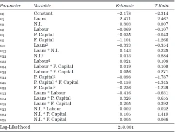
The parameter estimates of the time-varying decay translog cost function (6) are summarised in Table 3.13From the table it is evident that very few of
the parameter estimates are significant at even the 10 per cent level. In total, two of the 26 parameters of the cost function are significant at the 5 per cent level and only one additional parameter is significant at the 10 per cent level. Thus, a question arises as to the suitability of the translog in this particular application.14 It may well be, for instance, that the translog model is over parameterisedin this case.
Table 4 presents the results of the variance parameters associated with (6). Of particular interest in Table 4 are the results for the γand φparameters. Recall that γ must lie between 0 and 1. A score of 0.727 suggests that the majority of the total residual variation is due to the inefficiency effect i.e. a significant estimate of γmeans that the ξiexpression is warranted in the cost function and that a deterministic function, where credit institutions deviate from a frontier of best practice on the basis of random error alone, is not supported by the data.15The φparameter conveys information concerning any
movements in inefficiency levels for the time period in question. A significant and positive value for φdenotes a declininglevel of bank inefficiency for the period. While a positive estimate for φ is obtained, the parameter is not significant at the 10 per cent level. Thus, we are unable to conclude, with certainty, whether inefficiency levels for the sample of credit institutions have declined over the period. Table 4 also contains the results of a likelihood ratio
11Source:OECD Bank profitability data 2002.
12An additional reason for the inclusion of non-interest income as an output is to enable the
comparison of our results with similar type research.
13Estimates are obtained using the computer program FRONTIER Version 4.1, which is available
on the Centre for Efficiency and Productivity Analysis (CEPA) web-site at www.uq.edu.au/ economics/cepa/frontier.htm and Stata 8.0.
14Note the exact same model was estimated with Stata 8.0 for windows with similar parameter
estimates obtained. These results are available from the authors upon request.
Table 3:Translog Stochastic Cost Function Estimates
Parameter Variable Estimate T-Ratio
α0 Constant –2.178 –2.314
α1 Loans 2.471 2.467
α2 N.I. 0.303 0.807
α3 Labour –0.069 –0.107
α4 P. Capital –0.035 –0.043
α5 F. Capital –1.101 –1.266
α11 Loans2 –0.333 –0.354
α12 Loans * N.I. 0.143 0.225
α22 N.I.2 0.013 0.884
α33 Labour2 0.021 0.108
α34 Labour * P. Capital 0.019 0.109
α35 Labour * F. Capital 0.056 0.271
α44 P. Capital2 –0.098 –1.787
α45 P. Capital * F. Capital –0.158 –1.345
α55 F. Capital2 –0.236 –1.229
α13 Loans * Labour –0.416 –0.631
α14 Loans * P. Capital 0.326 0.655
α15 Loans * F. Capital 0.205 0.392
α23 N.I. * Labour 0.002 0.022
α24 N.I. * P. Capital 0.105 1.419
α25 N.I. * F. Capital 0.005 0.066
Log-Likelihood 259.001
Note: N = 180 i.e. 30 credit institutions and 6 time periods. N.I. refers to non-interest income, P. = physical and F. = financial.
Table 4: Hypothesis Test and Variance Parameter Translog Estimates
Variance Parameters Estimate T-Ratio
σ2 0.006 1.418
γ 0.727 1.959
µ 0.099 2.232
φ 0.074 1.476
Hypothesis Test τ Decision
H0: αii,i=1,…,5= 0 24.47 ?
Note: τ is a likelihood ratio statistic calculated as –2[log(likelihood(H0)) –
log(likelihood(H1))]. It has an approximate chi-squared distribution with degrees of
freedom equal to the number of independent constraints under the H0hypothesis. The
[image:10.498.75.436.452.555.2]test between the more restrictive Cobb-Douglas specification and that of the translog. At the 1 per cent level, we are unable to reject the null of the Cobb-Douglas, while at the 5 per cent level we obtain a test statistic of 24.47 versus a critical value of 25. Given this result and the relatively small number of significant parameters with the translog approach, we elect to estimate the same model with the Cobb-Douglas specification.
Both the parameter estimates of the cost function as well as the variance estimates associated with the Cobb-Douglas model are presented in Table 5. Nearly all parameter estimates are significant at the 1 per cent level. The variance parameters are somewhat reassuring, in that, all estimates are significant at the 1 per cent level and the estimates for γ and φ are quite similar to those achieved with the translog (T) approach i.e. (γ = 0.727 (T) versus 0.794 and φ = 0.074 (T) versus 0.048). Therefore, a stochastic specification is again supported by the data,16 while the significance of the
[image:11.498.70.427.317.487.2]parameter suggests that inefficiency is declining across the sample for all credit institutions.17
Table 5: Cobb-Douglas Stochastic Cost Function Estimates
Parameter Variable Estimate T-Ratio
α0 Constant –1.227 –9.240
α1 Loans 0.0581 1.749
α2 N.I. 0.041 3.096
α3 Labour 0.062 2.038
α4 P. Capital 0.179 7.783
α5 F. Capital 0.584 21.737
Log-Likelihood 246.763
Variance Parameters
σ2 0.010 3.345
γ 0.791 14.218
µ 0.182 4.325
φ 0.048 3.714
Note: N = 180 i.e. 30 credit institutions and 6 time-periods.
Table 6, presents a statistical summary of cost inefficiency scores under both parametric and non-parametric approaches. We present results for both parametric approaches and for the DEA model. Results are presented by splitting the sample of credit institutions into either a ‘big’ or ‘small’ category.
16The null hypothesis of a one-sided error is again rejected with a likelihood ratio test.
17However, we also estimate the time-invariantpanel model (φ = 0) for both the translog and
This is determined by the average value of a bank’s total assets over the sample period. One significant difference in the estimation/calculation of the inefficiency scores should be noted at this point. Stochastic estimates of bank scores are obtained from a panel data set for 1996-2001, whereas scores under the programming approach are achieved on a multi-annual basis i.e. scores are determined for relevant credit institutions for 1996, thenfor 1997 etc. up until 2001. Programming scores in 2001, for example, are not affected by bank scores in, say, 1998.
[image:12.498.76.432.228.475.2]In general, all approaches reveal cost inefficiencies in the sample of UK and Irish credit institutions. Depending on the method used, the average degree of inefficiency can be as great as 22 per cent (Cobb-Douglas) or 17 per cent for both the translog and DEA method. Contrasting the scores from both parametric approaches first, it would appear that the degree of inefficiency is greater under the Cobb-Douglas approach with big credit institutions, in Table 6: Parametric and Non-Parametric Cost Inefficiency Estimates
(Time-varying Decay): Statistical Summary
Cobb-Douglas Big Small Irish UK
Average 0.162 0.216 0.223 0.177
Range 0.33 0.158
St. Deviation 0.098 0.036
Skewness 0.859 –1.320
C. of Variation* 0.601 0.167
N 90 90 8 22
Translog
Average 0.089 0.174 0.188 0.111
Range 0.254 0.187
St. Deviation 0.085 0.050
Skewness 1.289 -0.454
C. of Variation* 0.96 0.288
N 90 90 8 22
DEA
Average 0.095 0.169 0.190 0.116
Range 0.241 0.299
St. Deviation 0.093 0.076
Skewness 0.419 -0.523
C. of Variation* 0.973 0.451
N 90 90 8 22
particular, being over 7 per cent more efficient with the translog approach. However, the translog scores would appear to be more volatile as suggested by the coefficient of variation. Both sets of results suggest that larger credit institutions, are the more efficient. As such, the finding tallies with those of Eisenbeis et al.(1999) for US banks who find that, on average, smaller banks tend to deviate more than larger banks from their respective cost frontiers. Furthermore, in an evaluation of the performance of UK banks, Drake (2001) found tentative evidence to suggest that very large UK banks were less inefficient than their smaller competitors. Using a similar timeframe as the present study, Drake and Simper (2003) estimate that overall efficiency for UK retail banks increased from 85 per cent in 1995 to 90 per cent in 2001.
Both parametric approaches suggest that UK credit institutions are more efficient than their Irish counterparts. The relative difference in inefficiency is greater, however, for the translog approach at approximately 7 per cent. This contrasts with a difference of 4 per cent between both sets of credit institutions under the Cobb Douglas approach. We empirically test the apparent differences in the mean efficiency scores (i) between big and small credit institutions and (ii) between UK and Irish credit institutions. A t-test of no significant difference between the two sets of mean efficiency levels is rejected for all models at the 1 per cent level.18
In order to further explore some of the results from the econometric application, we conduct some additional estimation. In particular, we explicitly examine the relative cost structure of both Irish and larger credit institutions relative to the general sample. This is motivated by the clear differential in average efficiency scores between Irish and UK credit institutions and the apparent greater efficiency of larger credit institutions. Accordingly, the Cobb-Douglas model is re-estimated with two dummies included for Irish credit institutions (D1) and for the ‘big’ credit institution
category (D2). The results are presented in Table 7. On average, Irish credit
institutions would appear to have statistically significantly higher costs relative to their UK counterparts, while larger credit institutions, as suggested by their efficiency scores, have a significantly lower cost base.19
The results for the non-parametric scores are quite similar in magnitude to those of the parametric applications, in particular, the translog model. This contrasts with results from both Eisenbeis et al. (1999) and Berger and Humphrey (1997) who both found in comparisons of parametric and
non-18The test statistic tests for differences between the means of two groups Xand Ywhere the null
hypothesis is H0: µX =µY and σX2 and σY2 are unknown but σX2 ≠ σY2.
19We also estimate the time-invariantcost function for both parametric applications, however, we
parametric inefficiency scores for US banks, that non-parametric approaches yielded larger levels of inefficiency. Indeed, Eisenbeis et al. (1999) actually found that DEA inefficiency scores were over twice the level of the corresponding stochastic cost function estimates. The smaller non-parametric efficiency scores in our case, may be explained by the relatively smaller sample employed with the DEA averages being influenced by those credit institutions achieving efficiency scores of 1, that is, perfect cost efficiency. The average scores for UK and Irish credit institutions are remarkably similar to those of the translog approach with a 7 per cent difference in inefficiency between the two sets of credit institutions.
Based on our parameter estimates, we also examine the issue of scale economies within the sample of credit institutions. We follow Hughes et al. (2000) and explicitly measure scale economies by calculating the inverse of the cost elasticity of output
1
scale economies = ––––––––2 (8)
∂ln C
Σ
–––––– i=1∂ln Yi [image:14.498.76.435.111.304.2]where scale economies > 1 implies increasing returns to scale. Based on our Cobb-Douglas estimates, we obtain a value of 10.09. Thus, economies of scale Table 7: Cobb-Douglas Stochastic Cost Function Estimates with Dummies
Included
Parameter Variable Estimate T-Ratio
α0 Constant –1.052 –10.964
α1 Loans –0.086 –1.579
α2 N.I. 0.061 4.912
α3 Labour 0.054 2.169
α4 P. Capital 0.179 9.149
α5 F. Capital 0.579 22.680
α6 D1 0.053 3.489
α7 D2 –1.159 –6.384
Log-Likelihood 260.907
Variance Parameters
σ2 0.005 5.543
γ 0.579 9.308
µ 0.107 2.262
φ 0.084 2.225
Note:N = 180 i.e. 30 credit institutions and 6 time-periods. D1is the dummy for Irish
would appear to pertain within the sample. While we highlight this finding as a possible avenue for further exploration, the comments of Berger and Mester (1997), who found evidence of scale economies for a sample of US banks, are somewhat applicable in our case:
(1) First, scale economies may exist because of the relatively low interest rate environment of the sample (1996-2001). Given that ‘traditional’ intermediation is still the most important function of the institutions in our sample, it is unsurprising that interest expenses are the largest expense item. On average, these interest expenses are larger for big credit institutions than small credit institutions because a larger proportion of large credit institutions’ liabilities tend to be market-sensitive.
(2) Improvements in technology and applied finance may have cut costs more for larger credit institutions than smaller institutions. Improvements in Information Technology (IT) have reduced costs in back office (payments processing) and as well as at the retail end (i.e., credit scoring). This may have reduced the costs of extending loans, credit cards etc., more for larger credit institutions.
In conclusion, a comparison of the results under both the parametric and non-parametric methodologies reveals both differences and similarities, a conclusion also reached in an international survey of efficiency scores by Berger and Humphrey (1997). While the results from the translog model and the DEA approach are similar, the Cobb-Douglas functional form would appear to offer a better characterisation of the production technology of credit institutions in the sample. Furthermore, in comparisons with other work, the results from the Cobb-Douglas form and the DEA scores are quite similar. In the next section, we explore the informativeness of the inefficiency scores in terms of their potential relationships with nonfrontier indicators of banking performance.
IV EFFICIENCY SCORES AND NONFRONTIER BANK INDICATORS
of a particular credit institution may be more likely to have poor evaluation skills in relation to (i) individual loan credit scoring, (ii) appraising the level of collateral offered against loans and (iii) monitoring the behaviour of borrowers once loans are issued. This, Berger and DeYoung (1997) label, the ‘bad management’ hypothesis. Alternatively, bank loans on a credit institution’s balance sheet may arise due to adverse macroeconomic conditions or some other exogenous shock to the institution. This is known as the ‘bad luck’ hypothesis. In this case, the increased costs associated with dealing with these problem loans gives the appearance of increased inefficiency, even though the increase in problem loans is outside of the control of the institution. Credit institutions that do not devote adequate resources to credit risk assessment appear to be cost efficient in the short run, but, over time, as the level of problem loans grows, the measured cost efficiency is a symptom of inadequate resources devoted to credit risk assessment.
Using Granger causality tests and time-series data, Berger and DeYoung (1997) find evidence to support these (non-mutually exclusive) hypotheses. Related work tries to explain variations in the efficiency score using various measures of idiosyncratic risk such as equity price volatility, credit institution loan loss provisions, and capitalisation. The intuition here is that institutions may try to compensate for inefficiency by altering their risk-taking behaviour. Kwan and Eisenbeis (1996) present evidence for US credit institutions that inefficient banks exhibit higher stock return variances, greater idiosyncratic risk in their stock returns, lower capital ratios and higher levels of problem loans.
A separate part of the literature incorporates efficiency scores as explanatory variables in early warning models. These are statistical models that classify institutions into (usually) two groups: failure and non-failure. Two relevant findings are that (ex post) failed institutions are cost inefficient (Wheelock and Wilson, 1995) and that an increase in bad loans is usually preceded by an increase in cost efficiency scores – Barr et al.(1994).
A more recent addition to this area is trying to include the credit risk and other macroeconomic/environmental variables directly in the estimation of the cost efficiency scores. The advantage of this method is that it has the potential to decompose the bad luck component from the bad management component. Pastor (2002) proposes a three-stage method to accomplish this. Drake (2001) also attempts to incorporate risk variables (loan loss provisions) directly into the calculation of the efficiency score. However, both papers rely exclusively on the DEA method of calculating efficiency scores, which may mean that the relatively promising results obtained are dependent on the method used.
institution’s credit risk management varies across countries and with the business cycle. One area of this literature is explaining the factors that influence credit institutions provisioning for losses on their loan portfolio. For recent examples, see Hasan and Wall (2003), Pain (2003), and Laven and Majnoni (2002).
We contribute to the literature in this area by considering whether there is any statistical relationship between the loan loss reserve and cost efficiency scores controlling for other variables such as loan growth and capitalisation. We do this as an ex post check on the possible informativeness of efficiency scores for financial stability purposes and as a starting point for further work to be undertaken in this area. Provisions appear in credit institutions accounts as a flow variable in the profit and loss account and as a stock variable in the balance sheet. We concentrate on the stock (reserves) measure here, because the reserve measure reflects the accumulated net provisioning that, on the whole, should reflect the institutions expected loan losses.20
The following equation is estimated
LLRit= µ0+ µ1LOANit+ µ2LOANt–1 + µ3CEit + µ4EQYit–1 + µ5D+ εit (9)
where LLR is the ratio of a credit institution’s loan loss reserves to its total assets. LOANis the ratio of loans to total assets and is included as a control for loan growth – we expect a positive value for this variable’s coefficient. In line with other studies, we include a further control variable – EQY, which is the ratio of the previous period’s equity to total assets. The previous period’s equity level is used to avoid any simultaneity issues as the present period equity and loan loss reserve are impacted by current loan loss provisions. CE is the relevant cost efficiency score from both parametric methods and the DEA approach. We expect a negative sign on the CE coefficient, as more efficient credit institutions are expected to have lower expected losses. Finally, we include a dummy variable D which denotes whether or not a credit institution is a building society or not (D= 1 if the credit institution is not a building society, otherwise D= 0).21
As a first step, we utilise a pooled cross section time series estimations for several reasons. The data are based on a sample of UK and Irish institutions over time and we observe cross section variation, so the data are likely to be heteroscedastic and autocorrelated. Under these conditions, ordinary pooled OLS will produce inefficient estimates and unreliable standard errors. Here, we assume that the (systematic) influences on the ratio of loan loss reserves
20A second reason was that the flow of provisions was not available for all banks in the sample.
are common across credit institutions and that any heterogeneous variation shows up in the error term εit. Consequently, the error term is assumed to be non-iid. Specifically, we allow cross credit institution heteroscedasticity and assume that these disturbances are contemporaneously correlated and we also assume a common autocorrelation parameter over time for all institutions. The Prais-Winsten transformation (see Prais and Winsten (1954) for more details) is used to mitigate the effects of autocorrelation, before standard errors adjusted for heteroscedasticity are calculated.22
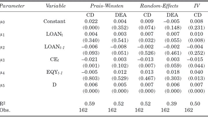
Estimation results are reported for the Cobb Douglas cost efficiency estimates and the DEA scores. The results are presented in columns 3 and 4 of Table 8. From the results, it would appear that the parametric approaches yield cost efficiency scores, which are compatible with the Berger and DeYoung (1997) ‘bad management’ hypothesis i.e. an increase in cost efficiency reduces the credit institution’s levels of loan loss reserves relative to its total assets. The Cobb Douglas set of cost efficiency score coefficients are significant at the 1 per cent level. With the DEA generated score, however, the level of cost efficiency appears to be positivelyrelated to the level of loan loss reserves. We also find, across both models, that the non-building society credit institutions amongst the sample have significantly higher loan loss reserves.
To check the robustness of our results, we also estimate (9) as a random effects model. These results are reported in Table 8 (columns 5 and 6). We find broadly similar results for both the CD and DEA cost efficiency scores. Namely, the coefficient on the CD CE variable is negatively signed and significant at the 1 per cent level, while the DEA CE variable’s coefficient is positively signed and insignificant at the 5 per cent level. Finally, as our CE variables are only estimatesof individual credit institution’s cost efficiency, we seek to control for the ensuing ‘errors in variables’ issue. Accordingly, we instrument for the CD CE variables. The instrumental variable model adopted is the error components two stage least squares (EC2SLS) model proposed by Baltagi (1981). As an instrument we choose the ratio of total employees to total assets on the basis that an increase in employee numbers, ceterus paribus, would lead to a reduction in cost efficiency. An examination of the cost scores achieved suggested a relatively strong correlation between the scores and the total employees ratio (of approximately 74 per cent).23We also explored the
use of both the ratio of financial and physical capital to total assets and lagged values of CE as alternative instruments, however, the initial first-stage regressions suggested that the ratio of total employees appeared to be a stronger instrument. The results of this estimation are reported in the final
22The estimation was carried out using Stata 8.0.
column of Table 8. It is evident that the IV results are quite similar to the random effects model estimated with the CD’s cost efficiency variable (column 5 of Table 8). The respective CE variables’ coefficients differ in magnitude only marginally and the cost efficiency variable is still significant (at the 5 per cent level) under the two-stage model. Overall, therefore, in the case of the parametric efficiency score, there would appear to be some evidence of a negative relationship between cost efficiency levels and the loan loss provision levels within the sample of institutions.
V CONCLUDING COMMENTS
[image:19.498.67.426.111.314.2]This paper generates a series of efficiency scores for a sample of Irish and British credit institutions over the 1996-2001 time period. Efficiency scores are estimated/calculated with parametric and non-parametric methods and the results are then compared with nonfrontier indicators of banking performance. Results suggest that the sample exhibit inefficiencies in production costs – although the degree of inefficiency is at the lower bound of international results reviewed by Berger and Humphrey (1997). Parametric Table 8: Second Stage Estimates of Non-Frontier Indicators and Efficiency
Scores
Parameter Variable Prais-Winsten Random-Effects IV
CD DEA CD DEA CD
µ0 Constant 0.022 0.004 0.009 –0.005 0.008
(0.000) (0.352) (0.074) (0.148) (0.231)
µ1 LOANt 0.004 0.003 0.007 0.007 0.010
(0.340) (0.541) (0.032) (0.055) (0.008)
µ2 LOANt-1 –0.006 –0.008 –0.002 –0.002 –0.004
(0.093) (0.051) (0.526) (0.461) (0.252)
µ3 CEt –0.021 0.003 –0.013 0.003 –0.015
(0.001) (0.102) (0.007) (0.059) (0.044)
µ4 EQYt-1 –0.005 0.012 0.013 0.018 0.040
(0.803) (0.529) (0.467) (0.303) (0.013)
µ5 D 0.006 0.005 0.007 0.006 0.007
(0.000) (0.000) (0.000) (0.000) (0.000)
R2 0.59 0.52 0.52 0.39 0.50
Obs. 162 162 162 162 162
scores give an indication of the ranking of credit institutions’ average efficiency over the period, as well as an indication of whether that average efficiency is improving, or disimproving over time. Our econometric results suggest that the degree of inefficiency has been falling over the period. As such, these results are somewhat in agreement with non-parametric results for UK credit institutions in studies by Drake (2001) and Drake and Simper (2003) for similar time periods. Unlike other studies, however, non-parametric inefficiency scores are closely aligned, in magnitude, to those of the econometric estimation. Both sets of scores suggest that large credit institutions are more efficient than smaller institutions in the sample. We also find evidence of increasing returns to scale within the sample. Irrespective of the method used, we find that average efficiency levels for UK credit institutions are at least 4 per cent greater than that of Irish institutions. This result is reinforced by additional cost function estimates, which reveal, on average, higher significant costs for Irish credit institutions vis-à-vistheir UK counterparts.
The second exercise of relating inefficiency scores to other indicators is an increasing feature of studies examining the efficiency of the credit institution sector. We find, that parametric estimates of cost efficiency are negatively related to the level of loan loss reserves. This result holds for different panel data estimators and as such, we believe, this link could be further explored in future research. DEA generated scores, on the other hand, under the same hypothesis, have a counter-intuitive effect. However, this result is tempered somewhat by the size of the sample used in the non-parametric approach.
Increasingly, in these second stage models, individual efficiency scores are not only used to characterise the performance of the credit institution itself, but are also used to reveal information pertaining to the overall structure of the market within which financial institutions operate. Vander-Vennet (2002) for instance, uses stochastically generated efficiency scores as a determining variable within the structure-conduct-performance (SCP) paradigm, in examining credit institution performance and market structure. Future work could explore this issue in greater detail.
REFERENCES
BALTAGI, B., 1981. “Simultaneous Equations with Error Components”, Journal of Econometrics, Vol. 17, pp. 189-200.
BARR, R., L. SEIFORD, and T. SIEMS, 1994. “Forecasting Bank Failures: A Non-Parametric Frontier Estimation Approach”, Recherchés Economiques de Louvain, Vol. 60, pp. 417-429.
Efficiency and Panel Data”, The Journal of Productivity Analysis, Vol. 3, pp. 153-169.
BATTESE, G. and T. COELLI, 1993. “A Stochastic Frontier Production Incorporating a Model for Technical Inefficiency Effects”, Working Paper 69, Department of Econometrics, University of New England.
BATTESE, G. and G. CORRA, 1977. “Estimation of a Production Frontier Model: With Application to the Pastoral Zone of Eastern Australia”, Australian Journal of Economics, Vol. 21, pp.169-179.
BAUER, P., A. BERGER and D. HUMPHREY, 1998. “Consistency Conditions for Regulatory Analysis of Financial Institutions: A Comparison of Frontier Efficiency Techniques”, Journal of Economics and Business, Vol. 50, pp. 85-114.
BERGER, A. and R. DEYOUNG, 1997. “Problem Loans and Cost Efficiencies in Commercial Banks”, Journal of Banking and Finance, Vol. 21, pp. 849-870. BERGER, A. and D. HUMPHREY, 1997. “Efficiency of Financial Institutions:
International Survey and Directions for Future Research”, European Journal of Operational Research, Vol. 98, pp. 175-212.
BERGER, A. and L. MESTER, 1997. “Inside the Black Box: What Explains Differences in the Efficiencies of Financial Institutions?”, Working Paper 97-1, Federal Reserve Bank of Philadelphia.
BIKKER, J., 2002. “Efficiency and Cost Differences Across Countries in a Unified European Banking Market”, Staff Report 87, De Nederlandsche Bank.
CARBO, S., E. GARDENER and J. WILLIAMS, 2003. “A Note on Technical Change in Banking: The Case of European Banks”, Applied Economics, Vol. 35, pp.705-719. CAZALS, C., J. FLORENS and L. SIMAR, 2002. “Nonparametric Frontier Estimation:
A Robust Approach”, Journal of Econometrics, Vol. 106, pp.1-25.
CHARNES, A., W. COOPER, A. LEVIN and L. SEIFORD, 1995. Data Envelopment Analysis: Theory, Methodology and Applications, Boston, USA: Kluwer Academic. CLARK, J. and T. SIEMS, 2002. “X-efficiency in Banking: Looking Beyond the Balance
Sheet”, Journal of Money Credit and Banking, Vol. 34, pp. 987-1013.
COELLI, T., D. PRASADA-RAO and G. BATTESE, 1998. An Introduction to Efficiency and Productivity Analysis, Boston, USA: Kluwer Academic.
CUMMINS, J. and M. WEISS, 1998. “Analyzing Firm Performance in the Insurance Industry using Frontier Efficiency Methods”, Technical Report, University of Pennsylvania, Philadelphia, PA: The Wharton School.
DRAKE, L., 2001. “Efficiency and Productivity Change in UK Banking”, Applied Financial Economics, Vol. 11, pp. 557-571.
DRAKE, L. and R. SIMPER, 2003. “Competition and Efficiency in UK Banking: The Impact of Corporate Ownership Structure”, Economic Paper ERP03-07, Loughborough University.
EISENBEIS, R., G. FERRITER and S. KWAN, 1999. “The Informativeness of Stochastic Frontier and Programming Frontier Efficiency Scores: Cost Efficiency and Other Measures of Bank Holding Company Performance”, Working Paper 99-23, Federal Reserve of Atlanta.
FARRELL, M., 1957. “The Measurement of Productive Efficiency”, Journal of the Royal Statistical Society, Vol. 120, pp. 253-281.
FRAIN, J., 1990. “Efficiency in Commercial Banking”, Research Technical Paper
GLASS, J. and D. MCKILLOP, 1992. “An Empirical Analysis of Scale and Scope Economics and Technological Change in an Irish Multiproduct Bank”, Journal of Banking and Finance, Vol 16, No. 2.
HASAN, I. and L. WALL, 2003. “Determinants of the Loan Loss Allowance: Some Cross-Country Comparisons”, Discussion Paper 33, Bank of Finland.
HUGHES, J., L. MESTER and C. MOON, 2000. “Are all Scale Economies in Banking Elusive or Illusive: Evidence Obtained by Incorporating Capital Structure and Risk Taking into Models of Bank Production”, Working Paper 00-33, University of Pennsylvania, Philadelphia, PA: The Wharton School.
KWAN, K. and R. EISENBEIS, 1996. “Bank Risk, Capitalization and Efficiency” Working Paper 96-35, University of Pennsylvania, Philadelphia, PA: The Wharton School.
LAVEN, L. and G. MAJNONI, 2002. “Loan Loss Provisioning and Economic Slowdowns: Too Much Too Late?” Mimeo, The World Bank.
LOVELL, C., 1993. “Linear Programming Approaches to the Measurement and Analysis of Productive Efficiency” Working Paper, Department of Economics, Georgia College of Business Administration, Georgia, USA.
LUCEY, B., 1993. “Profits, Efficiency and Irish Banks”, Journal of the Statistical and Social Inquiry of Ireland, Vol. 27, pp. 31-83.
MCKILLOP, D. and J. GLASS, 1991. “Multi-product Cost Attributes – A Study of the Irish Banking Industry 1972-1988”, Working Paper AF/91-1. Belfast. The Queens University.
PAIN, D., 2003. “The Provisioning Experience of the Major UK Banks: A Small Panel Investigation”, Working Paper 177, Bank of England.
PASTOR, J., 2002. “Credit Risk and Efficiency in the European Banking System: A Three-Stage Analysis”, Applied Financial Economics, Vol. 12, pp. 895-911. PRAIS, S. and C. WINSTEN, 1954. “Trend Estimators and Serial Correlation”,
Discussion Paper 383, Cowles Foundation.
RESTI, A., 1997. “Evaluating the Cost-Efficiency of the Italian Banking System: What Can be Learned from the Joint Application of Parametric and Non-Parametric Techniques”, Journal of Banking and Finance, Vol. 21, pp. 221-250.
ROGERS, K., 1998. “Nontraditional Activities and the Efficiency of US Commercial Banks”, Journal of Banking and Finance, Vol. 22, pp. 167-182.
SEIFORD, L., 1996. “Data Envelopment Analysis: The Evolution of the State of the Art (1978-1995)”, Journal of Productivity Analysis, Vol. 7, pp. 99-138.
VANDER-VENNET, R., 2002. “Cost and Profit Efficiency of Financial Conglomerates and Universal Banks in Europe”, Journal of Money, Credit and Banking, Vol. 34, pp. 254-282.
WHEELOCK, D. and P. WILSON, 1995. “Explaining Bank Failures: Deposit Insurance, Regulation and Efficiency”, Review of Economics and Statistics, Vol. 77, pp. 689-700.
WHEELOCK, D. and P. WILSON, 1999. “Technical Progress, Inefficiency and Productivity Change in US Banking, 1984-1993”, Journal of Money, Credit and Banking, Vol. 31, pp. 212-234.