Attractive energy and entropy or particle size: the yin and yang of physical and biological science 1

Attractive energy and entropy or particle size: the yin and

yang of physical and biological science

Douglas Henderson

Department of Chemistry and Biochemistry, Brigham Young University, Provo UT 84602, USA

1

Abstract

1 Introduction

In a mechanical system, the equilibrium state is the state of lowest energy, E. For example, a ball will sit at the bottom of an energy well or bowl. However, what happens if the table on which the bowl is placed shakes, perhaps due to an earthquake (a common occurrence in the western US)? The ball will, on average, be in a higher energy state and no longer always be at the bottom of the bowl. The counterpart of the earthquake in a thermodynamic system is the temperature, T. Equilibrium in a thermodynamic system is the state of lowest free energy, which in a TVN system (V is the volume, and N is the number of particles) is =A E TS , where A

and S are the Helmholtz free energy and entropy. The Helmholtz function and the entropy are related by

= A.

S

T  

 (1)

Thus, thermodynamic equilibrium is established by a competition or balance between decreasing E and increasing S (or at least TS). This balance is remarkably similar to the Toaist concept of yin and yang, yin being a downward influence and yang being an upward influence, where harmony, or balance, in life is achieved through balancing yin and yang.

The concept of entropy was established by Clausius and others in the mid nineteenth century and its tendency to increase was understood by them. However, our modern understanding of the relation of entropy to the disorder of a system was established by Boltzmann towards the end of the nineteenth century. The genius of Boltzmann was not realized at that time and perhaps is not fully realized today. Boltzmann was criticized because his ideas contradicted deterministic Newtonian mechanics. His work anticipated non-deterministic mechanics, which is only now being broadly developed. Because of the revolutionary and far reaching character of Boltzmann's work, he is a first tier scientist, similar to Newton, Maxwell, and Einstein. It is sad that Boltzmann became depressed because of the criticism of lesser, but politically more powerful, scientists and ended his life.

2 van der Waals

This article will focus on liquids. Firstly, this is because I was attracted to the study of liquids because, when I was young, it was believed that, in contrast to gases and solids, there was no useful theory of liquids. Indeed, as a graduate student I recall reading an essay by Joe Hirschfelder in which the lack of a theory of liquids was stated to be a major bottleneck in physical science. Secondly, biophysics has emerged as an exciting field for physical scientists. There may be exceptions, but most biology occurs in liquids (water or an aqueous solution) or at the interface of a liquid and a solid.

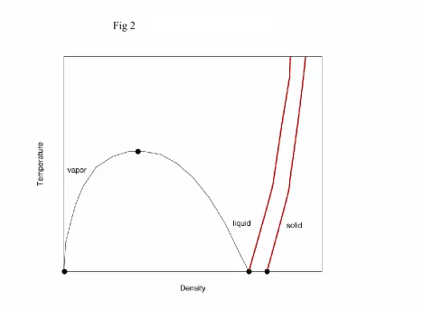
second order. The region in Figs. 1 and 2 with T below Tc (but above the triple point

temperature, Tt) and above the critical density, c, (but below the densities of the solid-fluid

transition) is generally called the liquid state and the remaining region (again below the densities for solid-fluid coexistence) is generally called the gaseous state. This is a poor terminology. A gas will occupy all the available volume whereas a liquid will not. A liquid is characterized by a free surface. Thus, only the high density fluid along the liquid-vapor equilibrium curve is clearly a liquid. It would be best to reserve the terms liquid and vapor for the high and low density fluids that are in liquid-vapor equilibrium, respectively, and regard the fluid in the remaining region, outside the solid state, as a fluid or gas. However, this careless terminology is so ingrained that it is likely fruitless, perhaps even pedantic, to attempt a reformation. In any case, there is a continuity of states. By increasing T then a compression followed by a lowering of the temperature, a vapor can pass continuously to a liquid and vice versa. Of course, we are all aware that the phase diagram in Figs. 1 and 2 are for a simple fluid. Water is more complex. At low temperatures, liquid water is more dense than ice. Indeed, although this is annoying if an automobile radiator freezes, aquatic life would not be possible in colder climates if this were not true. Still, for our discussion this is a detail. The above discussion is applicable to water/water vapor equilibrium.

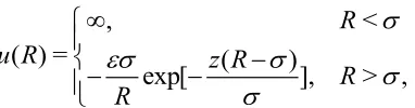
Presumably, van der Waals (vdW) was aware of Andrews work. In any case, vdW thought of the intermolecular interactions between fluid molecules as being attractive at long range and repulsive at short range. This is illustrated, for spherically symmetric molecules, in Fig. 3 with the Yukawa intermolecular pair interaction,

, <

( ) = _{( )}

exp[ ], > ,

R

u R _{z R}

R R    _      _{ }  (2)

where R is the separation of the centers of a pair of molecules,  is the molecular diameter, and  is the strength of the energetic interaction at contact. In the case of the Yukawa potential, this is also the minimum of the pair potential. The parameter z determines the range of the potential. The Yukawa potential is only qualitatively reasonable as a representation of the interparticle potential. However, the thermodynamic properties of a simple fluid are determined largely by the area of the potential curve that can be given accurately by adjusting z. The value

z=1.8 is appropriate for most liquids (Henderson et al, 1978) Starting with the ideal gas equation,

= ,

pV NkT (3)

or equivalently,

0 _{= 3ln 1 ln ln ,}

A

N V

NkT    (4)

where k is the Boltzmann constant (the gas constant per molecule) and 1/2 = / (2h mkT)

  with

h and m being Planck's constant and the molecular mass, vdW approximated the contribution of the repulsive term, due to  , as resulting in a reduced available volume (or free volume),

0 =

NkT p

V Nb (5)

and

0 _{= 3ln 1 ln ln( ).}

A

N V Nb

NkT     (6)

The subscript 0 is used to emphasize that p0 and A0 are the hard sphere contributions to p and

A. Van de Waals regarded the contribution of the attractive forces as an internal pressure that held the fluid together (after all, liquids can exist at atmospheric pressures that are quite small). Since the internal pressure would surely vanish at low density, there is every reason to expect that a reasonable approximation would be

= Aid ln(1 ) ,

A a

b

NkT NkT kT

 

   (7)

where the subscript id indicates that the quantity is the ideal gas term. Since

= A,

p

V  

 (8)

the famous van der Waals equation,

2 2

= NkT N a,

p

V Nb  V (9)

results. It will be helpful to write this as

2

0 2

= N a.

p p V

 (10)

The entropy is given by Eq. (1). Differentiation with respect to T yields

= Sid ln(1 )

S

b

Nk Nk   (11)

and

= Eid .

E Na

NkT NkT VkT (12)

liquid at high densities. The vdW pressures are too large, often by an order of magnitude compared to the experimental results (Hsu and McKetta, 1964).

One notable feature of the vdW equation is that it predicts a law of corresponding states. That is,

/ c = ( / , / ),c c

p p f V V T T (13)

where f is some function. Thus, the equations of state of various similar fluids can be scaled so that they become one equation. This is a good approximation for many liquids although such effects as molecular shape prevent such a simple relation from being exact. The vdW expression for f is in error but the concept of corresponding states is not.

Improvements were attempted. For example, Berthelot suggested

2 2

= NkT N a

p

V Nb V T  (14)

and Dieterici suggested

= NkT exp Na .

p

V Nb VkT

_ 

 

   (15)

The Dietericic equation yields a better value for pV NkT/ at the critical point. However, both the Berthelot and Dieterici equations fail at high densities. Because of this, for a century the vdW theory was regarded, incorrectly, as having only pedagogical interest.

Table 1 Equation of state of methyl chloride (Tc= 143.1



C, pc = 65.919 atm, = 2.755

c

V cm3_/gm)

T V p(expt1) p(vdW)

(

C) (cm3_{/gm) (atm) (atm)}

125 88.266 6.975 7.063

27.774 20.049 20.629

16.333 30.664 32.017

11.070 39.817 42.215

7.204 50.015 52.848

143.7 67.069 9.567 9.632

18.099 30.398 31.288

8.321 51.077 53.818

1.939 69.954 251.92

1.610 101.510 936.55

Even as late as the middle of the twentieth century, equations similar in form to that of vdW were suggested. For example, in the mid twentieth century Redlich and Kwong proposed the equation of state

2 1/2

= .

( )

NkT N a

p

V Nb T V V Nb   (16)

All of these attempted improvements retain the vdW free volume approximation, V Nb . Investigators were directing their attention to the wrong term. The problem with the vdW equation and its decendents was not the energy term involving a, but with the overly simplified free volume. The hard core term is treated crudely. This can be seen by returning to the hard sphere fluid, which would be described by Eq. (5) if the vdW equation were valid. Expanding Eq. (5) in powers of the density, = N V/ yields

2 3

0 _{= 1 ( ) ( ) .}

p V

b b b

NkT        (17)

This is a one dimensional approximation that neglects the fact that in higher dimensions, molecules can go around each other. The pressure can be expanded in a series in . In three dimensions,

2 3

0 _{= 1} 5_{( ) 0.2869( ) ,}

8

p V

b b b

NkT        (18)

with _{b= 2}3_{/ 3, where  is the hard sphere diameter.}

The vdW free volume grossly overestimates the hard sphere contribution to the pressure. This can be seen in Fig. 4. Since Eq. (18) was known in the nineteenth century, it seems quite amazing that the vdW free volume was retained for so long. A simple alternative,

0 4 1 = , (1 ) p V

NkT  (19)

3

= / 6

  can be constructed easily (Guggenheim, 1969). Equation (19) was known in the nineteenth century and was rediscovered about forty years ago. The vdW expression correctly reproduces only the first correction, called the second virial coefficient, to the ideal gas expression for pV NkT/ , whereas Eq. (19) reproduces the second and third virial coefficients correctly and gives a reasonable estimate of the higher virial coefficients. An even better approximation is the CS equation (Carnahan and Starling, 1965),

2 3 0 3 1 = . (1 ) p V NkT         (20)

hard sphere equation of state gives values for the pressure that are much too large. In contrast, the results of Eqs. (19) and (20) are much better. The CS result is very accurate. Much better results can be obtained using Eq. (10) but with some better expression for p₀, say the CS expression (Longuet-Higgins and Widom, 1965). Thus, we could regard

2 3 2 3 1 = (1 )

p kT     a 

   _

 (21)

as an improved or modified vdW equation.

The reason the vdW expression for p0 was retained so long was the fact that, with the

vdW free volume approximation, the vdW equation of state is a cubic equation that can be solved analytically. Before the advent of digital computers and, more especially, inexpensive personal computers, computations based upon the more accurate formulae were very time consuming. Perhaps the use of the vdW free volume is understandable for practical computations. However, it is very surprising that research scientists did not realize the the vdW theory was the basis of the desired theory of liquids and not just something for professors to mention in their lectures.

To cast this in terms of the aforementioned balance or competition between energy and entropy, note that in the vdW equation of state and in many of its extensions, the attractive forces, through the parameter, a, contribute exclusively to E and the repulsive forces (or particle size), through the parameter b, contribute exclusively to the entropy. This separation of energetic and entropic terms is absolute in the vdW theory. It is not absolute in more accurate theories that will now be considered but is still a good approximation.

3 Perturbation theory

Perturbation theory provides the formalism whereby the vdW can be made systematic and extensions developed. Perturbation theory (at least to first order) was developed by Zwanzig and Longuet-Higgins but was regarded as a high temperature theory that was useful only for gases. It was BH (Barker and Henderson, 1967a) who first realized that perturbation theory was useful for liquids and then estimated and calculated the second order term.

Considering first a pair potential with a hard core such as, for example. the Yukawa potential, the Helmholtz function can be expanded in powers of  , where  =1/kT . The result is

0 =1

= ( )n ,

n n

A A 



where A0 is, as before, the Helmholtz function of the unperturbed hard sphere system and the

n

A , for > 0n , give the effect of the perturbing attractive potential. The CS expression for A0 is

0 2 4 3 = . (1 ) id A A NkT NkT       (23)

However, all evidence indicates that this expansion is convergent for liquid temperatures between the critical and triple point temperatures. The first order term is easily obtained [7] and is given by

2 1

0 ( )

= 2 ( ) ,

A u R

g R R dR NkT   

 

 

 



where  is the depth of the pair potential, u R( ). The function g R( ) is the pair correlation function, a radial distribution function (RDF) in the case of spherical particles, that gives the probability of finding a particle a distance R from a central particle, normalized to unity at large

R. The subscript 0 indicates that g R0( ) is the RDF for the unperturbed hard sphere fluid. A

typical hard sphere RDF is shown in Fig. 5. The central molecule is surrounded by about 12 nearest `neighbors' (nn) at a distance of about  . In a solid the nearest neighbor distance (nnd) would be almost exactly  and the nn peak would be nearly a delta function. However, in a fluid, the nnd is diffuse. The nn's tend to exclude molecules further out and produce a minumum. The neighbors of neighbors produce further maxima and minima of diminishing strength. The asymptotic value, as R becomes large, of a RDF is 1 because the particles are uncorrelated at large R.

The term A1 is plotted in Fig. 6 for the Yukawa potential. This curve is typical of the A1

that is obtained using other ( )u R . At low densities, the higher order An have the form (Barker

and Henderson, 1967a),

1

2 0

( 1) ( )

= 2 ( ) .

n n

n

A u R

g R R dR

NkT n   

 _

   _

 

 



The remaining terms are higher order in  and involve higher order correlation functions. Barker and Henderson argued that these higher order terms are small, especially at high densities and that the second order term, A NkT2/ is, to a good approximation, proportional to the

compressiblity of the unperturbed hard sphere fluid. They called this a compressiblity approximation. A simple version of a compressiblity approximation for A2 is

2 2 2 0 0 ( ) = ( ) .

A u R

kT g R R dR

NkT p 

          _{   }   

 



The subscript 0 in the compressiblity indicates that the unperturbed hard sphere compressiblity is used. Using the CS equation of state,

4

2 3 4

0

(1 )

= .

1 2 2 10

kT p           _  _{   }

  (27)

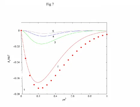
The results obtained from Eqs. (26) and (27) using the Yukawa potential are very similar to the results shown in Fig. 7 for A2 that were obtained using more refined methods. Although the

compressiblity approximation is simple, it is quite accurate and subsequent approximations for

2

Again, A1 contributes to the energy but not the entropy. In first order, the entropy of the

fluid (or liquid) is that of a hard sphere fluid. The first order term is a background energy, determined from the structure of a hard sphere fluid that produces the internal pressure and provides a well in which the molecules move as if they were hard spheres. That is, to first order in A, the particles are distributed as if they were hard spheres. The task is to determine g R0( ).

This can be done by computer simulation or by means of some theory. The higher order An

contribute to both the entropy and energy. The division into terms that contribute only to the entropy or only to the energy is no longer true if higher order terms are included.

One simple approximation is g R₀( ) = 1 for >R . This yields

1 _{= ,}

A

a

NkT  (28)

with

2

= 2 ( ) .

a u R R dR



 





In the case of the Yukawa potential this gives

3 2

1

= 2 z .

a

z

  (30)

Since Eq. (28) is just the last term in the vdW result, Eq. (7), we can refer to g R0( ) = 1 as the

vdW approximation for A1.

The higher order An are increasingly difficult to compute. For example, the expression

for A2 involves two, three, and four particle correlation functions. Barker and Henderson

determined A2 by MC simulation as well as by a compressiblity approximation. An approximate

integral equation that permits the calculation of the An will be discussed in the next section. For

the moment, the point to be made is that for a hard core potential, such as the Yukawa potential, first order perturbation theory predicts that the entropy is determined by the hard core repulsive potential and the energy change is due to the attractive part of the pair potential. Equilibrium is established by a balance or competition between excluded volume or space and attractive energy.

4 Theories based on the Ornstein-Zernike relation

Integral equations provide an approximate method of calculating g R( ) and thermodynamics but also the higher order An. Most modern integral equation theories are based

on the Ornstein-Zernike (OZ) relation. To obtain this relation we observe first that subtracting its asymptotic value from ( )g R yields a correlation function, called the total correlation function, ( )h R = ( )g R -1. This function is not long ranged in the sense of the Coulomb potential but its range can extend over several molecular diameters.

12 12 13 23 3

( ) = ( ) ( ) ( ) ,

h R c R 



where ri is the position of the center of molecule i and Rij =|r ri j|. To keep things simple,

only spherically symmetric molecules have been considered. In the case of nonspherical molecules, an integration over angular variables is required. The integral in Eq. (31) is a convolution integral. If the Fourier transform is taken, such a convolution integral becomes the product of the Fourier transforms of the two terms in the integral. Thus, in Fourier space

2

( ) = ( ) ( ),

h k c k_ c k_{ (32)}

where k is the Fourier transform variable and not the Boltzmann constant. As soon as this discussion is completed, k will revert to representing the Boltzmann constant.

As the density is increased, the indirect function will involve chains of several molecules. This series is called a chain sum. Thus, in Fourier space,

2 2 3

( ) = ( ) ( ) ( )

h k c k c k  c k   (33)

or





( ) = ( ) 1 ( ) ( ) ... ,

h k c k_ c k_  c k_  ₍₃₄₎

which can be summed to yield

( ) ( ) =

1 ( )

c k h k c k      (35) or, equivalently, ( ) = ( ) ( ) ( ).

h k c k_ h k c k _{ (36)}

Converting back to coordinate space, we have the OZ relation

12 12 13 23 3

( ) = ( ) ( ) ( ) .

h R c R 

_

Originally, this relation was obtained to describe light scattering, especially near the critical point. However, during the past half century it has been realized that the OZ relation can be used to develop theories of fluids. By itself, the OZ relation is merely a definition of the DCF and does not give a method of determing ( )c R unless h r( ) is already known. To yield an approximation, the OZ relation must be coupled with some approximate relation, called a

closure because the closure yields a closed equation. If the molecules have a hard core, ie,

( ) =

u R  for <R . Therefore, we have the exact result,

( ) = 1

h R  (38)

( ) = ( ),

c R u R (39)

for R>. Equations (38) and (39), together with the OZ relation, permit the determination of ( )

c R and g R( ) = ( ) 1h R  . There is no reason to suppose, a priori, that the MSA is particularily accurate. However, a posteriori, it turns out to be quite accurate for many applications. Not only that, the MSA has an analytic solution for many systems. The accuracy of a closure is determined by comparison with simulations and experiment. Other criteria, such as the completeness of the set of terms in c R( ), have not proven to be very useful in assessing the accuracy of a closure.

The name mean spherical approximation conveys little. The origin of this name comes from the theory of lattice gases and, no doubt, once meant something. In any case, Eq. (39) is exact at large R and Eq. (38) is the exact hard core condition. The MSA can be considered to be a hard core approximation that is correct at large R.

It is worth mentioning that for the hard sphere fluid, the MSA consists of Eq. (38) together with

( ) = 0

c R (40)

for > 0R . It is interesting to note that this is exactly the Percus-Yevick (PY) approximation for a hard sphere fluid. The PY approximation and the MSA are identical for hard spheres. However, they are different approximations for other fluids. Generally speaking, the PY approximation has been found to be less useful than the MSA and will not be considered further.

One such system, for which the MSA has an analytic solution, is the Yukawa fluid. The MSA has been solved for the Yukawa fluid (Waisman, 1973). However, his result is implicit, involving the numerical solution of six simultaneous nonlinear algebraic equations in six unknown variables. Subsequently, (Henderson et al, 1995) obtained explicit results for the thermodynamics by expanding the solution in a perturbation expansion. They obtained Eq. (23) for A0 and

1 ₌ ( ) _,

12 [ ( ) exp( ) ( )]

A zL z

NkT  L z  z S z (41)

where L z( ) and S z( ) are polynomials that are given by

( ) = 12 [1 2 (1 ) ]

2

L z     z (42)

and

2 2 2 3

( ) = 12 (1 2 ) 18 6 (1 ) (1 ) .

S z       z   z   z (43)

Equation (41) can be obtained by the method of Henderson et al but can also be obtained from the PY result for g R₀( ) that was derived earlier (Wertheim, 1964).

The expressions for the higher order A_n are complex but are easily calculated. Also it is easy to differentiate the A_n analytically to obtain corresponding expressions for the pressure. Results obtained from the MSA and MC simulation (using =1.8z , which is appropriate for many fluids) are given for A1 through A5 in Figs. 6 and 7. It is virtually impossible to obtain

vdW theory, Eq. (21) or (28), A1 should be the dominant term. This, certainly, is seen to be the

case in Figs. 6 and 7. Also in a vdW theory, A1 should be a linear function of . This is not the

case but the departure from linearity is not so great. The extended vdW theory is a very reasonable starting point. The simple compressiblity approximation gives similar results for A2.

The terms A3 through A5 are always negative (in the MSA, at least) even though it might seem

in Fig. 7 that there is a change of sign. In the MSA, the An for n>2 lack a term that is linear in

. This is not correct. It is an error in the MSA but is not a serious problem since these higher order terms are small. Additionally, most interest is for dense fluids.

Again it is to be emphasized that if the perturbation series is terminated at A1, then A0,

which results from the hard core repulsion, determines the entropy and the contribution of the attractive forces is given by A₁. While energy and entropy are mixed through the higher order

n

A , these higher order terms are small, especially at high densities. The competition between space and attractive forces produces the balance between energy and entropy and minimizes the free energy.

5 Real molecules are not hard

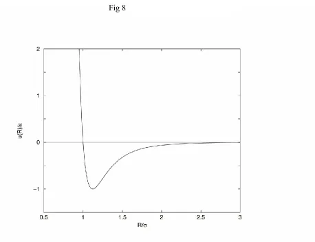
In the vdW theory, the modified vdW theory, the MSA, and the perturbation theory discussed so far, the molecules are considered to have hard cores. Real molecules have soft cores. For example, a popular model for a fluid is the Lennard-Jones (LJ) fluid, where the intermolecular potential is given by the LJ 12-6 potential,

12 6

( ) = 4 .

u R R R   _ _{ }  _{ } _      

  (44)

The parameter  is now the depth of the potential and  is the value of R for which the potential changes sign. The LJ 12-6 potential is plotted in Fig. 8. The LJ 12-6 potential is more reasonable than the Yukawa potential because its repulsive region is not infinitely hard and its long range attraction decays correctly as _R6_{, as is predicted by quantum theory, rather than}

exponentially. Although an improvement, the LJ 12-6 potential is not a complete representation of the interaction between real molecules. In the case of argon, the depth of the actual interaction is somewhat larger and the the coefficient of the _R6 _{is somewhat smaller than the LJ 12-6}

potential suggests. Even so, the Yukawa potential (z=1.8), the LJ 12-6 potential, and more realistic potentials yield similar thermodynamic properties.

Thus, real molecules are not hard. However, the repulsive region is very steep and a hard core representation is very reasonable. In fact, it has been shown (Barker and Henderson, 1967b) that such steep repulsions are accurately represented by a hard sphere potential whose diameter is given by





0

( ) = 1 exp[ ( )] .

d T



through first order in the perturbation series is no longer exact. However, this is a small effect. The RDF of a LJ 12-6 fluid is plotted in Fig. 9 and compared with the hard sphere RDF. It is seen that the hard sphere and LJ RDF's are quite similar. In Fig. 10, the pressure of a LJ 12-6 fluid, calculated from second-order perturbation theory is compared with computer simulations. The agreement is very good.

Subsequently, a useful alternative method for dealing with molecules with a soft core has been developed (Weeks et al, 1971a,b)

6 Electrolytes

A simple model for electrolytes is the primitive model in which the ions are modeled as charged hard spheres and the solvent is modeled as a dielectric continuum, whose dielectric constant is given by  (not to be confused with the energy parameter in the intermolecular potentials discussed above). The idea behind the representation of the solvent by a continuum is that the electrolyte is dilute and the ions are far apart and do not sense the molecular nature of the solvent. Thus, the primitive model is useful for low concentrations. The formalism developed so far is applicable to electrolytes except that we should substitute ion for molecule. The ion-ion potential in the primitive model is

2

, <

( ) =

, > ,

ij

i j

ij R u R _{z z e}

R R         (46)

where zi and i are the valence and diameter of an ion of species i and ij = i j. The

parameter e is the magnitude of the electronic charge.

The standard theory for an electrolyte is the DH theory (Debye and Hückel, 1923). Conventionally, this theory is obtained by solving a differential equation, usually linearized, yielding the linearized DH or LDH theory. However, the LDH theory can also be obtained from the MSA or even a chain sum, assuming that the ions are point ions, i.e., i = 0 (Henderson,

1983). The resulting LDH mean activity coefficient is

2

ln =| | ,

2

z z e kT

 



   (47)

where

2

2 ₌ 4 2 _.

i i e z   





Note that the properties of the electrolyte are typically functions of _1/ 2

and/or _T1/2_{; this is in}

contrast to the fluids considered so far, where  and T appear with integral powers.

are seen in both theory and experiment as the concentration is increased. However, for variety, the rate constant for an electrochemical reaction can be examined. Reaction rate constants have been calculated using the MSA (Fawcett et al, 1997). A typical result is shown in Fig. 11. At low concentrations the rate constant is a linear function , or _I1/2_{, where I is the ionic strength,}

but deviations are seen as the concentration or ionic strength is increased. The MSA result is in good agreement with experiment. The main point is that good results are obtained only when the ion cores are taken into account. In contrast to simple fluids, the ion cores in an electrolyte contribute to both the energy and entropy. The competition is between charge and size but the principle remains.

7 Channel selectivity

Ion channels are essential for the proper functions of cells. An ion channel is a protein with a hole through which ions pass selectively. We will consider sodium and calcium channels. Calcium channels play an important role in such physiological functions as muscle contraction. A calcium channel will conduct Ca2 _{ions when these ions are present in micromolar or larger}

concentrations even if other ions, say Na_{, are present in much larger concentrations whereas the}

sodium channel does not exhibt such a preference.

A simple intuitive model (Nonner et al, 2000), based on the MSA for a bulk electrolyte, in which the selectivity of a calcium channel is produced by the competition between the attractive Coulombic forces between the cations and the negatively charged structural elements, glutamates in what is called a EEEE locus, and the size of the ions and glutamates. A model representation of a calcium channel is shown in Fig. 12, where p and w are the delectric

coefficients of the protein and the solvent, respectively. The large red spheres in Fig. 12 are the oxygens of the glutamates, each with a single negative charge (-e). Since the glutamates are flexible, but attached to the channel protein, the oxygens are confined to the channel but are free to move within the channel. In the EEEE locus there are four glutamates with a negative charge of 4 e.

In this competition, the ions are attracted into the channel but because of the restricted geometry of the channel filter and the excluded volume of the ions and glutamates, the Ca2 _ions

are more effective at balancing the -4e charge of the four glutamates than are the Na _{ions since}

they deliver twice the charge while occupying almost the same volume.

As is seen in Fig. 13, this charge/size competition (CSC) model accounts (Boda, et al, (2007) very well for the selectivity of a DEEA calcium channel, whose structural elements are (A) aspartate (-e), (E) glutamate (-e), (A) alanine (neutral), with a net charge of -3e and for the DEKA sodium channel, whose structural elements are aspartate, glutamate, (K) lysine (+e), and alanine (called a DEKA locus) with a net charge of -e. Because there is little negative charge to balance, the Na ions are quite effective at balancing the DEKA charge and the sodium channel is not Ca selective. A simple mutation of K into E changes the net charge from -e to -3e and turns the sodium channel into a calcium channel. Results have been obtained for the EEEE calcium channel (Boda et al, 2009).

8 Summary

It is now well understood that both the molecular size and attractive energy must be taken into account accurately to describe the properties of materials. Examples illustrating this are given from the theory of simple liquids, electrolytes and the selectivity of ion channels. Although this is understood in physical science, it seems less well understood in biological science. For example, the transport of ions is often described by the Nernst-Poisson approach which, like the Debye-Hückel theory, neglects the ion cores. Just as there must be a balance of yin and yang for harmony in life, there must be a balance of size or space or entropy and attractive energy in physical or biological science. It will be interesting to determine by simulation studies the extent to which these concepts are useful in understanding complex systems, such as protein molecules in aqueous solution.

Acknowledgments

The author is grateful for the support and assistance of his colleagues over the years. Indeed, in many cases the author was the assistant. It is difficult to name all these collaborators. However, Henry Eyring, John Barker, Farid Abraham, Lesser Blum, Ron Fawcett, Andrij Trokhymchuk, Dezsö Boda, Dirk Gillespie, Wolfgang Nonner, and Bob Eisenberg deserve particular mention. The work of the author reviewed here was performed at the CSIRO Chemical Research Laboratories in Melbourne, Australia, the University of Waterloo, Canada, the IBM Research Laboratory in San Jose, California, USA, the University of Utah in Salt Lake City Utah, USA, and Brigham Young University in Provo Utah, USA. The ion channel work was performed using the facilities of the Ira and Marylou Fulton Supercomputing Center at Brigham Young University. The author's trip to Linz was made possible by the support of the Austrian Academy of Science and the University of Linz. Alexis Hales assisted in the preparation of some of the figures. Bob Eisenberg read this manuscript and made useful suggestions.

References

[1] Barker, J.A., Henderson, D. 1967a. Pertubation theory and equation of state for fluids: the square-well fluid. J. Chem. Phys. 47, 2856-2861.

[2] Barker, J.A., Henderson, D. 1967b. Perturbation theory and equation of state for fluids. II. A successful theory of liquids. J. Chem. Phys. 47, 4714-4721.

[3] Barker, J.A., Henderson, D. 1971. Monte Carlo values for the radial distribution function of a system of hard spheres. Mol. Phys. 21, 187-191.

[4] Blum, L. 1980. Primitive electrolytes in the mean spherical approximation. Theor. Chem. 5, 1-66.

Steric Selectivity in Na channels arising from protein polarization and mobile side chains. Biophys. J. 93, 1960-1980.

[6] Boda, D., Nonner, W., Henderson, D., Eisenberg, B., Gillespie, D. 2009. In preparation.

[7] Carnahan, N.F., Starling, K.E. 1969. Equation of state for nonattracting hard spheres. J. Chem. Phys. 51, 635-636.

[8] Debye, P., Hückel, E. 1923. Zur theorie der electrolyte I. Gefrierpunktserniedrigung und verwandte erscheinungen. Physikalische Zeit. 24, 185-206.

[9] Fawcett, W.R., Tikanen, A.C., Henderson, D. 1997. The mean spherical

approximation and medium effects in the kinetics of solution reactions involving ions. Canadian J. Chem. 75, 1649-1655.

[10] Guggenheim, E.A. 1965. The new equation of state of Longuet-Higgins and Widom. Mol. Phys. 9, 43-47.

[11] Henderson, D. 1983. Perturbation theory, ionic fluids, and the electric double layer. In: Haile, J.M., Mansoori, G.A. (eds) Molecular-based study of fluids, ACS Adv. in Chemistry, vol. 204, ACS, Washington, pp. 48-71, see Eqs. 41-46.

[12] Henderson, D., Blum, L., Noworyta, J.P. 1995. Inverse temperature expansion from the solution of the mean spheical approximation integral equation for a Yukawa fluid. J. Chem Phys. 102, 4973-4975.

[13] Henderson, D., Waisman, E., Lebowitz, J.L., Blum, L. 1978. Equation of state of a hard core fluid with a Yukawa tail. Mol. Phys. 35, 241-255.

[14] Hsu, C.C., McKetta, J.J. 1964. Pressure-volume-temperature properties of methyl chloride. J. Chem. Eng. Data 9, 45-51.

[15] Longuet-Higgins, H.C., Widom, B. 1965. A rigid sphere model for the melting of argon. Mol. Phys. 8, 549-556.

[16] Nonner, W., Catacuzzeno, L., Eisenberg, B. 2000. Binding and selectivity in L-type Ca channels: a mean spherical approximation. Biophys. J. 79, 1976-1992.

[17] Waisman, E. 1973. The radial distribution function of a fluid of hard spheres at high densities. Mean spherical integral equation approach. Mol. Phys. 25, 45-48.

[18] Waisman, E., Lebowitz, J.L. 1970. Exact solution of an integral equation for the structure of a primitive model of electrolytes. J. Chem. Phys. 52, 4307-4309.

charged hard spheres. I. Method of solution. J. Chem. Phys. 56, 3086-3093.

[20] Waisman, E., Lebowitz, J.L. 1972b. Mean spherical model integral equation for charged hard spheres. II. Results. J. Chem. Phys. 56, 3093-3099.

[21] Weeks, J.D., Chandler, D., Andersen, H.C. 1971a. Role of repulsive forces in determining the equilibrium structure of simple liquids. J. Chem. Phys. 54, 5237-5247.

[22] Weeks, J.D., Chandler, D., Andersen, H.C. 1971b. Perturbation theory and the thermodynamic properties of simple liquids. J. Chem. Phys. 55, 5422-5423.

Figure 1: Pressure-temperature cut of the phase diagram of a typical simple fluid. The solid, liquid, and vapor phases are separated by three coexistence curves that meet at the triple

point. The liquid-vapor curve ends with the critical point.

Figure 2: Temperature-density cut of the phase diagram of a typical simple fluid. The lowest temperature is the triple point temperature and the three coexisting phases are marked by circles. The (black) parabolic-like curve gives the liquid-vapor coexistence curve with the critical

point, marked by a circle, at the maximum. The region below this curve is a metastable/unstable region. The rapidly rising (red) curves are the solid-fluid coexistence curves. The region between

these curves is a metastable/unstable region.

Figure 3: Yukawa intermolecular potential with z=1.8. The distance of closest approach of a pair of particles is =R  at which point the attractive interaction has its greatest magnitude,

( ) =

u  .

Figure 4: Equation of state of a hard sphere fluid. There is a branch for the hard sphere solid at higher densities. The dashed (blue), dot-dashed (red), and solid (black) curves give the

results of Eqs. 4, 17, and 18, respectively.

Figure 5: Typical radial distribution function of a dense hard sphere fluid. TheRDF of a Yukawa fluid is similar.

Figure 6: First order perturbation term for a Yukawa fluid with =1.8z . The points give the simulation values of Barker and Henderson while the curve gives the MSA result.

Figure 7: Higher-order perturbation terms for a Yukawa fluid with =1.8z . The curves are labeled with the appropriate value of =b n. The points are the simulation values of Barker

and Henderson while the curves give the MSA results.

Figure 8: The LJ 12-6 potential. Here =R  is the value for which u(R) changes sign. Since there is no hard core, there is no well defined distance of closest approach. However, a value of R that is somewhat smaller than  , determined from Eq. (42), is a reasonable measure

of the distance of closest approach.

Figure 9: Typical radial distribution function of a dense LJ 12-6 fluid. The rdf of the unperturbed reference hard sphere fluid, whose diameter is given by Eq. (42), is given by the

broken curve.

Figure 10: Equation of state of the LJ 12-6 fluid. The curves are isotherms whose corresponding values of kT/ are shown and the points are computer simulation values for the same isotherms. The temperatures kT/=1.35 and 0.72 are approximately the critical and triple

point temperatures.

Figure 11: Values of the rate constant for the system BrCH2COO-S2O 2 3

 _{as a function}

Figure 12: Model calcium (or sodium) channel filter. The red spheres represent the amino acids that are tethered to the channel protein, which has a dielectric coefficient, p, that is

lower than that of the electrolyte, w = 80. The other spheres in the filter are the ions.

Figure 13: Computer simulation results for the occupancy of a DEEA calcium channel with a net charge of -3e and a DEKA sodium channel with a net charge of -e. In each case, Ca2 _{ions are added to a 0.1M NaCl solution in the reservoir. The DEEA channel is calcium}

selective because even a small addition of Ca2 _{ions excludes Na} _{ions from the filter.}

Fig 12