An efficient algorithm for classical density functional theory in three dimensions: Ionic solutions

An efficient algorithm for classical density functional theory

in three dimensions: Ionic solutions

Matthew G. Knepley,1,a兲 Dmitry A. Karpeev,2,b兲 Seth Davidovits,3Robert S. Eisenberg,4,c兲 and Dirk Gillespie4,d兲

1

Computation Institute, University of Chicago, Chicago, Illinois 60637, USA

2_{Mathematics and Computer Science Division, Argonne National Laboratory, Darien, Illinois 60439, USA} 3_{Department of Applied Physics and Applied Mathematics, Columbia University, New York,}

New York 10025, USA

4_{Department of Molecular Biophysics and Physiology, Rush University Medical Center, Chicago,}

Illinois 60612, USA

共Received 1 October 2009; accepted 17 February 2010; published online 22 March 2010兲

Classical density functional theory 共DFT兲 of fluids is a valuable tool to analyze inhomogeneous

fluids. However, few numerical solution algorithms for three-dimensional systems exist. Here we

present an efficient numerical scheme for fluids of charged, hard spheres that uses O共NlogN兲

operations andO共N兲 memory, whereN is the number of grid points. This system-size scaling is

significant because of the very largeNrequired for three-dimensional systems. The algorithm uses

fast Fourier transforms共FFTs兲to evaluate the convolutions of the DFT Euler–Lagrange equations

and Picard共iterative substitution兲iteration with line search to solve the equations. The pros and cons of this FFT/Picard technique are compared to those of alternative solution methods that use real-space integration of the convolutions instead of FFTs and Newton iteration instead of Picard. For the hard-sphere DFT, we use fundamental measure theory. For the electrostatic DFT, we present

two algorithms. One is for the “bulk-fluid” functional of Rosenfeld关Y. Rosenfeld, J. Chem. Phys.

98, 8126 共1993兲兴 that uses O共NlogN兲 operations. The other is for the “reference fluid density”

共RFD兲functional关D. Gillespieet al., J. Phys.: Condens. Matter 14, 12129共2002兲兴. This functional is significantly more accurate than the bulk-fluid functional, but the RFD algorithm requiresO共N2_兲

operations. ©2010 American Institute of Physics.关doi:10.1063/1.3357981兴

I. INTRODUCTION

Since its inception 30 years ago, classical density

func-tional theory 共DFT兲 of fluids has developed into a fast and

accurate theoretical tool to understand the fundamental phys-ics of inhomogeneous fluids. A review of this derivation is

given by Evans.1To determine the structure of a fluid, DFT

minimizes a free energy functional⍀关兵␳k共xជ兲其兴by solving the

Euler–Lagrange equations ␦⍀/␦␳k= 0 for the

inhomoge-neous density profiles ␳k共xជ兲 of all the particle species k. When solving on a computer, the density can be discretized 共called free minimization兲 or a parameterized function form

such as Gaussians can be assumed 共called parameterized

minimization兲. This approach has been used to model freez-ing, electrolytes, colloids, and charged polymers in confining

geometries and at liquid-vapor interfaces共reviewed by Wu2兲.

Our group has applied one-dimensional共1D兲DFT to

biologi-cal problems involving ion channel permeation, successfully matching and predicting experimental data.3,4

DFT is different from direct particle simulations where the trajectories of many particles are followed over long

times to compute averaged quantities of interest共e.g., density

profiles兲. DFT computes these ensemble-averaged quantities

directly. However, developing an accurate DFT is difficult and not straightforward. In fact, new, more accurate DFTs are still being developed for such fundamental systems as hard-sphere fluids,5–7 electrolytes,8,9and polymers.10

When a functional does exist, DFT calculations are, in principle, much faster than particle simulations because DFT requires solving only a small set of Euler–Lagrange equa-tions. This is especially true for systems with planar, spheri-cal, or cylindrical symmetry because in many cases the Euler–Lagrange equations can be integrated analytically over the extra dimensions. The resulting equations have only one space variable, while particle simulations are always per-formed in three dimensions.

In systems with little or no symmetry, however, the situ-ation is different. Many of the DFTs for important systems

such as hard spheres,5–7,11,12 Lennard-Jones dispersion

forces,13and electrostatic interactions8,9,12require computing a significant number of convolutions. This increased compu-tational complexity quickly increases compucompu-tational time. Moreover, commonly used numerical techniques scale

poorly with system size, requiring O共N2兲operations 共where

Nis the number of grid points兲. For a complex system共e.g.,

in biology兲 that requires Nⲏ106 for sufficient spatial

reso-lution, this can, in our experience, mean the difference

be-tween 1 week of computer time for anO共N2兲algorithm

ver-sus 1 h for anO共NlogN兲algorithm. For this reason, the vast a兲_{Electronic mail: [email protected].}

b兲_{Electronic mail: [email protected].} c兲_{Electronic mail: [email protected].} d兲_{Electronic mail: [email protected].}

majority of DFT calculations are performed in one dimen-sion, although there are software packages for

three-dimensional共3D兲system. For example,TRAMONTOsoftware

for nanostructured fluids in materials and biology has been freely available since 2007.14

For 3D DFT equations, several different methods are available to iteratively solve the equations and to evaluate the convolution integrals. Each choice offers different trade-offs in programing difficulty, computation time, memory us-age, and system size scalability. For example, Newton itera-tion requires very few iteraitera-tion steps compared to Picard 共iterative substitution兲iteration, but each Newton step gener-ally takes significantly longer than a Picard step. For the

convolution integrals, either fast Fourier transforms 共FFTs兲

or real-space methods can be used. FFTs require a regular,

evenly spaced grid andO共NlogN兲operations. On the other

hand, real-space methods can共in principle兲use an unevenly

spaced grid共giving a smallerN than required by the FFTs兲,

but requireO共N2兲operations. TheTRAMONTOsoftware used

Newton iteration with real-space convolution evaluation. In this paper, we describe a FFT-based Picard iteration method. We chose this approach for several reasons. First, our numerical experiments showed that Picard iteration was generally faster than Newton and that in systems with liquid-like concentrations Newton did not always converge. Sec-ond, we found that real-space methods are impractical for DFT because of the specific kernels of the convolution inte-grals used in DFT. These convolutions integrate the densities

␳k共xជ兲over the interiors and surfaces of spheres共described in detail in Sec. II兲. Neither the sphere interior nor surface can be represented with sufficient accuracy using real-space methods; however, they can be represented exactly using Fourier transforms. Lastly, our solution method requires

O共NlogN兲 operations and O共N兲 memory for hard-sphere

fluids. Therefore, it scales optimally with system size. Currently, this optimal scalability is for uncharged hard spheres. Electrostatics is more complicated. There are two kinds of electrostatic DFTs in general use, both based upon a

perturbation technique. In the “bulk-fluid”共BF兲method, the

electrostatic component of the free energy functional is

ex-panded around a BF,12 while the “reference fluid density”

共RFD兲 method updates the reference fluid with information from the ionic densities␳k共xជ兲.8,9The BF method is the most

commonly used 共inTRAMONTO, for example兲and we show

how to implement it with the optimalO共NlogN兲operations

and O共N兲 memory scaling. The BF electrostatic technique

can, however, bequalitativelyincorrect15 共as shown later in

Figs. 2–4兲. As we describe in Sec. IV C, the mathematical

structure of the RFD equations is fundamentally different from the convolution-based DFTs of hard spheres and the BF electrostatics method. In this paper, we also describe an

O共N2_{兲 operations and O共N兲memory implementation of the}

RFD electrostatics method. Reducing the number of opera-tions for the RFD electrostatics method is the subject of fu-ture work.

II. THEORY

The DFT Euler–Lagrange equations determine the den-sities ␳i共xជ兲 in equilibrium in the grand canonical ensemble

which is defined by the electrochemical potential for each ion speciesi in the bath,␮ibath. The␮ibath, in turn, are deter-mined by the bath concentrations␳ibath, detailed in Appendix A. In equilibrium, the flux density for each ion species is identically zero, so that

ⵜ␮i= 0, 共1兲

constraining the electrochemical potential for each ion spe-cies␮ito be a constant,␮ibath.

Here the total electrochemical potential␮i共x兲 is a func-tional of the densities␳i共xជ兲, which is divided into three parts,

an external共ext兲potential, anideal gas portion, and an

ex-cess共ex兲chemical potential,

␮i共x兲=␮i

ext_共 x

ជ兲+␮i

ideal_共 x

ជ兲+␮i

ex_共 x

ជ兲. 共2兲

The ideal gas part is given by

␮iideal共xជ兲=kTln␳i共xជ兲, 共3兲

where ␳i represents the number density of species i, k is

Boltzmann’s constant, and T is the Kelvin temperature.

Moreover, ␮iextis the concentration-independent part of the

electrochemical potential arising from an external field. We use this to define the problem geometry, such as a hard wall.

Lastly, ␮iex comes from particle interactions. Thus, in

equi-librium we have

␳i共xជ兲= exp

冉

␮i

bath

−␮i

ext_共 x

ជ兲−␮i

ex_共 x

ជ兲

kT

冊

. 共4兲

This paper outlines an algorithm for Eq.共4兲for charged, hard spheres.

For a system of charged hard spheres, DFT decomposes the excess chemical potential into two components, the

hard-sphere共HS兲and electrostatic共ES兲interactions,

␮i

ex_=␮

i

HS_{共xជ兲+␮}

i

ES_{共xជ兲=␮}

i

HS_{共xជ兲+␮}

i

SC_共xជ兲+z

ie␾共xជ兲 共5兲 where the electrostatic component is further decomposed into a mean field contribution, arising from interactions

be-tween uncorrelated ions, and a screening共SC兲term arising

from electrostatic correlations. We definezito be the valence

of speciesiandethe elementary charge. The mean

electro-static potential␾satisfies Poisson’s equation,

−⑀⌬␾=e

兺

i

zi␳i共xជ兲, 共6兲

where the dielectric coefficient⑀is a constant throughout the

entire system. The definition of the hard-sphere and the screening components of␮iin terms of␳iconstitute the heart of the DFT approach and are discussed in detail in the sub-sequent sections.

III. HARD-SPHERE INTERACTION

The essential DFT-specific modeling of particle interac-tions is contained in the definition of the chemical potentials

␮iHS and ␮iES. In order to model the interaction of hard

spheres, which defines␮iHS, we use the fundamental measure

basis is produced which best captures the dependence of the potential on the densities. These basis functions,n_␣, are ob-tained from averages of the densities

n_␣共xជ兲=

兺

i

冕

␳i共xជ

⬘

兲␻i␣共xជ

⬘

−xជ兲d3x

⬘

, 共7兲

where the integral is taken over all space and ␣

苸兵0 , 1 , 2 , 3 ,V1 ,V2其. The weighting functions ␻i␣ are given by

␻i

0_共 r

ជ兲=␻i

2_共 r

ជ兲 4␲Ri

2 ␻i

1_共 r

ជ兲=␻i

2_共 r

ជ兲 4␲Ri ,

␻i2共rជ兲=␦共兩rជ兩−Ri兲 ␻i3共rជ兲=␪共兩rជ兩−Ri兲,

␻ជi V1_共

r

ជ兲=␻ជi V2_共

r

ជ兲 4␲Ri

␻ជi V2_共

r

ជ兲= rជ

兩rជ兩␦共兩rជ兩−Ri兲, 共8兲

whererជ is the spherical radial vector. Note that theV1 and

V2 functions are vectors, as are the associatednV1 andnV2

functions. If constant concentrations are used in Eq.共7兲, the

“fundamental geometric measures” of the hard spheres

共sur-face area, volume兲are recovered.

The HS chemical potential is given by11

␮i

HS_共

xជ兲=kT

兺

␣

冕

⳵⌽HS

⳵n_␣ 共n␣共xជ

⬘

兲兲␻i

␣_{共xជ−xជ}

_⬘

_兲d3_x

_⬘

_{. 共9兲}

A number of different ⌽_HS共n_␣兲 functions have been

developed,5–7,11,12 which have different consequences, most notably the equation of state for a hard-sphere fluid modeled with the DFT formalism. We have used the antisymmetrized version developed by Rosenfeldet al.,16

⌽HS共n␣兲= −n0ln共1 −n3兲+

n1n2−nជV1·nជV2

1 −n3

+ n2

3

24␲共1 −n3兲2

冉

1 −nជV2·nជV2

n₂2

冊

3

. 共10兲

However, other choices for ⌽_HS共n_␣兲 do not change the

nu-merical scheme we describe below.

It is also important to note that then_␣ integrals共7兲are, up to the sign of the argument of the weight function,

con-volutions. Since the weight functions ␻␣ are either even or

odd, we can always convert the integral to a proper convo-lution. Therefore, they may be evaluated using the Fourier transform and the convolution theorem,

n_␣共xជ兲=

兺

i

冕

␳i共xជ

⬘

兲␻i␣共xជ

⬘

−xជ兲d3x

⬘

=F−1共F共␳i兲·F共␻i␣兲兲=F−1共␳ˆi·␻ˆi␣兲, 共11兲

where F is the Fourier transform operator and the hat

de-notes the Fourier image of the function. The chemical

poten-tial ␮iHS can be calculated in exactly the same way, with␳i

replaced by⳵⌽HS/⳵n␣.

In order to evaluate Eq.共11兲, we use the FFT for both the

transformation of␳iand the inverse transform of the product

␳ˆi·␻ˆ_i␣. However, the␻i␣ are distributions and are not easily

represented on the rectangular grid required by the FFT. Even a very fine discretization introduces unacceptably large

errors and destroys conservation properties of the basis共e.g.,

conservation of total mass兲. Thus, if constant concentrations

are used in Eq.共7兲, the geometric measures of the sphere are

not recovered with straightforward real space methods. In three dimensions, unlike in one dimension, in our numerical experiments, these errors persist no matter how fine a grid is used. This is a severe problem for real space methods, such as those used in TRAMONTO. This problem might be re-solved through a specialized quadrature, however, the au-thors know of no solution yet proposed.

Rather than attempt to discretize the weight functions on a grid, we compute the Fourier transform of each weight function analytically, and then evaluate them on the same mesh in Fourier space as used by the FFT. The calculations of the analytic Fourier transforms of␻␣are given in detail in Appendix B. This strategy allows us to calculate machine precision convolutions with arbitrary density fields, whereas the naive discretization of the weight functions produce sub-stantial errors, often in excess of the field value itself. For

example, using the convolution theorem, Eq. 共11兲, we

re-cover the geometric measures for a constant density field only when using analytic Fourier transforms of the weight functions.

IV. ELECTROSTATICS

A. Mean field

In order to obtain ␾, we solve the Poisson Eq.共6兲, for which the source is the charge density兺izi␳i. Since we have access to␳ˆifrom the calculation ofn␣, we may solve Eq.共6兲 in the Fourier domain, in which the Laplacian is diagonal.

Then the mean electrostatic potential␾can be calculated by

dividing by the eigenvalues of the discrete Fourier transform. At grid vertexជj, we have

␾ˆ_共ជj兲= e兺izi␳ˆi共ជj兲 2⑀

冉

1 − coskx

hx

2 +

1 − cosky

hy

2 +

1 − coskz

hz

2

冊

, 共12兲

wherehx,hy, andhz are the grid spacings in each direction

andkx,ky, andkzare calculated as described in Appendix B.

In order to fully specify the potential in Eq. 共12兲, we must

choose a constant for the ground since␾ˆ is defined only for

k⫽0. We do this by setting ␾ˆ共0兲= 0, a common boundary

condition for the periodic Poisson problem that is equivalent to setting the constant Fourier mode to zero. However, this does not guarantee that ␾共xជL兲=␾bath_{= 0 at some pointxជ}

Lfar

from the wall since we have a finite bath. Thus, we add the constant C= −␾共xជL兲 to ␾ for some xជL on the boundary to enforce this condition.

B. BF method

The ␮iSC component of Eq. 共5兲 attempts to account for

electrostatic screening interactions. In the BF model, it is calculated as an expansion around the bath concentration.

␮iSC=␮iES,bath−

兺

j

冕

兩x_ជ−x_ជ⬘兩ⱕR_ij

共cij共2兲共xជ,xជ

⬘

兲

+␺ij共xជ,xជ

⬘

兲兲⌬␳j共xជ

⬘

兲d3x

⬘

, 共13兲

whereRij=Ri+Rj, Ri is the radius of ions of speciesi,⌬␳j =␳j−␳bathj , cij

共2兲_共

xជ,xជ

⬘

兲 is the two-particle direct correlation function共DCF兲, and␺ij共xជ,xជ

⬘

兲is the interaction potential of two point particles of chargeszieandzjelocated atxជandxជ

⬘

, so that17

cij共

2兲_共xជ,xជ

_⬘

_{兲+␺ij共xជ,xជ}

_⬘

_兲= zizje2 8␲⑀

冉

兩xជ−xជ

⬘

兩

2␭i␭j

−␭i+␭j

␭i␭j

+ 1

兩xជ−xជ

⬘

兩

冉

共␭i−␭j兲2 2␭i␭j

+ 2

冊

冊

, 共14兲

where␭k=Rk+s withs= 1/共2⌫兲, the screening length of the

bath.18,19The mean spherical approximation 共MSA兲

screen-ing parameter⌫is derived in Ref.19共see also Appendix A兲.

The integral in the expansion for␮i

SC

is a convolution, which we also evaluate in the Fourier domain. This requires

F共⌬␳j兲, calculated using the FFT, and the transform of Eq.

共14兲 which is calculated analytically below. It should be

noted that in this model of electrostatics, transformations of thec_ij共2兲+␺ijneed only be calculated once since they are fixed by the problem parameters. Additionally,

F共⌬␳j兲=F共␳j−␳bath兲=F共␳j兲−F共␳bath兲, 共15兲

where we have already calculated F共␳j兲 for the n_␣

calcula-tion in Eq. 共11兲, and F共␳bath兲 is a constant. Thus, the only

necessary Fourier transform each iteration is the inverse transformation.

The accuracy of the transform of Eq.共14兲is key to the

convergence of the nonlinear iteration for the equilibrium condition. In fact, we were unable to obtain convergence when evaluating these transforms numerically using the FFT and were forced to develop analytical expressions. In order to calculate each piece ofcˆ_ij共2兲+␺ˆij, we must take the Fourier

transform of powers ofr. The generic term has the form

冕

B共R_兲

rneikជ·vជ=4␲

k

冕

₀

R

drrn+1sin共kr兲= 4␲

k In, 共16兲

wherekis the magnitude ofkជ. We derive a recursive

defini-tion for the integralInusing integration by parts,

In=

冕

0

R

drrn+1sin共kr兲

=

冦

冋

−

rn+1

k cos共kr兲

册

₀

R

+n+ 1

k Jn, nⱖ− 1,

0, n⬍− 1,

冧

共17兲

Jn=

冕

0

R

drrncos共kr兲

=

冦

冋

rn+1

k sin共kr兲

册

0

R

−n

kJn−2, nⱖ0,

0, n⬍0.

冧

共18兲

For Eq.共14兲, we need the terms

I₋₁=1

k共1 − cos共kR兲兲, 共19兲

I0= − R

kcos共kR兲+

1

k2sin共kR兲, 共20兲

I1= − R2

kcos共kR兲+ 2 R

k2sin共kR兲−

2

k3共1 − cos共kR兲兲. 共21兲

We also need their limits asktends to 0,

lim k_→0

4␲

k I−1= 2␲R

2_{, 共22兲}

lim k_→0

4␲

k I0=

4␲R3

3 , 共23兲

lim k_→0

4␲

k I1=␲R

4_{. 共24兲}

Then we have

cˆij共2兲+␺ˆij=

zizje2

⑀兩kជ兩

冉

1 2␭i␭j

I₁−␭i+␭j

␭i␭j

I₀

+

冉

共␭i−␭j兲

2

2␭i␭j

+ 2

冊

I−1

冊

. 共25兲

C. RFD method

The RFD method is an alternative to the BF method to compute␮iSC. As shown in Ref.15and Figs.2–4below, it is more accurate than the BF method. The RFD electrostatic

functional is detailed in Refs. 8 and9 and briefly

summa-rized here. This perturbation method approximates

␮iSC关兵␳k共yជ兲其兴 with a functional Taylor series, truncated after the quadratic term, expanded around a reference fluid,

␮i

SC_{关兵␳k共}

yជ兲其兴 ⬇␮i

SC_关兵␳

k

ref_共 y

ជ兲其兴

−kT

兺

i

冕

ci共

1兲_关兵␳

k

ref_共 y

ជ兲其;xជ兴⌬␳i共xជ兲d3x

−kT

2

兺

i,j

冕冕

cij共2兲关兵␳kref共yជ兲其;xជ,xជ

⬘

兴

⫻⌬␳i共xជ兲⌬␳j共ជx

⬘

兲d3xd3x

⬘

, 共26兲

with

⌬␳i共xជ兲=␳i共xជ兲−␳i

ref_共 x

ជ兲, 共27兲

where␳i

ref_共 x

ជ兲is a given共and possibly inhomogeneous兲

bulk densities, we recover the BF perturbation method. The RFD approach makes the reference fluid densities function-als of the particle densities␳i共xជ兲,9

␳k

ref_共

yជ兲=¯␳k关兵␳i共xជ兲其;yជ兴, 共28兲

where¯␳kis the RFD functional. In Ref.9, it is shown that the first-order DCF is given by

ci共

1兲_共 x

ជ兲= − 1

kT ␦␮iSC

␦␳i共xជ兲, 共29兲

⬇¯ci共1兲共xជ兲+

兺

j

冕

c

¯ij共2兲共xជ,xជ

⬘

兲⌬␳j共xជ

⬘

兲d3x

⬘

, 共30兲

where

⌬␳k共xជ兲=␳k共xជ兲−¯␳k共xជ兲, 共31兲

c

¯_i共1兲_共xជ兲=c

i

共1兲_{关兵¯␳k共yជ兲其;xជ兴, 共32兲}

c

¯_ij共2兲共xជ,xជ

⬘

兲=cij共

2兲_{关兵␳¯k共yជ兲其;xជ,xជ}

_⬘

_{兴. 共33兲}

For the RFD functional, the densities¯␳k共xជ兲must be cho-sen so that both the first- and second-order DCFs¯c_i共1兲and¯c_ij共2兲

can be estimated. This is possible because the densities 兵␳¯k共xជ兲其 are a mathematical construct and do not represent a physical fluid. The particular choice of the RFD functional

we use here is that of Ref.8, which is also discussed in Ref.

9,

␳

¯i关兵␳k共xជ

⬘

兲其;xជ兴= 3

4␲R_SC3 共xជ兲

冕

_兩x_ជ⬘−x_ជ兩ⱕR_SC共x_ជ兲

␣i共xជ

⬘

兲␳i共xជ

⬘

兲d3x

⬘

,

共34兲

where the 兵␣k其 are chosen so that the fluid with densities

兵␣k共xជ兲␳k共xជ兲其is charge neutral and has the same ionic strength as the fluid with densities兵␳k共xជ兲其at every pointxជ. The radius

of the sphere RSC共xជ兲 over which we average is the local

electrostatic length scale. Specific formulas for ␣k共xជ兲 and

R_SC共xជ兲 are given in Refs.8 and9. In order to estimate the electrostatic DCFs¯c_i共1兲共xជ兲and¯c_ij共2兲共xជ,xជ

⬘

兲at each point, we use

a bulk formulation 共specifically the MSA兲 at each point xជ

with densities¯␳k共xជ兲, detailed in Appendix A.

The RFD reference density␳ref_{共xជ兲can be rewritten as the}

following smoothing operation:

␳ref_共xជ兲=

冕

_␳共xជ

_⬘

_兲␪共兩xជ

⬘

−xជ兩−RSC共xជ兲兲

4␲ 3 RSC

3 _共xជ兲

dx

⬘

, 共35兲

where␪共x兲= 1 −H共x兲andHis the Heaviside function20

H共x兲=

再

0, x⬍0,

1, xⱖ0.

冎

共36兲

Equation共35兲resembles a convolution, but unfortunately the

screening radius RSC共xជ兲 is nonconstant, and thus the

convo-lution theorem is inapplicable. We compute RSC using 关Eq.

共42兲in Ref.8兴

RSC共xជ兲=

兺i˜␳i共xជ兲Ri 兺i˜␳i共xជ兲 +

1

2⌫共xជ兲, 共37兲

where˜␳i共xជ兲 indicates the density of speciesi after we have forced the mixture be locally electroneutral and have the same ionic strength.

We can express Eq.共35兲in the compact notation

␳ref_共xជ兲=

冕

_Kx_ជ共

x

ជ

⬘

兲␳共xជ

⬘

兲dx

⬘

, 共38兲

where the kernelKxជ共xជ

⬘

兲 is given by

Kxជ共xជ

⬘

兲=␪共兩ជx

⬘

−xជ兩−RSC共xជ兲兲 4␲

3 RSC

3 _共 x

ជ兲

. 共39兲

Since the Fourier transform is anL₂isometry, this expression

is equivalent to

␳ref_共xជ兲=

冕

_关Kˆx_ជ共

k

ជ兲兴ⴱ_{␳ˆ共kជ兲dk, 共40兲}

where we use the hat to indicate the Fourier transform and star to indicate complex conjugation. Furthermore, we can calculate the Fourier transform of our kernel analytically. We have

Kˆxជ共kជ兲=

冕

Kxជ共xជ

⬘

兲e−ikជ·xជ⬘dx

⬘

, 共41兲

=

冕

␪共兩xជ

⬘

−xជ兩−R兲 4␲

3 R

3

e−ikជ·xជ⬘dx

⬘

, 共42兲

=

冕

␪共兩xជ

⬙

兩−R兲 4␲

3 R

3

e−ikជ·共xជ⬙+xជ兲dx

⬘

, 共43兲

= 3

4␲R3e −ikជ·x_ជ

冕

0 2␲

d␾

冕

0

␲

d␪sin␪

冕

0

R

drr2e−ikជ·xជ⬙,

共44兲

= 3

4␲R3e −ikជ·x_ជ

冕

0 2␲

d␾

冕

0

␲

d␪sin␪

冕

0

R

drr2

⫻e−ikជ·共rcos␪,rsin␪cos␾,rsin␪sin␾兲, 共45兲

whereR=RSC共xជ兲. This integral has been evaluated above in

Sec. IV B, so that

Kˆxជ共kជ兲= 3eikជ·xជ

再

− 1

k2R2coskR+

1

k3R3sinkR

冎

. 共46兲

Thus we can calculate the action of the screening operator by

performing the dot product in Eq.共38兲at each vertex of the

real space grid. This algorithm has overall complexity

O共N2兲, however it is accurate to machine precision.

In order for this formulation to be consistent, we demand

that the screening radius used to construct the RFD ␳ref _is

identical to that given by the local MSA closure. Thus, we augment our system of equations with

⌫SC关␳兴共xជ兲=⌫MSA关␳ref共␳兲兴共xជ兲. 共47兲

Here, the left hand side of Eq.共47兲indicates the value of ⌫

used to determine the RFD using Eq.共35兲, whereas the right

hand side is calculated using Eq. 共A6兲, with ␳ref _replacing

␳bath_{as the local equilibrium value. This equation is added to}

our global system at each vertex, producing the same number of additional equations as another ion species.

V. DISCRETIZATION AND SOLUTION IN EQUILIBRIUM

Problem 共4兲 is solved on a rectangular prism domain,

supporting a different system size in each Cartesian direc-tion. This geometry is well supported by the PETSc DA

abstraction,21which also allows for easy parallelization. The

grid is uniform in each direction, which allows one to com-pute the convolutions using Fourier transform techniques.

PETSc supports the FFTWpackage22 automatically. Periodic

boundary conditions are naturally enforced by the FFT. The bath potential,␮_ibath, and external potential,␮_iext, are calculated just once during the problem setup. The geometry is defined using external potentials,␮_iext. The excess chemi-cal potential is dependent on the concentration, as is the elec-trostatic potential, so these are recalculated at each residual

evaluation. Moreover, the evaluation of the ten ⳵⌽_HS/⳵n_␣

and then_␣ at each grid point must be done at each residual

evaluation since they are also dependent upon␳i.

A. Nonlinear solver

Equation共4兲is a fixed point problem for each ion

spe-ciesi,

␳i共xជ兲=G关兵␳k共xជ

⬘

兲其兴. 共48兲

The problem is solved using a Picard iteration since in our experiments Newton’s method was both less robust, in that it did not always converge, and less efficient, since it took

more time when it did converge. Each new iterate ␳共1兲 _is

generated from an initial guess␳共0兲_using

␳共1兲_=G共␳共0兲_{兲, 共49兲}

where␳ is understood as a vector of densities over ion

spe-cies. However, with higher bath densities, it is necessary to use a line search during the Picard update rather than just

successive substitution. Thus, our new guess␳ⴱ is given by

␳ⴱ_{=共1 −␣兲␳}共1兲_+␣␳共0兲_{, 共50兲}

where ␣ is the line search parameter. We determine ␣ by

sampling the function G at several densities, fitting the

re-sidual values,储␳−G共␳兲储, to a polynomial in␣, and choosing

␣mincorresponding to the minimum residual value. We

cur-rently have a quadratic line search, suggested to us by

Roth,23which fits the squaredL2norms of the residuals from

Eq.共49兲as this seemed to better match curves in the search

parameter we sampled for testing.

In addition, becausen3共xជ兲is the local packing fraction, it

should never exceed unity. We bound it by 0.9 which allows

us to bound the maximum allowable search parameter ␣

sincen3is a linear function,

储n3共共1 −␣兲␳共0兲兲+n3共␣␳共1兲兲储⬁

⬍储共1 −␣兲n₃共␳共0兲兲储_⬁+储␣n₃共␳共1兲兲储_⬁

=共1 −␣兲储n3共␳共0兲兲储⬁+␣储n3共␳共1兲兲储⬁⬍0.9.

Here,储xជ储_⬁is the L⬁ norm, which picks the maximum value

of xជ in the finite dimensional case. This bound was also

suggest by Roth.23Finally, we have

␣⬍ 0.9 −储n3共␳共0兲兲储⬁ 储n3共␳共1兲兲储⬁−储n3共␳共0兲兲储⬁

. 共51兲

We have also experimented with Newton’s method, forming the action of the Jacobian operator using finite

dif-ferences. The linear systems are solved with GMRES.24Both

fixed linear system tolerances and those chosen according to the Eisenstat–Walker scheme were used. However, the New-ton method was not competitive with Picard due to linear convergence through most Newton steps and the large cost of computing the Jacobian action.

B. Numerical stability

With a coarse grid, there is a potential for serious round-off error when calculating both the average over an ion sur-face,n₂, and the directional average,nV2. From the definition

共7兲we have

n2共xជ兲=

兺

i

冕

␳i共xជ

⬘

兲␻i

2_共

xជ−xជ

⬘

兲d3x

⬘

, 共52兲

=

兺

i

冕

␳i共xជ

⬘

兲␦共兩xជ−xជ

⬘

兩−Ri兲d3x

⬘

, 共53兲

=

兺

i

冕

S共R_i兲

␳i共x+rជ兲d⍀. 共54兲

Here rជ=Ri共sin␪cos␾, sin␪sin␾, cos␪兲 and S共Ri兲 is the

surface of a sphere of radius Ri. Likewise,

nV2共xជ兲=

兺

i

冕

␳i共xជ

⬘

兲␻i V2_共

x

ជ−xជ

⬘

兲d3x

⬘

, 共55兲

=

兺

i

冕

␳i共xជ

⬘

兲rជ

r␦共兩xជ−xជ

⬘

兩−Ri兲, 共56兲

=

兺

i

冕

S共R_i兲

␳i共xជ+rជ兲

⫻共sin␪cos␾,sin␪sin␾,cos␪兲d⍀. 共57兲

兩n2兩

兩nV2兩

ⱕ1. 共58兲

However, discretization errors in the computation of the last term of Eq. 共10兲, or its derivative⳵⌽/⳵n_␣, can combine to produce large values of this ratio, stalling the nonlinear solve and leading to unphysical artifacts. These artifacts produce large density oscillations at sharp corners along the geomet-ric boundary. These oscillations eventually cause divergence of the nonlinear iteration and prevent accurate solution of the equations. We alleviate this problem by enforcing the bound explicitly.

VI. VERIFICATION

At several points in the calculation, we perform consis-tency checks of the results. Moreover, we compare our re-sults to known thermodynamic solutions, in the limit of very fine meshes. We first check that we recover the fundamental measures, which are easily computed analytically, when we

compute n_␣共␳兲 with a constant unit density. We also check

that in the bath,n₃is equal to the combined volume fraction

of the ion bath concentrations.

Moreover, we can verify that in symmetric situations, such as near a hard wall, the solution must be homogeneous over each plane parallel to the wall. As described earlier, these consistency checks are satisfied when analytic Fourier

transforms of the weight functions␻iare used, but not using

the FFT or real space methods. We can solve an effectively

1D problem with a wall atz= 0 and periodic in each

dimen-sion in order to compare with thermodynamic results. With purely hard-sphere interactions, we have another consistency

check, namely a relation between the pressure P 关Eq. 共A5兲兴

in the bath and the density of each species at its distance of closest approach to the wall共its radiusRi兲,15,25

␤P=

兺

i

␳i共Ri兲. 共59兲

The FMT DFT of hard spheres is known to satisfy Eq.共59兲,

but this relation holds only approximately for electrostatic functionals described here.15

A. Hard-sphere fluids

A very sensitive test for calculations of ionic solutions is

the thermodynamic sum rules, such as Eq. 共59兲. We use the

relative error in Eq.共59兲as the figure of merit to assess the thermodynamic consistency of our hard-sphere calculations. A notable advantage of the DFT formulation over

par-ticle simulations, such as a Monte Carlo 共MC兲 for hard

spheres, is that both very low and very high densities can be handled efficiently with no algorithmic changes. Low densi-ties are difficult for canonical ensembles, such as canonical MC or molecular dynamics, because very large systems are required for accurate statistics. A grand canonical formula-tion of MC can mitigate the problems for low densities, how-ever, high densities still result in jamming and high rejection rates, requiring very long run times. This can sometimes be

repaired using very specialized techniques,26,27however, cur-rently these cannot be applied to general systems of the type we present below.

In order to demonstrate the performance of our algo-rithm across a range of densities, we simulate a hard-sphere liquid against a hard wall. The particles have radius 0.1 nm.

In Fig. 1, we show both the simulation time and accuracy

over volume fractions ranging from 10−5_{to 0.4. By accuracy,}

here we mean the residual with respect to tests of

thermody-namic self-consistency from Eq. 共59兲. Our results are quite

accurate, and even at liquid densities the calculations done on a laptop take less than 1.5 h. Note that, although this is an effectively 1D problem to facilitate verification, the compu-tation was performed in a full 3D geometry. While special-ized simulation techniques for hard spheres may compute

this result more rapidly, the purpose of Fig.1is to show the

precision and thermodynamic consistency of our code and

also the O共NlogN兲 scaling of compute time with density.

Our goal is to maintain this scaling, even with the addition of electrostatics.

B. Ionic fluids

Calculation of ionic densities near a hard wall also pro-vides a sensitive test for the consistency of the DFT method.

0.00 0.05 0.10 0.15 0.20 0.25 0.30 0.35 0.40 0.45

packing fractionη

0.00

0.01

0.02

0.03

0.04

0.05

0.06

0.07

0.08

0.09

Relativ

e

sum

rule

error

P

−

kT

ρ

(

z

=

R

)

P

Sum Rule Verification against Hard Wall

Error

0.00 0.05 0.10 0.15 0.20 0.25 0.30 0.35 0.40 0.450

1000 2000 3000 4000 5000

Time

(s

)

[image:7.612.317.556.48.193.2]

Time

FIG. 1. Both relative accuracy and simulation time are shown for a hard-sphere liquid of particles with radiusR= 0.1 nm, where accuracy is for the thermodynamic self-consistency sum rule of Eq.共59兲with pressure calcu-lated using Eq. 共A5兲. The domain is divided into cubes which are 0.05

⫻0.05⫻.00625 nm3_.

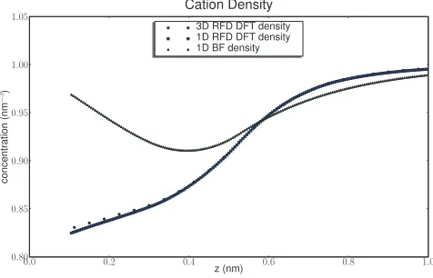
0.0 0.2 0.4 0.6 0.8 1.0

z (nm)

0.80 0.85 0.90 0.95 1.00 1.05

concentr

ation

(nm

−

3)

Cation Density

3D RFD DFT density 1D RFD DFT density 1D BF density

[image:7.612.317.555.559.712.2]

In Ref. 15, it is demonstrated that the BF version of DFT 关Eqs.共13兲and共14兲兴provides qualitatively incorrect densities when the surface charge is low, when compared with the

RFD functional 关Eqs. 共27兲–共34兲兴 and high resolution MC

simulation. We have successfully reproduced the 1D DFT and MC results with the 3D code, attesting to the correctness of our approach. Below, we discuss a representative simula-tion.

For our trial calculation, we examine a salt solution of univalent ions. The cation has radius 0.1 nm, the anion

0.2125 nm. Each species has a 1M bath concentration. The

simulation cell, 2⫻2⫻6 nm3, is periodic in each direction.

A hard, uncharged wall is placed a z= 0. We discretize the

density on a 21⫻21⫻161 grid. The results are insensitive to

the resolution in the transverse 共x−y兲 directions, but very

sensitive in the normal共z兲 direction. We verify the

homoge-neity of the solution acrossx−yplanes to machine precision.

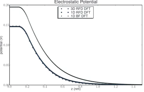
In Figs. 2 and3, we show the excellent match between 1D

and 3D DFT results, with MC results shown for comparison.

The mean electrostatic potential is shown in Fig.4, also with

good agreement.

The BF calculations are currently much more efficient than the RFD calculations, needing only 1.5 min compared

to more than a day to run since BF scales as O共NlogN兲,

whereas the RFD method scales as O共N2_{兲 and additional}

iterates are needed to obtain a converged reference density. However, the extra investment of time for RFD computations is necessary because the BF solution is qualitatively incor-rect compared to MC simulations.

VII. CONCLUSIONS AND FUTURE WORK

We have presented a full numerical strategy for solving the 3D equilibrium DFT system. The hard-sphere calculation accurately reproduces thermodynamic sum rules and agrees with prior MC simulation. Moreover, using the improved RFD electrostatic formulation due to Gillespieet al.,8we can accurately reproduce electrostatic behavior near a hard wall for species of differing radii. Thus, the DFT can now become a powerful tool for full 3D chemical simulation, accurately capturing both the energetic and entropic contributions to the solution.

There are also several avenues for improvement of the RFD algorithm and extension of the capabilities of the cur-rent code. The dominant cost of this algorithm is the calcu-lation of the reference density used to describe electrostatic screening. The current algorithm is very accurate, but

re-quiresO共N2兲work. Since the Fourier kernel is smooth and

has rapid decay, it should be possible to construct a multi-resolution analysis of it, resulting in a fast method for appli-cation. Moreover, the many FFTs performed at each Picard step could be replaced by unequally spaced FFTs or wavelet decompositions, which would allow adaptive refinement and increase the size of problems we can efficiently compute. The FFT and fast wavelet transform lend themselves readily to a scalable parallel implementations. In fact, it should also be possible to offload these transforms onto a multicore

co-processor, such as the Tesla 1060C GPU.28 This will make

large scale simulations of charged hard spheres accessible to working scientists even on a laptop or desktop computer. These algorithmic improvements are the focus of current re-search.

ACKNOWLEDGMENTS

This material is based upon work supported by, or in part by, the U. S. Army Research Laboratory and the U. S. Army Research Office under Contract No. W911NF-09-1-0488 共D.G. and M.G.K.兲. The work was also supported by NIH

Grant No, GM076013 共R.S.E.兲. M.G.K. was partially

sup-ported by the U.S. Department of Energy under Contract No.

DE-AC01-06CH11357. We thank Roland Roth and Dezső

Boda for helpful discussions.

APPENDIX A: CALCULATION OF THE BATH CHEMICAL POTENTIAL

Here we describe the formulas for the electrochemical potential in a homogeneous fluid. Here the DFT for hard

spheres uses a Percus–Yevick equation of state,29 and the

electrostatics is described using MSA.18,19 We follow the

treatment in Ref. 30. The bath chemical potential ␮i

bath

has two components, hard sphere and electrostatic,

0.0 0.2 0.4 0.6 0.8 1.0

z (nm)

0.95 1.00 1.05 1.10 1.15 1.20 1.25

concentr

ation

(nm

−

3)

Anion Density

[image:8.612.53.294.51.203.2]

3D RFD DFT density 1D RFD DFT density 1D BF density

FIG. 3. Comparing 1D and 3D DFT anion concentrations to MC simula-tions. The wall is uncharged, the cation concentration is 1M, and the ions are univalent. The 1D RFD DFT is shown with the blue squares, 3D RFD DFT with blue circles, and MC with green squares.

0.0 0.2 0.4 0.6 0.8 1.0 1.2 1.4

z (nm)

0.00 0.05 0.10 0.15 0.20

potential

(V)

Electrostatic Potential

3D RFD DFT 1D RFD DFT 1D BF DFT

[image:8.612.54.295.558.712.2]

␮i

bath

=␮i

HS,bath

+␮i

ES,bath

, 共A1兲

which are calculated thermodynamically,31

␮i

HS,bath

=kT

冉

− ln⌬+3␰2␴i+ 3␰1␴i

2

⌬ +

9␰₂2␴i2 2⌬2

+␲Pbath

HS_␴

i

3

6kT

冊

共A2兲

based upon the auxiliary variables, where␴iis the ion

diam-eter of speciesi,

␰n=

␲

6

兺

j

␳bathj ␴j n

n苸兵0, . . . ,3其, 共A3兲

⌬= 1 −␰3, 共A4兲

and the pressure due to hard-sphere interaction in the bath,

P_bathHS =6kT

␲

冉

␰0 ⌬ +

3␰₁␰₂

⌬2 +

3␰₂3

⌬3

冊

. 共A5兲

The calculation of␮i

HS,bath

as given above is straightforward, but␮i

ES,bath

, on the other hand, is dependent on an implicitly

defined parameter⌫, the MSA inverse screening length,

4⌫2= e

2

kT⑀⑀0

兺

j

␳j

bath

冉

zj−␩␴j2 1 +⌫␴j

冊

2

, 共A6兲

where␩represents the effects of nonuniform ionic diameters

␩= 1

⍀ ␲

2⌬

兺

j

␳j

bath_␴

jzj 1 +⌫␴j

共A7兲

and⍀is determined by

⍀= 1 + ␲

2⌬

兺

j

␳jbath␴3j 1 +⌫␴j

. 共A8兲

This implicit relationship is a quartic equation in ⌫, which

we solve using Newton’s method. We may then calculate the bath potential

␮iES,bath= −

e2

4␲⑀⑀0

冋

⌫zi

2

1 +⌫␴i +␩␴i

冉

2zi−␩␴i

2

1 +⌫␴i +␩␴i

2

3

冊

册

. 共A9兲

APPENDIX B: EVALUATION OF THE FOURIER TRANSFORM OF THE WEIGHTING FUNCTIONS

We must be careful to evaluate our analytic transforms at

the same kជ values, in the same order, as those computed

using the particular implementation of FFT we use. Given a

Ddimensional grid, the vector兵kd其which corresponds to the

vertex兵jd其of our Cartesian grid is given by

kd=

冦

2␲jd

Ndhd

, jdⱕ

Nd 2 , − 2␲共Nd−jd兲

Ndhd

, jd⬎

Nd

2 ,

冧

共B1兲

where Nd is the number of grid points in dimension d

苸兵x,y,z其 andhdis the grid spacingLd/共Nd− 1兲.

We begin with the calculation of␻ˆ_i2_,

␻ˆi2=

冕

0 2␲

d␾

冕

0

␲

d␪sin␪

冕

0

⬁

drr2_{␦共兩r兩−Ri兲e}−ıkជ·x_{ជ, 共B2兲}

=

冕

0 2␲

d␾

冕

0

␲

d␪sin␪Ri2e−ıRik

ជ·xˆ_{. 共B3兲}

We now choose a rotated coordinate system共the prime

sys-tem兲in whichkជpoints purely in thez

⬘

direction, in order to take advantage of the rotational symmetry of the problem. In the new coordinate system,

␻ˆi2=

冕

0 2␲

d␾

⬘

冕

0

␲

d␪

⬘

sin␪

⬘

Ri2e−ıRikz⬘cos␪⬘, 共B4兲

=2␲Ri2

冕

0

␲

d␪

⬘

sin␪

⬘

共cos共Rikz

⬘

cos␪

⬘

兲

−ısin共Rikz

⬘

cos␪

⬘

兲兲, 共B5兲

=4␲Risin共Rikz

⬘

兲

kz

⬘

, 共B6兲

which, in the original coordinate system, is

␻ˆ_i2=4␲Risin共Ri兩kជ兩兲

兩kជ兩 . 共B7兲

From Eq.共8兲, we also have

␻ˆ_i0=sin共Ri兩kជ兩兲

Ri兩kជ兩 ␻ˆi 1

=sin共Ri兩kជ兩兲

兩kជ兩 . 共B8兲

Recognizing that the theta function can be obtained as the integral of a delta function, we have

␻ˆ_i3=

冕

0

R_i

dr␻ˆ_i2兩R

i=r, 共B9兲

=4␲ 兩kជ兩

冕

0

R_i

drrsin共r兩kជ兩兲, 共B10兲

=4␲

兩kជ兩3共sin共Ri兩kជ兩兲−Ri兩kជ兩cos共Ri兩kជ兩兲兲. 共B11兲

Following a similar procedure as in the ␻ˆ_i2 _{calculation, but}

keeping track of the vector nature of␻V1 _and␻V2_,

␻ˆ_iV2=

冕

0 2␲

d␾

⬘

冕

0

␲

d␪

⬘

sin␪

⬘

Ri

2

e−ıRikz⬘cos␪xˆ_, 共B12兲

=− 2␲ıRi

冕

0

␲

d␪

⬘

sin␪

⬘

cos␪

⬘

sin共Rikz

⬘

cos␪

⬘

兲kˆz

⬘

,

=− 4␲ı

兩kជ兩2 共sin共Ri兩kជ兩兲−Ri兩kជ兩cos共Ri兩kជ兩兲兲kˆ. 共B14兲

The preceding expressions for ␻ˆ_i␣ may be evaluated at 兩kជ兩

= 0, but care must be taken when calculating the limit.

lim

兩kជ_兩→0

␻ˆ_i0= lim

兩kជ_兩→0

sin共Ri兩kជ兩兲

Ri兩kជ兩 = 1,

lim

兩kជ兩→0

␻ˆ_i1=Ri,

lim

兩kជ兩→0

␻ˆ_i2_{= 4␲R}

i

2_,

lim

兩kជ兩→0

␻ˆi3= lim

兩kជ兩→0

4␲

兩kជ兩3

冉冉

Ri兩kជ兩−

共Ri兩kជ兩兲3

6

冊

−Ri兩kជ兩

冉

1 −共Ri兩kជ兩兲

2

2

冊冊

,

=4 3␲Ri

3_,

lim

兩kជ兩→0

␻ˆi

V1_{= 0,}

lim

兩kជ兩→0

␻ˆ_iV2= 0.

It should be noted these are the limits one would expect since in the兩kជ兩= 0 case we are simply integrating either a spherical delta or step function over all space, thereby recovering sur-face area and volume expressions for a sphere.

APPENDIX C: DIRECTIONAL AVERAGE BOUND

We can bound the directional average of the density over a sphere in terms of the unweighted average, and thus we can bound the ratio

兩nV2共x兲兩2

兩n2共x兲兩2 共C1兲

in the calculation of ⌽共n兲 from Eq.共10兲. We let ␯共␪,␾兲 be

the unit vector at the surface of the sphere in the 共␪,␾兲

direction. Using Fubini’s theorem and the Cauchy–Schwarz inequality, we have

nV22共x兲=

兺

ij

冕

S2

␯共␪,␾兲␳i共x+r兲d⍀

·

冕

S2

␯共␪

⬘

,␾

⬘

兲␳j共x+r

⬘

兲d⍀

⬘

, 共C2兲

=

兺

ij

冕

S2⫻S2

␯共␪,␾兲·␯共␪

⬘

,␾

⬘

兲

⫻␳i共x+r兲␳j共x+r

⬘

兲d⍀d⍀

⬘

, 共C3兲

ⱕ

兺

ij

冕

S2⫻S2

兩␯共␪,␾兲·␯共␪

⬘

,␾

⬘

兲兩兩␳i共x+r兲

⫻␳j共x+r

⬘

兲兩d⍀d⍀

⬘

, 共C4兲

ⱕ

兺

ij

冕

S2⫻S2

兩␯共␪,␾兲兩兩␯共␪

⬘

,␾

⬘

兲兩␳i共x+r兲

⫻␳j共x+r

⬘

兲d⍀d⍀

⬘

, 共C5兲

ⱕ

兺

ij

冕

S2_⫻S2

␳i共x+r兲␳j共x+r

⬘

兲d⍀d⍀

⬘

, 共C6兲

=

兺

ij

冕

S2

␳i共x+r兲d⍀

冕

S2

␳j共x+r

⬘

兲d⍀

⬘

, 共C7兲

=n₂2共x兲, 共C8兲

so that

兩nV2_共x兲兩2

兩n2共x兲兩2 ⱕ1. 共C9兲

1_{R. Evans,Adv. Phys. 28, 143共1979兲.} 2_{J. Wu,AIChE J. 52, 1169共2006兲.}

3_{D. Gillespie, L. Xu, Y. Wang, and G. Meissner,J. Phys. Chem. B 109,}

15598共2005兲.

4_{D. Gillespie,Biophys. J. 94, 1169共2008兲.}

5_{R. Roth, R. Evans, A. Lang, and G. Kahl,J. Phys.: Condens. Matter 14,}

12063共2002兲.

6_{Y.-X. Yu and J. Wu,J. Chem. Phys. 117, 10156共2002兲.}

7_{H. Hansen-Goos and R. Roth, J. Phys.: Condens. Matter 18, 8413} 共2006兲.

8_{D. Gillespie, W. Nonner, and R. S. Eisenberg,J. Phys.: Condens. Matter}

14, 12129共2002兲.

9_{D. Gillespie, W. Nonner, and R. S. Eisenberg,Phys. Rev. E 68, 031503} 共2003兲.

10_{Y.-X. Yu and J. Wu,J. Chem. Phys. 116, 7094共2002兲.} 11_{Y. Rosenfeld,Phys. Rev. Lett. 63, 980共1989兲.} 12_{Y. Rosenfeld,J. Chem. Phys. 98, 8126共1993兲.}

13_{R. Evans,Fundamentals of Inhomogeneous Fluids共CRC, Boca Raton,}

1992兲, pp. 85–176.

14_{URL:https://software.sandia.gov/DFTfluids/index.html.}

15_{D. Gillespie, M. Valiskó, and D. Boda,J. Phys.: Condens. Matter 17,}

6609共2005兲.

16_{Y. Rosenfeld, M. Schmidt, H. Löwen, and P. Tarazona,Phys. Rev. E 55,}

4245共1997兲.

17_{L. Blum and Y. Rosenfeld,J. Stat. Phys. 63, 1177共1991兲.}

18_{E. Waisman and J. L. Lebowitz,J. Chem. Phys. 56, 3086共1972兲, URL:}

http://link.aip.org/link/?JCP/56/3086/1.

19_{L. Blum,Mol. Phys. 30, 1529共1975兲.}

20_{URL:http://en.wikipedia.org/wiki/Heaviside_step_function.}

21_{S. Balay, K. Buschelman, V. Eijkhout, W. D. Gropp, D. Kaushik, M. G.}

Knepley, L. C. McInnes, B. F. Smith, and H. Zhang, Technical Report ANL-95/11-Revision 3.0.0, Argonne National Laboratory, 2009, URL: http://www.mcs.anl.gov/petsc/docs.

22_{M. Frigo and S. G. Johnson,Proc. IEEE 93, 216共2005兲 共special issue on}

“Program Generation, Optimization, and Platform Adaptation”兲.

23_{R. Roth,J. Phys.: Condens. Matter 22, 063102共2010兲.}

24_{Y. Saad and M. H. Schultz, SIAM共Soc. Ind. Appl. Math.兲J. Sci. Stat.}

Comput. 7, 856共1986兲.

26_{J. Goodman and A. D. Sokal,Phys. Rev. D 40, 2035共1989兲.} 27_{D. Frenkel,Proc. Natl. Acad. Sci. U.S.A. 101, 17571共2004兲.} 28_{URL:http://www.nvidia.com/object/product_tesla_c1060_us.html.} 29_{J. L. Lebowitz,Phys. Rev. 133, A895共1964兲.}

30_{W. Nonner, L. Catacuzzeno, and B. Eisenberg,Biophys. J. 79, 1976} 共2000兲.

31_{W. Nonner, D. Gillespie, D. Henderson, and R. Eisenberg,J. Phys. Chem.}