Manuscript accepted for publication in International Journal of Speech Technology, February 5, 2001
Improved Data Modeling for Text-Dependent Speaker
Recognition Using Sub-Band Processing
R.A. Finan , R.I. Damper†and A.T. Sapeluk
School of Engineering University of Abertay Dundee
Scotland DD1 1HG Emails:
r.a.finan|a.t.sapeluk @tay.ac.uk
†Image, Speech and Intelligent Systems (ISIS) Research Group
Department of Electronics and Computer Science University of Southampton
Hants SO17 1BJ, UK Email:rid@ecs.soton.ac.uk
Abstract
A growing body of recent work documents the potential benefits of sub-band processing over wideband pro-cessing in automatic speech recognition and, less usually, speaker recognition. It is often found that the sub-band approach delivers performance improvements (especially in the presence of noise), but not always so. This raises the question of precisely when and how sub-band processing might be advantageous, which is difficult to answer because there is as yet only a rudimentary theoretical framework guiding this work. We de-scribe a simple sub-band speaker recognition system designed to facilitate experimentation aimed at increasing understanding of the approach. This splits the time-domain speech signal into 16 sub-bands using a bank of second-order filters spaced on the psychophysical mel scale. Each sub-band has its own separate cepstral-based recognition system, the outputs of which are combined using the sum rule to produce a final decision. We find that sub-band processing leads to worthwhile reductions in both the verification and identification error rates relative to the wideband system, decreasing the identification error rate from 3.33% to 0.56% and equal error rate for verification by approximately 50% for clean speech. The hypothesis is advanced that, unlike the wide-band system, sub-wide-band processing effectively constrains the free parameters of the speaker models to be more uniformly deployed across frequency: as such, it offers a practical solution to the bias/variance dilemma of data modeling. Much remains to be done to explore fully the new paradigm of sub-band processing. Accordingly, several avenues for future work are identified. In particular, we aim to explore the hypothesis of a practical solution to the bias/variance dilemma in more depth.
1
Introduction
it as “the Stewart-Fletcher multiindependent channel model” (p. 572). He further characterizes the approach as “across-time” rather than the more usual “across-frequency” processing (p. 575) typified by template matching in automatic speech recognition. In this paper, we will use the term sub-band processing. The positive benefits of this new approach to speech recognition are starting to be investigated and reported (Bourlard and Dupont 1996; Hermansky, Tibrewala, and Pavel 1996; Tibrewala and Hermansky 1997; Hermansky and Sharma 1998; Okawa, Bocchieri, and Potamianos 1998; Morris, Hagen, and Bourlard 1999). There is every reason to expect that sub-band processing might also profitably be applied to speaker recognition, improving prospects for real-world applications.
There are, however, several practical issues and choices which have not yet been fully studied and resolved:
The number, location and detailed shape of the frequency bands must be chosen.
Some knowledge of which bands contain the most speaker-dependent information is required. The scores from these bands might then be emphasized/weighted to improve recognition.
The features to be used for recognition must be decided, bearing in mind that features designed for speech recognition may not be suitable for speaker recognition (Furui 1997). (It is also possible that features which are appropriate for wideband speaker recognition are less so for sub-band processing.)
The rule for combination of individual outputs must be decided. How, for instance, might we define a rule which implements the Fletcher-Allen principle, i.e., such that the global error rate is equal to the product of the individual, sub-band error rates? Further, the Fletcher-Allen assumption of independent channels is itself problematic (Steeneken and Houtgast 1999).
The point in the system at which the scores are combined must be decided. Depending on whether the tests are text-dependent or text-independent, and the type of recognition system used, combination could be at the end of a frame, phoneme, syllable, word or sentence.
To date, relatively few workers have studied this problem in the context of speaker recognition. In the con-ference literature, Besacier and Bonastre (1997), Auckenthaler and Mason (1997), Sivakumaran, Ariyaeeinia, Hewitt, and Malcolm (1998) and Sivakumaran, Ariyaeeinia, and Hewitt (1998) have all presented empirical results which confirm that worthwhile performance advantages can be gained from sub-band processing in this application. Taken together, however, these prior works do not cover anything like the full range of imple-mentation options, so that many of the aforementioned questions remain open. Further, there is still only a rudimentary understanding of sub-band processing – and precisely how it delivers performance improvements – from a theoretical perspective. The aim of this paper is to describe a simple sub-band speaker recognition system designed to facilitate empirical exploration of (at least some of) these questions, and to report some new empirical results, but also to fit these into an emerging theoretical framework of data modeling, classifier com-bination and information fusion. At this stage, and in order to provide a baseline for future work, we restrict ourselves to the study of clean speech.
The remainder of this paper is structured as follows. In Section 2, we give a brief statement of the speaker recognition problem, and detail the sub-problem of text-dependent recognition which is the focus of the present work. Section 3 presents a review of previous work in sub-band speech processing, emphasizing speaker recognition. Section 4 describes prior work with a wideband system which forms the basis of the particular sub-band system studied here, which is outlined in Section 5. Next, Section 6 details the several different ways of combining scores which were investigated (although all were based on the sum rule) and presents the corresponding results which indicate a significant improvement due to sub-band processing. In Section 7, we develop the hypothesis that this improvement occurs because the data modeling problem (here, linear prediction followed by vector quantization) is more tightly constrained relative to the wideband case. Finally, Section 8 discusses our findings and interprets them in a data engineering framework before concluding.
2
The Speaker Recognition Problem
aim is to determine if a given utterance was produced by the claimed speaker. This is most directly done by testing the utterance against the model of the claimed speaker, comparing the score to a threshold, and deciding on the basis of this comparison whether or not to accept the claimant. In identification, the aim is to determine which speaker from among a known group produced the utterance. In this case, the test utterance is scored against all possible speaker models, and that with the best score determines the speaker identity. Of the two tasks, identification is generally accepted to be the harder, especially for large speaker populations (Doddington 1985, p. 1660).
In text-independent recognition, there are no limits on the vocabulary employed by speakers. This is in contrast to text-dependent recognition, where the presented utterance must be from a set of predetermined words or phrases. As text-dependent recognition only models the speaker for a limited set of phonemes in a fixed context, it generally achieves higher recognition rates than text-independent recognition, which must model a speaker for a variety of phonemes and contexts. In this paper, we apply sub-band processing both to verification and identification in the text-dependent case. Text-dependent recognition was chosen because of its more obvious applicability, especially for verification (Doddington 1985, p. 1660).
Since identification is simply a matter of selecting among speakers, typically using a minimum distance decision rule, performance is easily quantified by a single measure. There are only two possible outcomes – correct or incorrect – so that the identification error (IE) fully specifies the situation. Things are a little more complicated with verification where the system has to accept or reject a claimed speaker identity in the face of potential impersonation. Hence, there are four possible outcomes, of which two – false acceptance (FA) and false rejection (FR) – are errors. Thus, some decision threshold must be set which effects a balance between the two types of error. While it is possible to devise a general cost function which does this, we do not know the relative costs of the two types of error here. Hence, they are simply assumed to be equal and the threshold is set to equalize the FA and FR rates. The performance measure employed is thus the equal error rate (EER).
3
Previous Work on Sub-Band Processing
Most current speaker recognition systems use wideband processing, whereby the whole frequency range is covered by a single recognition system. Typically, either mel-scale cepstral coefficients or linear prediction cepstral coefficients (LPCCs) are used as the feature set. In sub-band processing, the speech signal is split into band-limited channels. Each has its own recognition system, and the final score for an utterance is calculated by combining the individual scores.
In early work, Bourlard and Dupont (1996) investigated sub-band processing for automatic speech recogni-tion using a hidden Markov model (HMM) system, with the intenrecogni-tion of improving robustness in noise. Several parameters were investigated, including the number and location of the bands, the feature set and the scheme for combining individual scores. They found that 4 to 5 bands performed well, but that further investigation was warranted before any firm conclusions could be drawn. With regard to the feature set, modeling the filter-bank outputs in terms of LPCCs (with cepstral mean subtraction) was more successful than using critical band energies (0.5% error rate versus 2.0% using four sub-bands).
Combination strategies were based on weighted summations. This makes intuitive sense, as the outputs of their recognizers were estimates of log-likelihoods. As well as unweighted combination, they also studied weighting by the (normalized) phoneme-level recognition rates in each band and by (normalized) signal-to-noise ratios in each band. Because “it is often argued that the recombination mechanism should be non-linear” (p. 427), Bourlard and Dupont also used a multilayer perceptron (MLP) trained to estimate posterior probabilities of speech units (given the log-likelihoods of all sub-bands and all speech units) for score combi-nation. Of these, the MLP gave the best results but the other weighting schemes also performed well compared to the wideband system. Although sub-band processing gave better results than wideband processing when narrow-band noise was present, it gave poorer recognition rates than a wideband system using J-RASTA noise cancellation (Hermansky and Morgan 1994). However, using J-RASTA first, followed by sub-band processing, led to lower error rates than for the wideband system (9.1% versus 12.1%).
which may be irrelevant to a speech recognition task” (p. 3). With colleagues, Hermansky has pursued this idea in a series of publications (Hermansky, Tibrewala, and Pavel 1996; Tibrewala and Hermansky 1997; Herman-sky and Sharma 1998). One development has been the full combination method (HermanHerman-sky 1998; Morris, Hagen, and Bourlard 1999) whereby the assumption of independence between channels can be avoided if a separate neural/HMM recognizer is trained on each possible combination of sub-bands. This idealization is computationally prohibitive but useful, practical approximations are presented by Morris, Hagen, and Bourlard. Turning now to speaker recognition, Besacier and Bonastre (1997) applied sub-band processing to text-independent identification with clean speech. Tests were carried out on all 630 speakers of the TIMIT database, using the phonetically-compact (SX) sentences for training and the dialect (SA) and phonetically-rich (SI) sentences for testing. They used spectral energies in sub-bands as the basic feature set. A total of 24 “channels” was created using “mel-scale triangular filterbank coefficients” (p. 196) calculated from the Winograd Fourier transform power spectrum and expressed “in logarithmic scale” (p. 197). (Terminology here is potentially confusing. We use channel as a synonym for sub-band, but Besacier and Bonastre’s sub-band is a combination of channels.) Channels were grouped in various ways to produce “sub-bands” in their terms. Recognition was based on second-order statistical measures (Bimbot and Mathan 1994) with a 1-nearest neighbor decision rule. The combination strategy was to compute the arithmetic mean of the separate sub-band distances, after 3 seconds and after 6 seconds of speech.
Initially, channels were grouped in overlapping sets of four to create 21 sub-bands as follows. Sub-band 1 encompassed channels 1–4, sub-band 2 covered channels 2–5, etc. Besacier and Bonastre found that certain sub-bands contained more speaker-specific information than others: in particular, the low-frequency region below 600 Hz and the high-frequency region above 2 kHz. This helps to explain the poorer performance rates for telephone-quality speech (e.g., Naik, Netsch, and Doddington 1989), where some of these critical high and low frequency regions are absent.
A variety of architectures was studied in which different numbers of sub-bands were included/excluded. (Unfortunately, Besacier and Bonastre do not report comparisons with a single, wideband system.) They found that sub-bands formed from consecutive channels (1, 2, 3, . . . ) gave far better results than those formed from “crisscrossed” channels (1, 3, 5, . . . ). Hence, they write, “the correlations between close channels are important when second-order statistical measures are used” (p. 201). They also found that performance decreased when the sub-bands became smaller (in terms of number of channels) and more numerous. This was felt to reflect the concomitant reduction in the number of parameters used to model a speaker.
A similar approach has also been described by Auckenthaler and Mason (1997). They used spectral analysis to generate 32 bins (cf., Besacier and Bonastre’s “channels”), which were grouped together in varying sizes to form sub-bands. Using a warping function to create approximately equal identification error rates for each band, they found that for text-dependent speaker identification experiments, sub-band processing gave comparable results to wideband processing.
Sivakumaran, Ariyaeeinia, Hewitt, and Malcolm (1998) and Sivakumaran, Ariyaeeinia, and Hewitt (1998) concentrated on the weighting scheme to be used in conjunction with the sum rule of score combination in speaker verification. They propose the use of “dynamic” weights, computed from competing speaker models. Various verification systems were trained on 10 repetitions of the ten digits from 20 male speakers in the Mil-lar database (see next section). Then, using four (overlapping) mel-spaced bands and dynamic combination weights, an equal error rate (EER) of just under 10% was achieved for 15 unseen repetitions of the ten digits from the same 20 speakers. The corresponding figure for a full-band HMM system was approximately 15%. The sub-band system performed far better with added noise, however. One-third of the utterances was con-taminated with narrowband (0–600 Hz) noise. At 0 dB signal-to-noise ratio, the full-band system gave an EER of approximately 29% relative to just over 10% for the sub-band system. This confirms the effectiveness of de-emphasizing regions of the spectrum contaminated by noise.
4
Prior Work with Wideband System
4.1
Database
The British Telecom Millar database was specifically designed and recorded for text-dependent speaker recog-nition studies. It consists of 46 male and 14 female native English speakers repeating the words one to nine, zero, nought and oh 25 times each. The database was recorded in five sessions spaced over three months. At each session, speakers were prompted visually to say the words in a random order. Recordings were made in a quiet environment using a high-quality microphone. The speech was digitized at a sampling rate of 20 kHz with a 16-bit A/D converter. As well as the 20 kHz recording, the database was also made available at an 8 kHz sampling rate. In this latter version, the speech has been bandpassed to 3.6 kHz with a third-order Butterworth filter and then downsampled. Only the 8 kHz version was used in the experiments reported here.
4.2
Implementation of the wideband system
The feature set used for recognition consisted of cepstral coefficients derived from linear prediction analysis (Markel and Gray 1976; Picone 1993; Schroeder 1999). Cepstral coefficients are well recognized as one of the best speech representations for both speaker and speech recognition (Furui 1997). Using an analysis frame of 20 ms, Hamming windowed and overlapping by 50%, 12th order linear predictor coefficients were obtained. These were then used to create cepstral coefficients via the recursion described by Atal (1974).
Speaker models were produced by vector quantization (VQ) with a codebook size (determined empirically, see Finan 1998) of 32. VQ has been used extensively for both text-dependent and text-independent speaker recognition (Rosenberg and Soong 1987; Booth, Barlow, and Watson 1993; Yu, Mason, and Oglesby 1995). It is a data reduction technique in which similar vectors are grouped together and represented by their centroid. The grouping is repeated iteratively until the distance (see below) between each vector and its group centroid has been minimized. These centroids make up the codebook which models the data, and their number will determine the accuracy of the modeling. The standard LBG algorithm (Linde, Buzo, and Gray 1980) was applied to calculate the centers.
Distances between vectors j and k (codebook centers or test utterance frames) were calculated using the ‘city block’ measure:
d j k
12
i 1
ci j cik
where ci j is the i th cepstral coefficient of vector j , similarly cik for vector k. (As usual, c0was discarded.)
When testing an utterance against a VQ speaker model, the utterance and model are first optimally aligned by dynamic time warping. The city-block distance is then summed over the total number of aligned frames, i.e., along the optimal path. This sum was then averaged over the number of aligned frames to give the final score. The decision rule was simply to select the speaker providing the best scoring sequence of codebook vectors.
4.3
Impostor cohort normalization
Verification recognition rates may be improved through the use of score normalization (Furui 1997). For some of the tests reported here, impostor cohort normalization (ICN) was used. The ICN derived scores have better equal error rates than the un-normalized scores (Finan et al. 1997).
ICN is based on the fact that the genuine speaker score remains fairly stable relative to the impostor score distribution, although the impostor score distribution itself may vary considerably (Li and Porter 1988). The scores from the impostor models are used to normalize the genuine speaker model score. So each utterance is presented to the genuine speaker model and a limited set of impostor models. The genuine speaker score is then normalized by the mean and standard deviation of the impostor scores as follows:
SICN
Sgen mcoh
S Dcoh
(1) where SICNis the normalized score, Sgen is the original genuine speaker model score and mcoh and S Dcohare
IE (%) FA (%) FR (%) EER (%)
All 31 speakers 4.73 5.95 5.03 5.92
12 speakers 3.33 10.10 8.89 10.00
Table 1: Comparison of the identification and verification results for the full database of 31 male speakers and restricted database of 12 male speakers for the word seven with the wideband system.
Note that this normalization procedure somewhat blurs the traditional distinction between identification and verification. ICN works by using identification: it looks at the genuine speaker score in relation to those for other speakers. That is, the scores from the other models are used to normalize the test against the genuine speaker model. If the utterance is from the genuine speaker, this should get the lowest score (as in identifica-tion).
In the experiments carried out here, the six most effective impostors were selected to form the cohort (Finan 1998). Then the best five impostors were selected for a speaker’s cohort unless that speaker was also a member of the cohort, in which case the sixth impostor was used. Thus, no speaker was part of his/her own cohort.
A related technique is to employ ‘world’ or ‘background’ models (e.g., Carey and Parris 1992; Matsui and Furui 1995; Rosenberg and Parthasarathy 1996; Reynolds 1997) – either a composite constructed for a subset of speakers or one per background speaker. Verification is then on the basis of the likelihood ratio between the score for the claimed speaker’s model and that for the composite or the average for the background speakers, as appropriate. This obviates the need to set a decision threshold. With the system described here, this approach did not work as well as cohort normalization (Finan 1998).
4.4
Results of wideband recognition
In previous work, 31 male speakers of the same age group (20–29 years) saying the words one to nine and zero were used (Finan et al. 1997). Male speakers alone were used as this represents a generally harder identification problem than using a mixed male/female set. A selection of the speakers (rather than the full set of 46) was used because of the computational complexity of the software simulation. From these experiments, it became clear that some speakers were more problematic than others. These poorer speakers, often referred to as goats – from the adage “sorting the sheep from the goats” (Doddington, Liggett, Martin, Przybocki, and Reynolds 1998) – are responsible for most of the errors encountered (Thompson and Mason 1994). For the sub-band experiments reported shortly, a subset of 12 of the male speakers saying the word seven was chosen: 8 problem speakers and 4 others. A smaller set of speakers (12 rather than 31) was used because of the much increased computational complexity of sub-band relative to wideband processing. The 8 poor speakers were those who performed worst in the earlier tests. The other 4 were chosen at random. Recordings from the first two sessions (i.e., 10 repetitions of seven) were used for training and those from the remaining three sessions (15 repetitions) were used for testing.
Test
Utterance
Filter 1
Filter 2
Filter 3
Filter 15
Filter 16
Recogniser 1
Recogniser 2
Recogniser 3
Recogniser 15
Recogniser 16
Global Score LPCC
LPCC
LPCC
LPCC
LPCC
Score Combination
[image:7.612.75.546.37.161.2]
Figure 1: Block diagram of the LPCC-based sub-band processing system. Sub-band Center Frequency (Hz) Bandwidth (Hz)
1 83 101
2 176 102
3 280 106
4 396 111
5 526 119
6 671 130
7 833 144
8 1015 164
9 1218 188
10 1446 218
11 1700 254
12 1985 298
13 2303 351
14 2659 415
15 3057 490
[image:7.612.182.419.208.420.2]16 3502 580
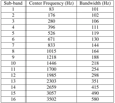
Table 2: Center frequencies and bandwidths for the 16 sub-bands.
5
Implementation of Sub-Band Processing
Figure 1 depicts a block diagram of the sub-band speaker recognition system. Component parts will be de-scribed and discussed in turn. No claim is made that this system is state-of-the-art. Rather, it is intended as a simple yet adequate vehicle for the study of the sub-band approach – allowing a range of implementation details to be varied and assessed.
5.1
Filterbank
The wideband speech signal is split into 16 bands, equally spaced in frequency according to the mel scale – a non-linear scale based on the human auditory system (Zwicker and Terhardt 1980). Such a scale was used by Besacier and Bonastre (1997), but not by Bourlard and Dupont (1996) who used fewer sub-bands. The choice of 16 bands may not be optimal, but was chosen in light of Allen’s (1994) comment: “It has been reported . . . that 10 bands is too few, and 30 bands gives no improvement in accuracy over 20” (p. 572). The center frequencies and bandwidths of the 16 filters are given in Table 2.
0 500 1000 1500 2000 2500 3000 3500 4000 −60
−50 −40 −30 −20 −10 0
Frequency
[image:8.612.140.461.39.288.2]dB
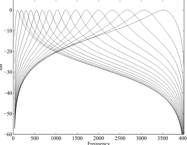
Figure 2: Characteristics of the 16 bandpass filters.
time domain by direct calculation from the difference (recurrence) equation. The advantage of IIR filters is their ease of design and implementation; the disadvantage is that they have a non-linear phase response. The effect of this on the results of recognition remain to be ascertained. The filter characteristics are depicted in Figure 2. Note that in this simple scheme, the degree of overlap of adjacent filter skirts is uncontrolled, although the point of crossover is never too far from 3 dB. As the filters are only second-order, there is considerable overlap
at the level of 10 dB, for instance. However, the higher the order of the filter, the more poles of the linear
prediction (LP) analysis would be required to model the filter rather than the speech. Thus, it was a deliberate decision to use low order filters.
5.2
Individual recognizers
The individual recognizers were identical to the wideband system described by Finan et al. (1997) and above (Section 4.2), as were the training and test conditions.
5.3
Score combination
Score combination is a particular, restricted instance of a data fusion problem. As stated above, initial work in sub-band speech processing (Bourlard and Dupont 1996) used weighted summation to combine scores. This was intuitively satisfactory, because the individual scores were estimates of log-likelihoods and this formulation has subsequently been improved in the so-called ‘full-combination’ approach (Hermansky, Tibrewala, and Pavel 1996; Hermansky 1998; Morris, Hagen, and Bourlard 1999). However, other work (e.g., Sivakumaran, Ariyaeeinia, and Hewitt 1998) has sometimes retained this formulation even though the scores were not log-probability-like. In our case, scores are city block distances, so it is not immediately clear that weighted summation is the best combination technique.
“there is presently inadequate understanding why some combination schemes are better than others and in what circumstances” (p. 226). Thus, Kittler et al. outline a number of possible rules of combination – viz. product, sum, max, min, median and majority vote rules – and the assumptions behind them as well as relations between them. These rules were then compared empirically for performance on the representative pattern recognition problems of person identification (combining two face views and voice) and handwritten digit recognition (combining four different classifier designs). It was found that the sum rule performed consistently well. On the person identification task, it achieved an EER of 0.7% relative to 1.2% for the next best (median) rule and 1.4% for the best single modality (speech). On the handwritten digit task, it gave a classification rate of 98.05%, which was the second-best figure after the median rule (98.19%). These compare with 94.77% for the best individual (HMM) recognizer.
Kittler et al. express surprise that the sum rule produces “the most reliable decisions” given that it “has been developed under the strongest assumptions” (p. 235). Specifically, the statistical assumptions are conditional independence of the respective representations used by the individual classifiers and highly ambiguous classes (such that observations enhance the a priori probabilities only slightly). It is shown theoretically that the sum rule is much less sensitive to estimation errors than the product rule, a fact which is consistent with the experimental findings and almost certainly explains the “surprising” superiority of the sum rule. For these reasons, we have chosen to use a sum rule here, but recognize that future work should be directed at a more thorough investigation of different score combination methods in sub-band speaker recognition.
6
Results of Sub-Band Recognition
In this work, the number of sub-bands and their center frequencies were fixed. Also, as detailed in Section 5.3, we use the sum rule of combination – both with and without weighting – to produce the final score. The most straightforward method, however, is unweighted summation. This was the only combination strategy used by Besacier and Bonastre (1997) and one of several tested by Bourlard and Dupont (1996).
6.1
Unweighted combination
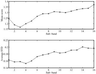
The average verification scores (computed as in equation 1) for the test data and their average standard deviation are depicted for each of the 16 bands in Figure 3. As the scores are all quite similar, it seems that no particular band will dominate the (unweighted) sum. The results using the simple, unweighted sum rule of combination are shown in Table 3 (bottom row). Compared with the performance of the wideband system (top row of Table 3 and bottom row of Table 1), it is clear that sub-band processing leads to a consistent improvement for all the performance measures. For instance, identification error falls from 3.33% to 0.56% (a decrease from 6 misclassified utterances to just 1). As the identification error is also important to the score normalization (see Section 4.3 above), the ICN equal error rate reflects this with a drop from 3.66% for the wideband case to 1.39% for the sub-band case.
Since only two outcomes are possible for identification – either the speaker is correct or not – the sampling distribution of these errors is binomial. Hence, we can use a binomial test (Siegel 1956, pp. 36–38) to deter-mine the significance of the above differences. The probability of observing k or fewer errors in n trials when sampling from a binomial distribution with mean error probability e is:
pk
k
r 0
nCrer
1 e
n r
(2) wherenCr is the binomial coefficient. For the case of identification error, n = 180 utterances, e 0101, and
k 1. This yields p1 001613 as the probability that one or fewer identification errors could have been
obtained by chance if there were no difference between the wideband and sub-band distributions, i.e., the dif-ference is significant at the 2% level. Hence, sub-band processing leads to significantly improved identification performance in this case.
2 4 6 8 10 12 14 16 1.15
1.2 1.25 1.3 1.35 1.4
Sub−band
Mean score
2 4 6 8 10 12 14 16
0.14 0.16 0.18 0.2 0.22
Sub−band
[image:10.612.139.463.97.349.2]Average STD
Figure 3: Mean verification scores and their standard deviations for each sub-band.
Un-normalized ICN
IE (%) FA (%) FR (%) EER (%) FA (%) FR (%) EER (%)
Wideband 3.33 10.1 8.89 10.0 3.84 1.67 3.66
Sub-band 0.56 5.30 4.00 5.19 1.52 0.0 1.39
[image:10.612.114.484.497.564.2]Significance NS NS NS
Table 3: Comparison of the wideband and sub-band processing results using the unweighted sum rule. (KEY:
– highly significant at 2% level; – significant at 5% level; – marginally significant at 10% level; NS
1 2 3 4 5 6 7 8 9 10 11 0.8
0.9 1 1.1 1.2 1.3 1.4 1.5
Speaker model
[image:11.612.146.460.39.291.2]Utterance score
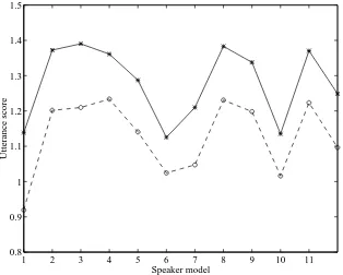
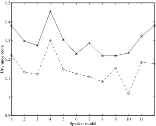
Figure 4: Example showing that sub-band processing improves identification of Speaker 1. The self-test score is the lowest obtained with sub-band processing, so that Speaker 1 is correctly identified. The wideband system erroneously identifies Speaker 6, and Speaker 10 also has a lower score than Speaker 1 (‘*’ = wideband scores, ‘o’ = average sub-band scores).
integer,k . In the un-normalized case, there are respectively highly significant and significant reductions in FA
( p 000175) and EER ( p 002450) due to sub-band processing. The reduction in FR is of the same order
(approximately 50%) but is far from significance ( p 06096) because of the much smaller number of
genuine-speaker tests (15 as opposed to 165 impostor tests). When impostor cohort normalization is used, however, the results are less impressive, reflected in marginal significance for EER only ( p 0100). Presumably, ICN
effectively removes some of the potential for achieving gains through sub-band processing. It seems likely that testing with a larger number of utterances would have produced more obviously significant improvements for ICN, but the considerable time necessary to simulate the sub-band system precluded this in practice.
Particular illustrations of the advantages of sub-band processing in reducing identification error rate relative to the wideband system are given in Figures 4 and 5. The figures show the identification scores for two utterances using both wideband and sub-band processing when test utterances were presented to all 12 speaker models. (As the task is identification, the model with the lowest score determined the speaker.) In the wideband case, the utterance from Speaker 1 is attributed to Speaker 6 (Fig. 4), and in the second example the utterance from Speaker 10 is attributed to Speaker 8 (Fig. 5). However, using an unweighted sum combination strategy, the sub-band system attributes the utterances to the correct speakers. In both examples, the utterance still scores best against the same impostor model, but the score against the genuine speaker model is even lower. The direct implication is that sub-band processing produces a better genuine speaker model in these cases.
6.2
Weighted combination
1 2 3 4 5 6 7 8 9 10 11 0.9
1 1.1 1.2 1.3 1.4 1.5
Speaker model
[image:12.612.145.458.38.291.2]Utterance score
Figure 5: Further example showing how sub-band processing improves identification of Speaker 10 compared to the wideband system which erroneously identifies Speaker 8 (‘*’ = wideband scores, ‘o’ = average sub-band scores).
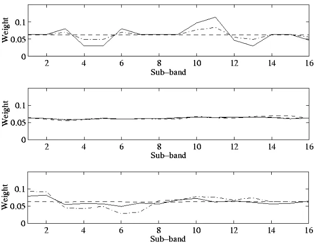
In both cases, the weight could be determined in three ways: one a priori and the other two a posteriori. With a priori weightings, only the results based on the training data can be used. This works for the EER, but the identification error rate on the training data is zero, so it could not be used for (1) above. The two a posteriori methods involve the test data only and the test data combined with the training data, respectively. Figure 6 shows the variation of identification error and equal error rate across the 16 bands using each of the three possible evaluation methods: training set only, test set only and combination of training and test sets. These measures of speaker recognition accuracy were then used to generate weights (normalized to sum to 1), which are presented in Figure 7.
In the event, however, none of the weighting schemes gave any improvement over the unweighted results, reflecting the fact that the weights do not differ very much from each other. This may indicate a certain amount of robustness in the system, such that small variations in individual scores do not seem to affect the overall score much. The situation may, of course, be very different with noisy speech.
7
Data Modeling in Sub-Band Processing
Previous work in sub-band speech processing has not been particularly explicit about why and how the approach delivers performance benefits. For instance, Hermansky (1998) cites “application of auditory knowledge” and Sivakumaran, Ariyaeeinia, and Hewitt (1998) give “a closer simulation of . . . human perception” as reasons to expect improved speech and speaker recognition, respectively.
7.1
Bias/variance dilemma
2 4 6 8 10 12 14 16 2
4 6
Sub−band
d’
2 4 6 8 10 12 14 16
0 2 4
Sub−band
I.E.(%)
2 4 6 8 10 12 14 16
0 5 10
Sub−band
[image:13.612.152.454.10.257.2]EER (%)
Figure 6: Average values of d, identification error and equal error rate for each sub-band using test only (‘–’),
training only (‘– –’) and both together (‘– –’).
Figure 7: The weights (normalized to sum to 1) based on d (top), average identification error (middle) and
[image:13.612.147.455.368.607.2]network learning although the issues are considerably wider and apply to data modeling generally. The approx-imation error when estimating a model from data (ignoring error arising from intrinsic noise in the data which sets an overall limit) is the sum of two contributions:
1. variance – which arises due to the finite amount of available example data, and;
2. bias squared – or just ‘bias’ – which reflects mismatch between the ‘true’, underlying function we are trying to learn and the actual model used to approximate it.
According to this dilemma, models with too many adjustable parameters relative to the amount of training data will tend to overfit the data, exhibiting high variance, and so will generalize poorly. On the other hand, models with too few parameters will be over-regularised, or biased, and so will be incapable of fitting the inherent variability of the data. The problem of trading one against the other to find the optimal number of parameters cannot be attacked directly because both bias and variance depend on the abstract, underlying function we are trying to model (and which here describes a particular utterance from a particular speaker). Obviously, this is unknown or there would be no point in modeling it empirically! We hypothesize that sub-band processing offers a practical solution to the bias/variance dilemma by replacing a large, unconstrained data modeling problem by several smaller (and hence more constrained) problems.
The sub-band system has 192 parameters in total (12 LP parameters 16 sub-bands), compared with
just 12 for the wideband system. From this perspective, it might be argued that the sub-band system out-performs the wideband one merely because it has more parameters and that the very fact of splitting the signal into sub-bands is irrelevant. Perhaps, then, we could achieve performance improvements for the wideband system simply by increasing LP model order. Obviously, to attempt 192-order LP analysis of the wideband signal, for direct comparability with the sub-band system, would be ill-advised! Each frame of speech contains just 8000 20 10
3
160 samples so we would be trying to fit a model with more ‘parameters’ than data
points. This is not ‘data modeling’ at all! Even if we halved the number of parameters to around 80 or 90, this would surely result in massive overfitting to the noise and other artifacts in the data. Empirical support for this notion in the specific context of speaker recognition comes from the work of Reynolds (1994), who writes: “giving too much spectral resolution will degrade performance by modeling spurious spectral events or introducing too many parameters to be trained” (p. 642). As we have seen, overfitting is the variance part of the bias/variance dilemma. Clearly then, the sub-band approach offers at least the possibility to use more parameters (so achieving a good, low-bias model) while, at the same time, avoiding overfitting (a model with too much variance).
As a consequence of the principle of time-frequency duality (e.g., Damper 1995, p. 158), each of the 16 fil-tered time trajectories is slowly-varying compared to the wideband signal. (According to this duality, a signal which is compact in frequency – as a result of bandpass filtering – is spread out in time.) So the problem of modeling each sub-band trajectory is considerably easier than that of modeling the wideband signal. That is, we are less prone to the bias part of the bias/variance dilemma. We can hope to get a good, unbiased fit to each time trajectory with 12th order LP analysis where we could not do so with the wideband signal, or even a significantly higher order analysis. Further, by varying the number of sub-bands, we effect a trade-off between the precision with which we model time and that with which we model frequency. We know from the Heisenberg-Gabor uncertainty principle (Gabor 1946; 1950; Schroeder 1999, pp. 188–190) that we cannot model both perfectly. We do not know that 16 sub-bands and 20 ms frames yields the optimal grain of analy-sis (or size of the so-called ‘Heisenberg box’) but we have shown that it is significantly better than wideband analysis (with the same 20 ms frames).
7.2
Effect of sub-band processing on cepstral representation
0 0.002 0.004 0.006 0.008 0.01 0.012 0.014 0.016 0.018 0.02 −1
−0.5 0 0.5 1 1.5x 10
4
Time (s)
Amplitude
0 500 1000 1500 2000 2500 3000 3500 4000
40 60 80 100 120
Frequency
[image:15.612.143.456.43.293.2]dB
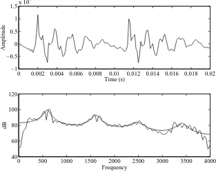
Figure 8: Representative frame of voiced speech (top) and its Fourier amplitude spectrum (bottom) with the smoothed spectrum of the LP analysis overlaid.
in pattern recognition and neural computation (Jacobs, Jordan, Nowlan, and Hinton 1991; Wolpert 1992) – although we must caution that the sub-band signals do not satisfy the (strong) assumption of independence (see above).
We consider first the wideband model. Figure 8 shows a typical frame of voiced speech from the word seven. The upper figure shows the 20 ms frame of speech and the lower diagram shows the Fourier am-plitude spectrum (in decibels) of the frame as well as the smoothed log-spectrum, generated from the im-pulse response of a filter created using the LP coefficients. The smoothed log-spectrum shows four peaks at approximately 600, 1600, 2500 and 3500 Hz.
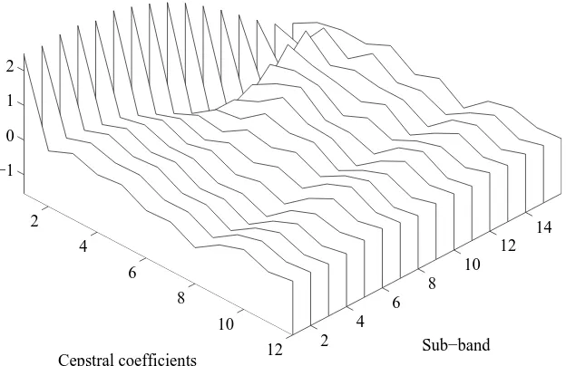
Figure 9 shows the smoothed log-spectra generated by the impulse responses of filters created using the LP coefficients. Here, the x -axis represents the frequency in hertz, the y-axis the sub-band index and the z-axis the spectral magnitude in decibels. The effects of the variations in LP coefficients across the 16 different models are readily visible in the spectrum. The poles of the filter (represented by the peaks in the smoothed spectrum) are clearly positioned at different frequencies in the different sub-bands. This is not surprising: after all, this emphasis of different frequencies is precisely what the filterbank is designed to do. In terms of data modeling, the poles of the LP filter are allocated to the particular areas of the spectrum which are prominent in each sub-band. Starting at the low-frequency end of the spectrum, the first sub-band has two prominent poles located below 800 Hz. As the index (center frequency) is increased, these two poles come closer together, until finally by sub-band 8 or 9 they are modeled as a single pole. As the index increases further, the influence of this low-frequency pole is reduced.
A similar effect is seen in the other frequency ranges as the filterbank emphasizes or de-emphasizes specific regions of the spectra. In particular, sub-bands 9–14 (center frequencies 1218–2659 Hz) locate many poles in the middle-frequency range which were absent from the low-frequency bands and also from the smoothed spectrum of the wideband analysis in Figure 8.
781
1563
2344
3125
3906 2
4 6
8 10
12 14 40
60 80
Frequency Sub−band
[image:16.612.141.463.90.309.2]dB
Figure 9: Smoothed sub-band LP spectra for the voiced frame of speech shown in Fig. 8.
2 4
6 8
10
12 2
4 6
8 10
12 14 −1
0 1 2
Cepstral coefficients Sub−band
[image:16.612.145.457.428.630.2]parameters of the LP model are constrained to be uniformly deployed across the selected frequency range, so that more parameters in total can be used without overfitting than with the wideband system where the modeling process does not feature this inbuilt constraint. Consequently, sub-band processing means that each speaker’s utterances are modeled in more detail than with a wideband approach. This improvement in modeling the speakers should lead in turn to improvements in speaker recognition performance, as observed here.
8
Conclusions and Discussion
Performance improvements through the use of sub-band processing have previously been reported for speech recognition, where the main motivation has been to introduce robustness against noise based on the presump-tion that narrow-band noise will affect some but not all channels. This paper has confirmed that performance improvements can be gained from sub-band processing in text-dependent speaker recognition, for clean speech. Other investigators have presented similar results but have not offered an explanation as to why sub-band pro-cessing actually works. Although the Fletcher-Allen principle – embodying general notions of how humans recognize speech – provides the background, it remains unclear precisely how performance benefits accrue. In this paper, we have advanced and explored the hypothesis that sub-band processing offers a practical solution to the bias/variance dilemma of data modeling. That is, unlike a wideband system, the free parameters of the speaker models are constrained to be more uniformly deployed across frequency so that more parameters in total can be used (so reducing bias) without incurring undue overfitting (variance) to spurious aspects of the speech signal – such as noise which is local in frequency or the roll-off of anti-alias filters. Hence, generaliza-tion to unseen data is improved.
The work here has used the sum rule of combination exclusively, in light of Kittler et al.’s (1998) finding that this is generally superior to alternatives, such as the product rule. However, weightings based on the speaker recognition performance of each individual sub-band gave no improvement on the unweighted sum. This is in keeping with Bourlard and Dupont’s (1996) findings, who found comparable error rates when they used the arithmetic mean and weightings similar to ours in sub-band speech recognition. Better results were only obtained through the non-linear MLP approach. However, they also found that, in narrow-band noise conditions, weightings based on phoneme recognition accuracy and on the signal-to-noise ratio of the sub-band gave lower error rates than did the arithmetic mean. Hence, although the results here have generally proved to be a significant improvement on wideband processing, there may be even greater gains to be had in noisy conditions. Accordingly, studies of sub-band speaker recognition with noisy speech are a priority for future work.
Our main conclusion is that sub-band processing can lead to improved speaker modeling by constraining the problem such that the free parameters of the model are fairly uniformly deployed across frequency. This improved modeling results in lower identification and verification error rates compared to the wideband ap-proach. However, much remains to be done to explore fully the new paradigm: the configuration used thus far may not be optimal. The 16 sub-bands were chosen a priori and spaced on the established psychophysical mel scale. We intend to study the effect on performance of using different numbers of filters, differently spaced in frequency. The LP model order (12th) for representing the outputs of the sub-band filters was chosen simply to be the same as for the wideband system (because the sampling rates are the same). It remains to be confirmed explicitly that the gains due to sub-band processing can not be achieved more cheaply by merely increasing the model order for the wideband system. Further work on the combination strategy is required to confirm that the sum rule does indeed outperform other rules of combination in this specific application. The num-ber of speakers in the database should also be varied and a wider range of speech materials studied to define better those circumstances in which sub-band processing is advantageous. The experimental system described here has been designed for simplicity so as to facilitate such exploration: it is not state-of-the-art. Yet it is a strong possibility that performance improvements by sub-band processing and subsequent information fusion are most easily (or only) obtained when the recognition methodology employed is itself only moderately capa-ble. Accordingly, another priority is to ascertain whether or not the same performance improvements could be obtained using sub-band processing in conjunction with state-of-the-art speaker recognition techniques such as Gaussian mixture models (Reynolds 1995).
science and technology. For instance, in audio-visual speech recognition, the issue of early versus late combi-nation is well known (e.g., Hennecke, Stork, and Venkatesh Prasad 1996). Early combicombi-nation fuses different sources of information into a single, large feature vector which forms the input to a single recognition sys-tem. Late combination uses different, independent recognition sub-systems whose outputs are fused. With the insights gained in this work, it is clear that early combination poses a large, relatively unconstrained data modeling problem and, consequently, late combination is much better advised.
References
Allen, J. B. (1994). How do humans process and recognize speech? IEEE Transactions on Speech and Audio Processing 2(4), 567–577.
Atal, B. S. (1974). Effectiveness of linear prediction characteristics of the speech wave for automatic speaker identification and verification. Journal of the Acoustical Society of America 55, 1304–1312.
Auckenthaler, R. and J. S. Mason (1997). Equalizing sub-band error rates in speaker recognition. In Eu-ropean Speech Communication Association (ESCA) Conference, Eurospeech 97, Rhodes, Greece, pp. 2303–2306.
Besacier, L. and J.-F. Bonastre (1997). Subband approach for automatic speaker recognition: optimal di-vision of the frequency domain. In Proceedings of 1st International Conference on Audio- and Visual-Based Biometric Person Authentication (AVBPA), Crans-Montana, Switzerland, pp. 195–202.
Bimbot, F. and L. Mathan (1994). Second-order statistical measures for text-independent speaker recogni-tion. In European Speech Communication Association (ESCA) Workshop on Automatic Speaker Recog-nition, Identification and Verification, Martigny, Switzerland, pp. 51–54.
Bishop, C. M. (1995). Neural Networks for Pattern Recognition. Oxford, UK: Clarendon Press.
Booth, I., M. Barlow, and B. Watson (1993). Enhancements to DTW and VQ decision algorithms for speaker recognition. Speech Communication 13, 427–433.
Bourlard, H. and S. Dupont (1996). A new ASR approach based on independent processing and recom-bination of partial frequency bands. In Proceedings of International Conference on Spoken Language Processing (ICSLP 96), Philadelphia, PA, pp. 426–429.
Bowles, R. L., R. I. Damper, and S. M. Lucas (1988). Combining evidence from separate speech recognition processes. In Proceedings of 7th FASE Symposium, Speech 88, Volume 2, Edinburgh, Scotland, pp. 669– 674.
Campbell, J. P. (1997). Speaker recognition: A tutorial. Proceedings of the IEEE 85(9), 1437–1462. Carey, M. J. and E. S. Parris (1992). Speaker verification using connected words. Proceedings of the Institute
of Acoustics 14(6), 95–100.
Cherkassky, V. and F. Mulier (1998). Learning from Data. New York, NY: John Wiley.
Damper, R. I. (1995). Introduction to Discrete-Time Signals and Systems. London: Chapman and Hall. Doddington, G. (1985). Speaker recognition – identifying people by their voices. Proceedings of the
IEEE 73(11), 1651–1664.
Doddington, G., W. Liggett, A. Martin, M. Przybocki, and D. Reynolds (1998). Sheep, goats, lambs and wolves: A statistical analysis of speaker performance in the NIST 1998 speaker recognition evaluation. In Proceedings of 5th International Conference on Spoken Language Processing, ICSLP 98, Sydney, Australia. Paper 608 on CD-ROM.
Finan, R. A. (1998). Towards the Use of Sub-Band Processing in Automatic Speaker Recognition. Ph. D. thesis, School of Engineering, University of Abertay Dundee.
Finan, R. A., A. T. Sapeluk, and R. I. Damper (1997). Impostor cohort selection for score normalisation in speaker verification. Pattern Recognition Letters 18, 881–888.
Gabor, D. (1946). Theory of communication. Journal of the Institution of Electrical Engineers 93, 429–457. Gabor, D. (1950). Communication theory and physics. Philosophical Magazine 4, 1161–1187.
Geman, S., E. Bienenstock, and R. Goursat (1992). Neural networks and the bias/variance dilemma. Neural Computation 4, 1–58.
Hennecke, M., D. G. Stork, and K. Venkatesh Prasad (1996). Visionary speech: looking ahead to practical speechreading systems. In D. G. Stork and M. Hennecke (Eds.), Speechreading by Humans and Ma-chines: Models, Systems and Applications, pp. 331–349. Berlin, Germany: NATO ASI Series, Springer.
Hermansky, H. (1998). Should recognizers have ears? Speech Communication 25(1–3), 3–27.
Hermansky, H. and N. Morgan (1994). RASTA processing of speech. IEEE Transactions on Speech and Audio Processing 2(4), 578–589.
Hermansky, H. and S. Sharma (1998). TRAPS – Classifiers of temporal patterns. In Proceedings of 5th International Conference on Spoken Language Processing, ICSLP 98, Sydney, Australia. Paper 615 on CD-ROM.
Hermansky, H., S. Tibrewala, and M. Pavel (1996). Towards ASR on partially corrupted speech. In Proceed-ings of 4th International Conference on Spoken Language Processing, ICSLP 96, Volume 1, Philadel-phia, PA, pp. 462–465.
Jacobs, R. A., M. I. Jordan, S. J. Nowlan, and G. E. Hinton (1991). Adaptive mixtures of local experts. Neural Computation 3, 79–87.
Kittler, J., M. Hatef, R. P. W. Duin, and J. Matas (1998). On combining classifiers. IEEE Transactions on Pattern Analysis and Machine Intelligence 20(3), 226–239.
Li, K.-P. and J. E. Porter (1988). Normalizations and selection of speech segments for speaker recognition scoring. In Proceedings of IEEE International Conference on Acoustics, Speech and Signal Processing, ICASSP 88, New York, NY, pp. 595–598.
Linde, J., A. Buzo, and R. M. Gray (1980). An algorithm for vector quantizer design. IEEE Transactions on Communications 28, 84–95.
Markel, J. D. and A. H. Gray (1976). Linear Prediction of Speech. Berlin, Germany: Springer-Verlag. Matsui, T. and S. Furui (1995). Likelihood normalization for speaker verification using phone- and
speaker-independent models. Speech Communication 17, 109–116.
Morris, A., A. Hagen, and H. Bourlard (1999). The full-combination sub-bands approach to noise robust HMM/ANN-based ASR. In Proceedings of 6th European Conference on Speech Communication and Technology (Eurospeech 99), Volume 2, Budapest, Hungary, pp. 599–602.
Naik, J. M., L. P. Netsch, and G. R. Doddington (1989). Speaker verification over long-distance tele-phone lines. In Proceedings of International Conference on Acoustics, Speech and Signal Processing, ICASSP 89, Volume 1, Glasgow, Scotland, pp. 524–527.
Okawa, S., E. Bocchieri, and A. Potamianos (1998). Multi-band speech recognition in noisy environments. In Proceedings of International Conference on Acoustics, Speech and Signal Processing, ICASSP 98, Volume I, Seattle, WA, pp. 641–641.
Owens, F. J. (1993). Signal Processing of Speech. Basingstoke, UK: Macmillan.
Picone, J. (1993). Signal modeling techniques in speech recognition. Proceedings of the IEEE 81, 1215– 1247.
Reynolds, D. A. (1994). Experimental evaluation of features for robust speaker identification. IEEE Trans-actions on Speech and Audio Processing 2(4), 639–643.
Reynolds, D. A. (1995). Speaker identification and verification using Gaussian mixture models. Speech Communication 17, 91–108.
Rosenberg, A. E. and S. Parthasarathy (1996). Speaker background models for connected digit password speaker verification. In Proceedings of IEEE International Conference on Acoustics, Speech and Signal Processing, ICASSP 96, Volume 1, Atlanta, GA, pp. 81–84.
Rosenberg, A. E. and F. K. Soong (1987). Evaluation of a vector quantization talker recognition system in text dependent and text independent modes. Computer Speech and Language 22, 143–157.
Schroeder, M. (1999). Computer Speech: Recognition, Compression and Synthesis. Berlin, Germany: Springer-Verlag.
Siegel, S. (1956). Nonparametric Statistics for the Behavioral Sciences. Tokyo, Japan: McGraw-Hill Ko-gakusha.
Sivakumaran, P., A. M. Ariyaeeinia, and J. A. Hewitt (1998). Sub-band speaker verification using dynamic recombination weights. In Proceedings of 5th International Conference on Spoken Language Processing, ICSLP 98, Sydney, Australia. Paper 1055 on CD-ROM.
Sivakumaran, P., A. M. Ariyaeeinia, J. A. Hewitt, and J. A. Malcolm (1998). An effective sub-band based approach for robust speaker verification. Proceedings of the Institute of Acoustics 20(6), 69–72. Steeneken, H. T. M. and T. Houtgast (1999). Mutual dependence of the octave-band weights in predicting
speech intelligibility. Speech Communication 28, 109–123.
Thompson, J. and J. S. Mason (1994). The pre-detection of error-prone class members at the enrollment stage of speaker recognition systems. In European Speech Communication Association (ESCA) Workshop on Automatic Speaker Recognition, Identification and Verification, Martigny, Switzerland, pp. 127–130.
Tibrewala, S. and H. Hermansky (1997). Sub-band based recognition of noisy speech. In Proceedings of International Conference on Acoustics, Speech and Signal Processing, ICASSP 97, Volume II, Munich, Germany, pp. 1255–1258.
Wolpert, D. H. (1992). Stacked generalization. Neural Networks 5, 241–259.
Yu, K., J. Mason, and J. Oglesby (1995). Speaker recognition using hidden Markov models, dynamic time warping and vector quantisation. IEE Proceedings: Vision, Image and Signal Processing 142, 313–318. Zwicker, E. and E. Terhardt (1980). Analytical expressions for critical-band rate and critical bandwidth as a