An Application of Newton Type Iterative Method
for Lavrentiev Regularization for Ill-Posed
Equations: Finite Dimensional Realization
Santhosh George and Suresan Pareth
Abstract—In this paper, we consider, a finite dimensional realization of Newton type iterative method for Lavrentiev regularization of ill-posed equations. Precisely we consider the ill-posed equation F(x) = f when the available data is fδ
with kf−fδk ≤δ and the operatorF :D(F)⊆X→X is a nonlinear monotone operator defined on a real Hilbert spaceX. The error estimate obtained under a general source condition onx0−xˆ(wherex0 is the initial guess andxˆis the solution of
F(x) = f) is of optimal order. The regularization parameter
α is chosen according to the adaptive method considered by Perverzev and Schock (2005). An example is provided to show the efficiency of the proposed method.
Index Terms—quartic convergence, Newton Lavrentiev method, monotone operator, ill-posed problems, adaptive method.
I. INTRODUCTION
An iteratively regularized projection method has been considered for apporoximately solving the ill-posed operator equation
F(x) =f (1)
where F : D(F) ⊆ X → X is a nonlinear monotone operator (i.e.,hF(x)−F(y), x−yi ≥0, ∀x, y∈D(F)) and
X is a real Hilbert space with the inner producth., .iand the normk.k.It is assumed that (1) has a solution, namelyˆxand
F possesses a locally uniformly bounded Fr´echet derivative
F′(x)for allx∈D(F)(cf. [14]) i.e.,
kF′(x)k ≤CF, x∈D(F) for some constant CF.
In application, usually only noisy data fδ are available, such that
kf−fδk ≤δ.
Then the problem of recovery of xˆ from noisy equation
F(x) =fδ is ill-posed, in the sense that a small perturbation
in the data can cause large deviation in the solution. For solving (1) with monotone operators (see [7], [12], [14], [15]) one usually use the Lavrentiev regularization method. In this method the regularized approximationxδ
α is obtained by solving the operator equation
F(x) +α(x−x0) =fδ. (2)
It is known (cf. [15], Theorem 1.1) that the equation (2) has a unique solution xδ
α forα >0, providedF is Fr´echet
differentiable and monotone in the ball Br(ˆx) ⊂ D(F)
Santhosh George and Suresan Pareth, Department of Mathemat-ical and Computational Sciences, National Institute of Technology Karnataka, Surathkal, India-575025, e-mail: [email protected], [email protected]
with radius r= kxˆ−x0k+δ/α. However the regularized equation (2) remains nonlinear and one may have difficulties in solving them numerically.
In [1], George and Elmahdy considered an iterative reg-ularization method which converges linearly to xδ
α and its finite dimensional realization in [2]. Later in [3] George and Elmahdy considered an iterative regularization method which converges quadratically to xδ
α and its finite dimensional realization in [4].
Recall that a sequence (xn) in X with limxn = x∗ is said to be convergent of orderp >1,if there exist positive reals β, γ,such that for alln∈N kxn−x∗k ≤βe−γp
n .If the sequence(xn)has the property that kxn−x∗k ≤βqn,
0 < q <1 then(xn)is said to be linearly convergent. For an extensive discussion of convergence rate (see [8]).
Note that the method considered in [1], [2], [3] and [4] are proved using a suitably constructed majorizing sequence which heavily depends on the initial guess and hence not suitable for practical consideration.
In an attempt to avoid majorizing sequence to prove the convergence of the method considered in [1], [2], [3] and [4], the authors considered in [5], a two step iterative method for solving (1), which converges linearly toxδ
α.Later in [11], the authors considered an application of Newton type iterative method, that converges quartically to xδ
α. In this paper we consider, finite dimensional realization of the method considered in [11].
The organization of this paper is as follows. Section 2 describes the method and its convergence. Section 3 deals with the error analysis and parameter choice strategy. Section 4 gives the algorithm for implementing the proposed method. Numerical example and computational results are given in section 5. Finally in section 6 we summarize the key points in the paper.
II. THEMETHOD AND ITSCONVERGENCE
Let{Ph}h>0be a family of orthogonal projections onX.
Our aim in this section is to obtain an approximation forxδ α, in the finite dimensional spaceR(Ph),the range ofPh.For the results that follow, we impose the following conditions.
Let
εh:=kF′(x)(I−Ph)k, ∀x∈D(F)
and{bh : h >0} is such thatlimh→0k(I−Pbhh)x0k = 0 and limh→0bh = 0. We assume that εh → 0 as h → 0. The above assumption is satisfied if, Ph → I pointwise and if
F′(x)is a compact operator. Further we assume thatε
h≤ε0,
bh≤b0 andδ∈(0, δ0].
IAENG International Journal of Applied Mathematics, 42:3, IJAM_42_3_07
A. Projection Method
We consider the following sequence defined iteratively by
yh,δ
n,α=xh,δn,α−R−α1(xh,δn,α)Ph[F(xh,δn,α)−fδ+α(xh,δn,α−x0)] (3) and
xh,δn+1,α =y h,δ
n,α−R−α1(yn,αh,δ)Ph[F(yh,δn,α)−fδ+α(yh,δn,α−x0)] (4) whereRα(x) :=PhF′(x)Ph+αPh andxh,δ0,α :=Phx0,for obtaining an approximation forxδ
α in the finite dimensional subspace R(Ph) of X. Note that the iteration (3) and (4) are the finite dimensional realization of the iteration (3) and (4) in [11]. We will be selecting the parameterα=αi from some finite set
DN ={αi: 0< α0< α1< α2<· · ·< αN}
using the adaptive method considered by Perverzev and Schock in [12].
We need the following assumptions for the convergence analysis.
Assumption 1: (cf. [14], Assumption 3) There exists a constant k0 ≥ 0 such that for every x, u ∈ D(F) and
v ∈ X there exists an element Φ(x, u, v) ∈ X such
that [F′(x)−F′(u)]v = F′(u)Φ(x, u, v),kΦ(x, u, v)k ≤
k0kvkkx−uk.
Assumption 2: There exists a continuous, strictly mono-tonically increasing function ϕ : (0, a] → (0,∞) with
a≥ kF′(ˆx)k satisfying;
(i) limλ→0ϕ(λ) = 0,
(ii) supλ≥0αϕλ+(αλ)≤cϕϕ(α) ∀λ∈(0, a]and
(iii) there existsv∈X withkvk ≤1(cf. [10]) such that
x0−xˆ=ϕ(F′(ˆx))v.
Let eh,δ
n,α := kyh,δn,α−xh,δn,αk, ∀n≥0 (5)
and for 0 < k0 < 2 3(1+ε0
α0)
, let g : (0,1) → (0,1) be the
function defined by
g(t) =27k
3 0
8 (1 +
ε0 α0)
3t3 ∀t∈(0,1). (6)
Hereafter we assume thatδ∈(0, δ0] whereδ0< α0.
Letb0<
q
1 + 2k0
(1+ε0 α0)
(1− δ0
α0)−1
k0 ,kxˆ−x0k ≤ρwhere
ρ <
q
1 + 2k0
(1+ε0 α0)
(1− δ0
α0)−1
k0 −b0 and
let γρ:= (1 +
ε0 α0)
k0
2 (ρ+b0)
2+ (ρ+b0)
+ δ0
α0. (7)
Lemma 1: Letx∈D(F). Then
kR−1
α (x)PhF′(x)k ≤(1 +
ε0 α0).
Proof. Note that,
kR−1
α (x)PhF′(x)k
= sup
kvk≤1
k(PhF′(x)Ph+αPh)−1PhF′(x)vk
= sup
kvk≤1
k(PhF′(x)Ph+αPh)−1PhF′(x)
(Ph+I−Ph)vk
≤ sup
kvk≤1
k(PhF′(x)Ph+αPh)−1PhF′(x)(Ph)vk+
sup
kvk≤1
k(PhF′(x)Ph+αPh)−1PhF′(x)(I−Ph)vk
≤ (1 +εh
α)
≤ (1 + ε0 α0).
Lemma 2: Lete0=eh,δ0,α andγρ be as in (7). Then
e0≤γρ.
Proof. Note that,
e0 = kyh,δ0,α−x h,δ
0,αk
= kR−α1(Phx0)Ph[F(Phx0)−fδ]k
= kR−α1(Phx0)Ph[F(Phx0)−F(ˆx)−F′(Phx0)
(Phx0−x) +ˆ F′(Phx0)(Phx0−x) +ˆ F(ˆx)−fδ]k
= kR−α1(Phx0)Ph
[
Z 1
0
(F′(ˆx+t(Phx0−x))ˆ −F′(Phx0))(Phx0−x)dtˆ
+F′(Phx0)(Phx0−x) +ˆ F(ˆx)−fδ]k
= kR−1
α (Phx0)PhF′(Phx0)
[
Z 1
0
Φ(ˆx+t(Phx0−x), Pˆ hx0, Phx0−x)dtˆ
+(Phx0−x)] +ˆ R−α1(Phx0)Ph(F(ˆx)−fδ)k and hence by Assumption 1, Lemma 1 and the relation
kR−1
α (Phx0)k ≤ α1,we have,
e0 ≤ (1 + ε0
α0)
k0
2 kPhx0−xˆk 2+kP
hx0−xˆk
+ δ
α
= (1 + ε0
α0)[ k0
2 kPhx0−x0+x0−xˆk
2
+kPhx0−x0+x0−xˆk] +
δ α
≤ (1 + ε0 α0)
k0
2 (ρ+bh)
2+ (ρ+b
h)
+ δ
α
≤ (1 + ε0 α0)
k0
2 (ρ+b0)
2+ (ρ+b0)
+ δ0
α0
= γρ. (8)
Lemma 3: Let yh,δ
n,α, xh,δn,α andeh,δn,α be as in (3), (4) and (5) respectively withδ∈(0, δ0].Then
(a) kxh,δ n,α−y
h,δ
n−1,αk ≤ 3k20(1 +
ε0
α0)(e
h,δ
n−1,α)2 and (b) kxh,δ
n,α−x h,δ
n−1,αk ≤[1 +3k20(1 +
ε0
α0)e
h,δ n−1,α]e
h,δ n−1,α. Proof. Observe that,
xh,δ
n,α−ynh,δ−1,α
= yh,δn−1,α−x h,δ n−1,α−R
−1
α (y h,δ n−1,α)Ph
[F(ynh,δ−1,α)−f
δ+α(yh,δ
n−1,α−x0)] +R
−1
α (x h,δ n−1,α)
Ph[F(xh,δn−1,α)−f
δ+α(xh,δ
n−1,α−x0)]
IAENG International Journal of Applied Mathematics, 42:3, IJAM_42_3_07
= ynh,δ−1,α−x h,δ
n−1,α−R−α1(y h,δ n−1,α)Ph
[F(yh,δn−1,α)−F(x h,δ
n−1,α) +α(y h,δ n−1,α−x
h,δ n−1,α)]
+[R−α1(x h,δ
n−1,α)−R−α1(y h,δ
n−1,α)]Ph[F(xh,δn−1,α)−fδ
+α(xh,δn−1,α−x0)]
= R−1
α (y h,δ
n−1,α)Ph[F′(yh,δn−1,α)(y h,δ n−1,α−x
h,δ n−1,α) −(F(ynh,δ−1,α)−F(xh,δn−1,α))] +R−α1(ynh,δ−1,α)Ph
(F′(yh,δ
n−1,α)−F′(x h,δ n−1,α))(x
h,δ n−1,α−y
h,δ n−1,α)
:= Γ1+ Γ2 (9)
where
Γ1 := R−α1(y
h,δ
n−1,α)Ph[F′(yh,δn−1,α)(y h,δ n−1,α−x
h,δ n−1,α) −(F(ynh,δ−1,α)−F(xh,δn−1,α))]
and
Γ2 := R−α1(yh,δn−1,α)Ph[F′(yh,δn−1,α)−F
′(xh,δ n−1,α)]
(xh,δn−1,α−yh,δn−1,α).
Note that,
kΓ1k
= kR−α1(y
h,δ n−1,α)Ph
Z 1
0
[F′(ynh,δ−1,α)−F′(x h,δ n−1,α
+t(yh,δn−1,α−x h,δ n−1,α))](y
h,δ n−1,α−x
h,δ n−1,α)dtk
= kR−α1(y
h,δ
n−1,α)PhF′(yh,δn−1,α) Z 1
0
[φ(xh,δn−1,α+
t(ynh,δ−1,α−x h,δ n−1,α), y
h,δ n−1,α, x
h,δ n−1,α−y
h,δ n−1,α)]dtk
≤ k0
2 (1 +
ε0 α0)ky
h,δ n−1,α−x
h,δ
n−1,αk2 (10) the last step follows from the Assumption 1 and Lemma 1. Similarly,
kΓ2k ≤ k0(1 + ε0
α0)ky
h,δ n−1,α−x
h,δ n−1,αk
2. (11)
So, (a) follows from (9), (10) and (11). And (b) follows from (a) and the triangle inequality;
kxh,δ n,α−x
h,δ
n−1,αk ≤ kxh,δn,α−y h,δ
n−1,αk+ky h,δ n−1,α−x
h,δ n−1,αk. THEOREM 1: Letyh,δ
n,α,xh,δn,αbe as in (3) and (4) respec-tively with δ∈(0, δ0] andeh,δ
n,α,g andγρ be as in equation (5), (6) and (7) respectively. Then
(a) kyh,δ
n,α−xh,δn,αk ≤g(e h,δ n−1,α)e
h,δ n−1,α; (b) g(eh,δ
n,α)≤g(γρ)4
n
, ∀n≥0;
(c) eh,δ
n,α≤g(γρ)
4n−1
3 γρ ∀n≥0.
Proof. We have,
yh,δ n,α−xh,δn,α
= xh,δ
n,α−y h,δ n−1,α−R
−1
α (xh,δn,α)Ph
[F(xh,δ
n,α)−fδ+α(xh,δn,α−x0)] +R−α1(yh,δn−1,α)
Ph[F(yh,δn−1,α)−fδ+α(y h,δ
n−1,α−x0)]
= xh,δ
n,α−yh,δn−1,α−R
−1
α (xh,δn,α)Ph
[F(xh,δn,α)−F(y h,δ
n−1,α) +α(x h,δ n,α−y
h,δ n−1,α)]
+[Rα−1(y h,δ
n−1,α)−R
−1
α (xh,δn,α)]Ph[F(ynh,δ−1,α)−f δ
+α(yh,δn−1,α−x0)]
= R−α1(xh,δn,α)Ph[F′(xh,δn,α)(xh,δn,α−y h,δ n−1,α) −(F(xh,δn,α)−F(y
h,δ
n−1,α))] +R−α1(xh,δn,α)Ph
[F′(xh,δn,α)−F′(y h,δ
n−1,α)]×(y h,δ
n−1,α−xh,δn,α)
:= Γ3+ Γ4 (12)
where
Γ3 := R−α1(xh,δn,α)Ph[F′(xh,δn,α)(xh,δn,α−y h,δ n−1,α) −(F(xh,δ
n,α)−F(y h,δ n−1,α))] and
Γ4 := R−α1(xh,δ
n,α)Ph[F′(xh,δn,α)−F
′(yh,δ n−1,α)]
(ynh,δ−1,α−xh,δ n,α).
Analogous to the proof of (10) and (11) one can prove that
kΓ3k ≤ k0
2 (1 +
ε0 α0)kx
h,δ n,α−y
h,δ
n−1,αk2 (13) and
kΓ4k ≤ k0(1 + ε0
α0)kx
h,δ
n,α−yh,δn−1,αk
2. (14)
Now (a) follows from the Lemma 3, (12), (13) and (14). Again, since for µ ∈ (0,1), g(µt) = µ3g(t), for all t ∈ (0,1),by (a) we get,
g(eh,δ
n,α)≤g(e0)
4n
(15)
and
eh,δn,α ≤ g(e
h,δ n−1,α)e
h,δ n−1,α ≤ g4n−1
(e0)g(eh,δn−2,α)e h,δ n−2,α ≤ g4n−1
(e0)g4n−2
(e0)g(eh,δn−3,α)e h,δ n−3,α ≤ g(e0)4n−1+4n−2+···+1
e0
≤ g(e0)4
n
−1
3 e0 (16)
providedeh,δ
n,α<1.Buteh,δn,α<1by Lemma 2, (6) and (16). Now (b) and (c) follow from (8), (15), (16) and the relation
g(e0)≤g(γρ).This completes the proof of the theorem.
THEOREM 2: Suppose0< g(γρ)<1 ,r= (1−g1(γρ)+
3k0 2 (1 +
ε0
α0)
γρ
1−g2(γρ))γρand let the assumptions of Theorem 1 hold. Thenxh,δ
n,α, yh,δn,α∈Br(Phx0)for alln≥0. Proof. Note that by (b) of Lemma 3 we have,
kxh,δ1,α−Phx0k = kxh,δ1,α−x h,δ
0,αk
≤ [1 +3k0
2 (1 +
ε0
α0)e0]e0 (17)
≤ [1 +3k0
2 (1 +
ε0 α0)γρ]γρ < r
i.e.,xh,δ1,α ∈Br(Phx0).Again note that from (17) and (a) of Theorem 1 we get,
kyh,δ1,α−Phx0k ≤ ky1h,δ,α−x h,δ
1,αk+kx h,δ
1,α−Phx0k
≤ g(e0)e0+ [1 +3k0
2 (1 +
ε0
α0)e0]e0
≤ [1 +g(e0) +3k0
2 (1 +
ε0
α0)e0]e0
≤ [1 +g(γρ) +
3k0
2 (1 +
ε0 α0)γρ]γρ < r
IAENG International Journal of Applied Mathematics, 42:3, IJAM_42_3_07
i.e.,yh,δ1,α∈Br(Phx0). Further by (17) and (b) of Lemma 3 we have,
kxh,δ2,α−Phx0k
≤ kxh,δ2,α−x h,δ
1,αk+kx h,δ
1,α−Phx0k
≤ [1 +3k0
2 (1 +
ε0
α0)e
h,δ
1,α]e h,δ
1,α+ [1 +
3k0
2 (1 +
ε0
α0)e0]e0
≤ [1 +3k0
2 (1 +
ε0
α0)g(e0)e0]g(e0)e0
+[1 +3k0
2 (1 +
ε0
α0)e0]e0
≤ [1 +g(e0) +3k0
2 (1 +
ε0
α0)e0(1 +g
2(e0))]e0 (18)
≤ [1 +g(γρ) +
3k0
2 (1 +
ε0
α0)γρ(1 +g 2(γ
ρ))]γρ
< r
and by (18) and (a) of Theorem 1 we have,
ky2h,δ,α−Phx0k
≤ ky2h,δ,α−x h,δ
2,αk+kx h,δ
2,α−Phx0k
≤ g(eh,δ1,α)e h,δ
1,α+ [1 +g(e0) +
3k0
2 (1 +
ε0
α0)e0
(1 +g2(e0))]e0
≤ g5(e0)e0+ [1 +g(e0) +3k0
2 (1 +
ε0
α0)e0
(1 +g2(e0))]e0
≤ [1 +g(e0) +g5(e0) +3k0
2 (1 +
ε0
α0)e0
(1 +g2(e0))]e0
≤ [1 +g(e0) +g2(e0) +3k0
2 (1 +
ε0
α0)e0
(1 +g2(e0))]e0
≤ [1 +g(γρ) +g2(γρ) +
3k0
2 (1 +
ε0 α0)γρ (1 +g2(γρ))]γρ
< r
i.e., xh,δ2,α, y h,δ
2,α ∈ Br(Phx0). Continuing this way one can prove thatxh,δ
n,α, yn,αh,δ ∈Br(Phx0),∀n≥0.This completes the proof.
The main result of this section is the following Theorem. THEOREM 3: Let 0 < g(γρ) <1, yn,αh,δ andxh,δn,α be as in (3) and (4) respectively withδ∈(0, δ0]and assumptions of the Theorem 2 hold. Then (xh,δ
n,α) is Cauchy sequence in Br(Phx0) and converges to xh,δα ∈ Br(Phx0). Further
Ph[F(xh,δα ) +α(xh,δα −x0)] =Phfδ and
kxh,δ
n,α−xh,δα k ≤Ce−γ4
n
whereC = ( 1 1−g(γρ)4 +
3k0γρ 2 (1 +
ε0
α0) 1
1−g2(γρ)4g(γρ) 4n
)γρ andγ=−logg(γρ).
Proof. Using the relation (b) of Lemma 3 and (c) of Theorem 1, we obtain,
kxh,δn+m,α−xh,δ n,αk
≤ m−1
X
i=0
kxh,δn+i+1,α−x h,δ n+i,αk
≤ m−1
X
i=0
1 +3k0e0
2 (1 +
ε0
α0)g(e0)
4n+i
g(e0)4n+ie0
≤ [(1 +g(e0)4+g(e0)42+· · ·+g(e0)4m)
+3k0e0
2 (1 +
ε0
α0)(1 +g
2(e0)4+g2(e0)42 +· · ·
+g2(e0)4m)g(e0)4n]g(e0)4ne0
≤ [(1 +g(γρ)4+g(γρ)4
2
+· · ·+g(γρ)4
m )
+3k0γρ
2 (1 +
ε0
α0)(1 +g
2(γ
ρ)4+g2(γρ)4
2 +· · ·
+g2(γρ)4
m )g(γρ)4
n ]g(γρ)4
n γρ ≤ Cg(γρ)4
n
≤ Ce−γ4n.
Thusxh,δ
n,α is a Cauchy sequence inBr(Phx0)and hence it converges, say toxh,δ
α ∈Br(Phx0). Observe that,
kPh[F(xh,δn,α)−fδ+α(xh,δn,α−x0)]k
= kRα(xh,δn,α)(xh,δn,α−yn,αh,δ)k ≤ kRα(xh,δn,α)kkxh,δn,α−yh,δn,αk
= k(PhF′(xh,δn,α)Ph+αPh)keh,δn,α
≤ (CF +α)g(γρ)4
n
γρ. (19)
Now by lettingn→ ∞ in (19) we obtain
Ph[F(xh,δα ) +α(xαh,δ−x0)] =Phfδ. (20)
This completes the proof.
III. ERRORBOUNDSUNDERSOURCECONDITIONS
The objective of this section is to obtain an error estimate forkxh,δ
n,α−xˆkunder a source condition on x0−x.ˆ
Proposition 1: LetF :D(F)⊆X →X be a monotone operator in X. Let xh,δ
α be the solution of (20) andxhα :=
xh,0
α . Then
kxh,δα −xhαk ≤
δ α.
Proof. The result follows from the monotonicity of F and the relation;
Ph[F(xh,δα )−F(xhα) +α(xαh,δ−xhα)] = Ph(fδ−f).
THEOREM 4: Let ρ < 2
k0(1+ ε0 α0)
and xˆ ∈ D(F) be a
solution of (1). And let Assumption 1, Assumption 2 and the assumptions in Proposition 1 be satisfied. Then
kxh
α−xˆk ≤C(ϕ(α) +˜
εh
α)
whereC˜:= max{1,ρ+kxˆk} 1−(1+ε0
α0) k0
2ρ .
Proof. Let M := R1
0 F
′(ˆx+t(xh
α−x))dt.ˆ Then from the
relation
Ph[F(xhα)−F(ˆx) +α(xhα−x0)] = 0
we have,
(PhM Ph+αPh)(xhα−ˆx) =Phα(x0−x) +ˆ PhM(I−Ph)ˆx.
IAENG International Journal of Applied Mathematics, 42:3, IJAM_42_3_07
Hence,
xh α−xˆ
= [(PhM Ph+αPh)−1Ph−(F′(ˆx) +αI)−1]α(x0−x)ˆ
+(F′(ˆx) +αI)−1α(x0−x)ˆ
+(PhM Ph+αPh)−1PhM(I−Ph)ˆx
= (PhM Ph+αPh)−1Ph[F′(ˆx)−M +M(I−Ph)]
(F′(ˆx) +αI)−1α(x0−x)ˆ
+(F′(ˆx) +αI)−1α(x0−x)ˆ
+(PhM Ph+αPh)−1PhM(I−Ph)ˆx
:= ζ1+ζ2 (21)
where
ζ1 := (PhM Ph+αPh)−1Ph[F′(ˆx)−M+M(I−Ph)]
(F′(ˆx) +αI)−1α(x0−x)ˆ
and
ζ2 := (F′(ˆx) +αI)−1α(x0−x) + (Pˆ
hM Ph+αPh)−1
PhM(I−Ph)ˆx.
Observe that,
kζ1k
≤ k(PhM Ph+αPh)−1Ph Z 1
0
[F′(ˆx)−F′(ˆx +t(xhα−x))]dt(Fˆ ′(ˆx) +αI)−1α(x0−x)ˆ k
+k(PhM Ph+αPh)−1PhM(I−Ph)
(F′(ˆx) +αI)−1α(x0−x)ˆ k
≤ k(PhM Ph+αPh)−1Ph Z 1
0
[F′(ˆx+t(xh
α−x))(Pˆ h+I−Ph)
φ(ˆx,xˆ+t(xhα−x),ˆ (F′(ˆx) +αI)−1α(x0−x))]dtˆ k
+εh
αρ
≤ (1 +εh
α)
k0
2 ρkx
h
α−xˆk+
εh
αρ
≤ (1 + ε0 α0)
k0
2ρkx
h
α−xˆk+
εh
αρ (22)
and
kζ2k ≤φ(α) +εh
αkxˆk. (23)
The result now follows from (21), (22) and (23). THEOREM 5: Letxh,δ
n,αbe as in (4). And the assumptions in Theorem 3 and Theorem 4 hold. Then
kxh,δ
n,α−xˆk ≤Ce
−γ4n
+max{1,C˜}(ϕ(α) +δ+εh
α ).
Proof., Observe that,
kxh,δn,α−xˆk ≤ kxh,δn,α−xh,δα k+kxh,δα −xhαk+kxhα−xˆk
so, by Proposition 1, Theorem 3 and Theorem 4 we obtain,
kxh,δ
n,α−xˆk ≤ Ce
−γ4n
+ δ
α+ ˜C(ϕ(α) +
εh
α)
≤ Ce−γ4n+max{1,C˜}(ϕ(α) +δ+εh
α ).
Let
nδ :=min
n:e−γ4n≤δ+εh
α
(24)
and
C0=C+max{1,C˜}. (25)
THEOREM 6: Let nδ and C0 be as in (24) and (25) respectively. And letxh,δ
nδ,αbe as in (4) and the assumptions
in Theorem 5 be satisfied. Then
kxh,δ
nδ,α−xˆk ≤C0(ϕ(α) + δ+εh
α ). (26)
A. A priori choice of the parameter
Note that the error estimate ϕ(α) + δ+εh
α in (26) is of optimal order ifαδ :=α(δ, h)satisfies,ϕ(αδ)αδ =δ+εh.
Now using the function ψ(λ) := λϕ−1(λ),0 < λ ≤ a
we have δ+εh = αδϕ(αδ) = ψ(ϕ(αδ)), so that αδ =
ϕ−1(ψ−1(δ+ε
h)). In view of the above observations and (26) we have the following.
THEOREM 7: Letψ(λ) :=λϕ−1(λ) for0< λ≤a, and
the assumptions in Theorem 6 hold. For δ > 0, let αδ =
ϕ−1(ψ−1(δ+ε
h))and letnδ be as in (24). Then
kxh,δ
nδ,α−xˆk=O(ψ
−1(δ+ε
h)).
B. An adaptive choice of the parameter
In this subsection, we present a parameter choice rule based on the balancing principle studied in [9], [12]. In this method, the regularization parameterαis selected from some finite set
DN(α) :={αi=µiα0, i= 0,1,· · ·, N}
whereµ >1, α0>0 and let
ni:=min
n:e−γ4n
≤δ+εh
αi
.
Then fori= 0,1,· · ·, N,we have
kxh,δni,αi−x
h,δ αik ≤C
δ+εh
αi
, ∀i= 0,1,· · ·N.
Letxi:=xh,δni,αi.In this paper we selectα=αifromDN(α)
for computingxi,for each i= 0,1,· · ·, N.
THEOREM 8: (cf. [14], Theorem 3.1) Assume that there existsi∈ {0,1,2,· · ·, N} such that ϕ(αi)≤ δ+αεih. Let the assumptions of Theorem 6 and Theorem 7 hold and let
l:=max
i:ϕ(αi)≤
δ+εh
αi
< N,
k:=max{i:kxi−xjk ≤4C0
δ+εh
αj
, j= 0,1,2,· · ·, i}.
Thenl≤kandkˆx−xkk ≤cψ−1(δ+εh)wherec= 6C0µ. IV. IMPLEMENTATION OF ADAPTIVE CHOICE RULE
Finally the balancing algorithm associated with the choice of the parameter specified in Theorem 1 involves the follow-ing steps:
• Chooseα0>0 such thatδ0< α0 andµ >1.
• Chooseαi :=µiα0, i= 0,1,2,· · ·, N.
IAENG International Journal of Applied Mathematics, 42:3, IJAM_42_3_07
A. Algorithm
1. Set i= 0.
2. Chooseni:=min n
n:e−γ4n
≤δ+εh
αi
o
.
3. Solvexi:=xh,δni,αi by using the iteration (3) and (4).
4. If kxi−xjk > 4C0δ+αεjh, j < i, then take k = i−1 and returnxk.
5. Else seti=i+ 1and go to 2.
V. NUMERICALEXAMPLE
In this section we consider the example considered in [14] for illustrating the algorithm considered in section IV. We apply the algorithm by choosing a sequence of finite dimen-sional subspace (Vn)ofX withdimVn =n+ 1.Precisely we chooseVn as the linear span of{v1, v2,· · ·, vn+1}where vi, i= 1,2,· · ·, n+ 1are the linear splines in a uniform grid of n+ 1 points in [0,1]. Note that xh,δ
n,α, yh,δn,α ∈ Vn. So
yh,δ n,α=
Pn+1
i=1 ξnivi andxh,δn,α= Pn+1
i=1 ηinvi, where ξin and
ηn
i, i= 1,2,· · ·, n+ 1are some scalars. Then from (3) we have
(PhF′(xh,δn,α) +α)(yh,δn,α−xh,δn,α) =Ph[fδ−F(xh,δn,α)
+α(xh,δ0,α−x h,δ
n,α)]. (27)
Observe that(yh,δ
n,α−xh,δn,α)is a solution of (27) if and only
if(ξn−ηn) = (ξn
1−ηn1, ξn2−η2n,· · ·, ξnn+1−ηnn+1)T is the
unique solution of
(Qn+αBn)(ξn−ηn) =Bn[ ¯µn−Fh1+α(X0−η¯n)](28)
where
Qn = [hF′(xh,δn,α)vi, vji], i, j= 1,2· · ·, n+ 1
Bn = [hvi, vji], i, j= 1,2· · ·, n+ 1
¯
µn = [fδ(t1), fδ(t2),· · ·, fδ(t
n+1)]T
Fh1 = [F(xh,δn,α)(t1), F(xn,αh,δ)(t2),· · ·, F(xh,δn,α)(tn+1)]T
X0 = [x0(t1), x0(t2),· · ·, x0(tn+1)]T
and t1, t2,· · ·, tn+1 are the grid points. Further from (4) it
follows that
(PhF′(yn,αh,δ) +α)(xh,δn+1,α−yh,δn,α) =Ph[fδ−F(yn,αh,δ)
+α(xh,δ0,α−yh,δn,α)] (29)
and hence(xh,δn+1,α−yn,αh,δ)is a solution of (29) if and only if
(ηn+1−ξn) = (ηn+1
1 −ξ1n, η2n+1−ξ2n,· · ·, ηnn+1+1−ξnn+1)T
is the unique solution of
(Tn+αBn)(ηn+1−ξn) =Bn[ ¯µn−Fh2+α(X0−ξ¯n)] (30)
where
Tn = [hF′(yh,δn,α)vi, vji], i, j= 1,2· · ·, n+ 1
Fh2 = [F(yh,δn,α)(t1), F(yn,αh,δ)(t2),· · ·, F(yn,αh,δ)(tn+1)]T.
Note that (28) and (30) are uniquely solvable asQn andTn are positive definite matrix (i.e.,xQnxT >0andxTnxT >0 for all non-zero vectorx) andBn is an invertible matrix.
EXAMPLE 4: (see [14], section 4.3) Let F : D(F) ⊆
L2(0,1)−→L2(0,1)defined by
F(u) :=
Z 1
0
k(t, s)u3(s)ds,
where
k(t, s) =
(1−t)s, 0≤s≤t≤1
(1−s)t, 0≤t≤s≤1 .
Then for all x(t), y(t) :x(t)> y(t) :
hF(x)−F(y), x−yi=
Z 1
0
Z 1
0
k(t, s)(x3−y3)(s)ds
×(x−y)(t)dt≥0.
Thus the operatorF is monotone. The Fr´echet derivative of
F is given by
F′(u)w= 3
Z 1
0
k(t, s)u2(s)w(s)ds. (31)
Note that foru, v >0,
[F′(v)−F′(u)]w= 3
Z 1
0
k(t, s)u2(s)ds
× R1
0 k(t, s)[v
2(s)−u2(s)]w(s)ds
R1
0 k(t, s)u2(s)ds
:=F′(u)Φ(v, u, w)
whereΦ(v, u, w) =
R1 0 k(t,s)[v
2(
s)−u2(
s)]w(s)ds R1
0 k(t,s)(u(s))
2ds .
Observe that
Φ(v, u, w) =
R1
0 k(t, s)[v2(s)−u2(s)]w(s)ds
R1
0 k(t, s)u2(s)ds
=
R1
0 k(t, s)[u(s) +v(s)][v(s)−u(s)]w(s)ds
R1
0 k(t, s)u2(s)ds
.
So Assumption 2 satisfies withk0≥
R1
0 k(t,s)[u(s)+v(s)]ds
R1 0k(t,s)u
2(s)ds
.
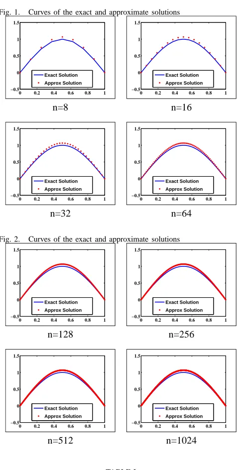
In our computation, we take f(t) = 6sin(πt9)+π2sin3(πt) and fδ=f+δ.Then the exact solution
ˆ
x(t) =sin(πt).
We use
x0(t) =sin(πt) +3[tπ
2−t2π2+sin2(πt)]
4π2
as our initial guess, so that the functionx0−xˆ satisfies the source condition
x0−xˆ=ϕ(F′(ˆx))1 4
whereϕ(λ) =λ.
For the operatorF′(.)defined in (31),ε
h=O(n−2)(cf. [6]). Thus we expect to obtain the rate of convergenceO((δ+ εh)
1 2).
We chooseα0= (1.1)(δ+εh), µ= 1.1, ρ= 0.11, γρ =
0.7818andg(γρ) = 0.99.The results of the computation are
presented in Table 1. The plots of the exact solution and the approximate solution obtained are given in Figures 1 and 2.
IAENG International Journal of Applied Mathematics, 42:3, IJAM_42_3_07
Fig. 1. Curves of the exact and approximate solutions
0 0.2 0.4 0.6 0.8 1 −0.5
0 0.5 1 1.5
Exact Solution Approx Solution
n=8
0 0.2 0.4 0.6 0.8 1 −0.5
0 0.5 1 1.5
Exact Solution Approx Solution
n=16
0 0.2 0.4 0.6 0.8 1 −0.5
0 0.5 1 1.5
Exact Solution Approx Solution
n=32
0 0.2 0.4 0.6 0.8 1 −0.5
0 0.5 1 1.5
Exact Solution Approx Solution
n=64
Fig. 2. Curves of the exact and approximate solutions
0 0.2 0.4 0.6 0.8 1 −0.5
0 0.5 1 1.5
Exact Solution Approx Solution
n=128
0 0.2 0.4 0.6 0.8 1 −0.5
0 0.5 1 1.5
Exact Solution Approx Solution
n=256
0 0.2 0.4 0.6 0.8 1 −0.5
0 0.5 1 1.5
Exact Solution Approx Solution
n=512
0 0.2 0.4 0.6 0.8 1 −0.5
0 0.5 1 1.5
Exact Solution Approx Solution
n=1024
TABLE I
ITERATIONS AND CORRESPONDING ERROR ESTIMATES
n k nk δ+εh α kxk−xˆk kxk−xˆk
(δ+εh)1/2 8 2 4 0.0135 0.0180 0.0356 0.3065 16 2 4 0.0134 0.0178 0.0432 0.3736 32 2 4 0.0133 0.0178 0.0450 0.3897 64 2 4 0.0133 0.0177 0.0455 0.3938
128 2 4 0.0133 0.0177 0.0456 0.3948 256 2 4 0.0133 0.0177 0.0456 0.3950 512 19 5 0.0133 0.0897 0.0456 0.3951 1024 27 6 0.0133 0.1923 0.0456 0.3951
VI. CONCLUSION
We have suggested and analyzed the finite dimensional realization of the iterative method considered in [11] for obtaining an approximate solution for nonlinear ill-posed operator equationF(x) =f when the operatorF :D(F)⊆
X →X defined on a real Hilbert spaceX is monotone, and the available data isfδ withkf−fδk ≤δ.Using a general source condition on x0−xˆ we obtained an optimal order
error estimate. The regularization parameter α is chosen according to the balancing principle considered by Perverzev and Schock (2005). The numerical results provided confirm the efficiency of the method.
ACKNOWLEDGMENT
S.Pareth thanks National Institute of Technology, Kar-nataka, India for the financial support.
REFERENCES
[1] S. George and A.I.Elmahdy, “An analysis of Lavrentiev regulariza-tion for nonlinear ill-posed problems using an iterative regularizaregulariza-tion method”, Int.J.Comput.Appl.Math., 2010, 5(3), pp. 369-381. [2] S. George and A.I.Elmahdy, ” An iteratively regularized projection
method for nonlinear ill-posed problems”, Int. J. Contemp. Math. Sciences, 2010, 5, no. 52, pp. 2547-2565.
[3] S. George and A.I.Elmahdy ”A quadratic convergence yielding iterative method for nonlinear ill-posed operator equations”, Comput. Methods Appl. Math, 2012, 12(1), pp. 3245
[4] S. George and A.I.Elmahdy, ” An iteratively regularized projection method with quadratic convergence for nonlinear ill-posed problems”, Int. J. of Math. Analysis, 2010, 4, no. 45, pp 2211-2228.
[5] S.George and S.Pareth, “Two-Step Modified Newton Method for Non-linear Lavrentiev Regularization”, ISRN Applied Mathematics, Volume 2012, Article ID 728627, 2012, doi:10.5402/2012/728627.
[6] C.W.Groetsch, J.T.King and D.Murio, “Asymptotic analysis of a finite element method for Fredholm equations of the first kind”, in Treatment of Integral Equations by Numerical Methods, Eds.: C.T.H.Baker and G.F.Miller, Academic Press, London, 1982, pp. 1-11.
[7] J.Jaan and U.Tautenhahn, “On Lavrentiev regularization for ill-posed problems in Hilbert scales”, Numer.Funct.Anal.Optim., 2003, 24, no. 5-6, pp. 531-555.
[8] C.T.Kelley, ”Iterative methods for linear and nonlinear equations”, SIAM Philadelphia, 1995.
[9] P.Mathe and S.V.Perverzev, “Geometry of linear ill-posed problems in variable Hilbert scales”, Inverse Problems, 2003, 19, no. 3, pp. 789-803. [10] M.T.Nair and P.Ravishankar, “Regularized versions of continuous Newton’s method and continuous modified Newton’s method under general source conditions”, Numer. Funct.Anal. Optim., 2008, 29(9-10), pp. 1140-1165.
[11] S.Pareth and S.George, “Newton type methods for Lavrentiev regular-ization of nonlinear ill-posed operator equations”, (2012), (communi-cated).
[12] S.V.Perverzev and E.Schock, “On the adaptive selection of the pa-rameter in regularization of ill-posed problems”, SIAM J.Numer.Anal., 2005, 43, pp. 2060-2076.
[13] A.G.Ramm, A.B.Smirnova and A.Favini, “Continuous modified Newton’s-type method for nonlinear operator equations” Ann.Mat.Pura Appl., 2003, 182, pp. 37-52.
[14] E.V.Semenova, “Lavrentiev regularization and balancing principle for solving ill-posed problems with monotone operators”, Comput. Methods Appl. Math., 2010, no.4, pp. 444-454.
[15] U.Tautanhahn, “On the method of Lavrentiev regularization for non-linear ill-posed problems”, Inverse Problems, 2002, 18 , pp. 191-207.
Santhosh George received his Ph.D in Mathematics from Goa University. He is currently working as an Associate Professor in the department of Mathematical and Computational Sciences, National Institute of Technology Karnataka, India. He has published several papers in international journals of good repute and proceedings of international conferences. His research interests include Functional Analysis, Inverse and Ill-posed problems and its applications. He has supervised many M.Tech dissertation. Two students have completed their Ph.D under his guidance. Currently three students are doing Ph.D under his guidance.
Suresan Pareth did MSc degree in Mathematics from the department of Mathematics Calicut University, Kerala, India. Also did MCA and M.Tech in Systems Analysis and Computer Applications from National Institute of Technology, Karnataka, India. His areas of interests are Analysis of algorithms, Inverse and Ill-posed problems and its applications. He worked as Assistant Director, Senior Software Developer, Assistant Professor and Associate Professor in Computer Science and Engineering. Currently he is a research scholar in the department of Mathematical and Computational Sciences, National Institute of Technology, Karnataka, India.