Generalized Diagonal Pivoting Methods
for Tridiagonal Systems without Interchanges
Jennifer B. Erway, Roummel F. Marcia, and Joseph A. Tyson
Abstract—It has been shown that a nonsingular symmetric tridiagonal linear system of the form T x = b can be solved in a backward-stable manner using diagonal pivoting meth-ods, where the LBLT decomposition of T is computed, i.e.,
T =LBLT, whereL is unit lower triangular andB is block diagonal with1×1and2×2blocks. In this paper, we generalize these methods for solving unsymmetric tridiagonal matrices. We present three algorithms that compute the LBMTfactorization, whereLandM are unit lower triangular andBis block diago-nal with1×1and2×2blocks. These algorithms are normwise backward stable and reduce to the LBLTfactorization when
applied to symmetric matrices. We demonstrate the robustness of the algorithms for the unsymmetric case using a wide range of well-conditioned and ill-conditioned linear systems. Numerical results suggest that these algorithms are comparable to Gaussian elimination with partial pivoting (GEPP). However, unlike GEPP, these algorithms do not require row interchanges, and thus, may be used in applications where row interchanges are not possible. In addition, substantial computational savings can be achieved by carefully managing the nonzero elements of the factorsL, B, andM.
Index Terms—linear algebra, tridiagonal systems, diagonal pivoting, Gaussian elimination.
I. INTRODUCTION
A
NONSINGULAR tridiagonal linear system of the formT x=b, (1)
whereT ∈IRn×n andxandb∈IRn, is often solved using
matrix factorizations. IfT is symmetric and positive definite, then the Cholesky decomposition or the LDLTfactorization, where L is a lower triangular matrix and D is a diagonal matrix, can be used to solve (1). If T is symmetric but indefinite, then diagonal pivoting methods can be used to form the LBLT factorization, where B is block diagonal with either 1×1 or 2×2 blocks, with row and/or column permutations (e.g., [1], [2], [3], [4]) or without (e.g., [2], [5], [6], [7]). Finally, ifT is unsymmetric, then (1) can be solved using Gaussian elimination with full pivoting or with partial pivoting (GEPP).
Based on previous works by the authors [8], [9], this paper generalizes diagonal pivoting methods for forming a backward-stable LBMT decomposition of a nonsingular tridiagonal matrix T without interchanges, where B is a
Manuscript received September 28, 2010. This work was supported by National Science Foundation grants DMS-0811106 and DMS-0811062. Portions of this work were presented at the World Congress of Engineers International Conference on Applied and Engineering Mathematics, London, UK, June/July 2010 and were published in the conference proceedings [9]. J.B. Erway is with the Department of Mathematics, Wake Forest University, Winston-Salem, NC, 27109 USA e-mail: (see http://www.wfu.edu/ ˜erwayjb/contact.html).
R.F. Marcia is with the School of Natural Sciences, Univer-sity of California, Merced, Merced, CA, 95343 USA e-mail: (see http://faculty.ucmerced.edu/rmarcia/contact.html).
J.A. Tyson is with the Department of Mathematics, Wake Forest Univer-sity, Winston-Salem, NC, 27109 USA
block diagonal matrix with either1×1 or2×2 blocks and Land M are unit-lower tridiagonal matrices. In this paper, we present three algorithms, two of which do not require the full matrix to be known a priori to form the factorization. We demonstrate that the resulting L, B, and M factors from the algorithm can be used to solve the linear system T x=b with accuracy comparable to Gaussian eliminiation with partial pivoting (GEPP). However, unlike GEPP, the algorithms we present do not use row interchanges, making them particularly useful in look-ahead Lanczos methods [10] and composite-step bi-conjugate gradient methods [11] for solving unsymmetric linear systems.
II. DIAGONAL PIVOTING
Let T ∈ IRn×n denote the unsymmetric nonsingular
tridiagonal matrix
T =
α1 γ2 0 · · · 0
β2 α2 γ3 . .. ...
0 β3 α3 . .. 0 ..
. . .. . .. . .. γn
0 · · · 0 βn αn
. (2)
We partitionT in the following manner:
T =
d n−d
d
n−d
B1 T12T T21 T22
(3)
The computation of the LBMTfactorization, whereLand M are unit lower triangular and B is block diagonal with
1×1 and 2×2 blocks, involves choosing the dimension (d= 1or 2) of the pivot B1 at each stage:
T =
Id 0
T21B1−1 In−d
B1 0
0 Sd
Id B1−1T12T
0 In−d
, (4)
whereSd =T22−T21B1−1T12T ∈IR(n−d)×(n−d). It can be shown that an invertible B1 exists for some dand that the Schur complementSd is tridiagonal so that the factorization
can be defined recursively. Specifically, ford= 1,
S1=T22−β2γ2 α1 e
(n−1)
1 e
(n−1)T
1 , (5)
wheree(1n−1) is the first column of the (n−1)×(n−1) identity matrix. Ford= 2,
S2=T22−
α1β3γ3 ∆
e(1n−2)e (n−2)T
1 .
where
∆=α1α2−β2γ2
is the determinant of the 2×2 pivot B1 and e(1n−2) is the first column of the(n−2)×(n−2)identity matrix. In both
IAENG International Journal of Applied Mathematics, 40:4, IJAM_40_4_07
cases Sd and T22 differ only in the (1,1) entry. Thus, the LBMTfactorization can be recursively defined to obtain the matricesL,B, andM, all the pivoting methods in this paper can be completely described by looking at the first stage of the factorization.
III. SYMMETRIC TRIDIAGONAL PIVOTING
Diagonal pivoting methods have its origins in the seminal works of Bunch [5], Bunch and Parlett [1], and Bunch and Kaufman [2] and have since been extended and expanded (see e.g., [3], [12], [13]). The factorization methods in these works generally solve dense symmetric indefinite systems using row and column interchanges. However, for symmetric tridiagonal matrices, diagonal pivoting methods have been developed that do not require row or column interchanges. In this section, we review these diagonal pivoting methods. Specifically, we let γj = βj for j = 2,3,· · ·, n in (2),
and consider the following nonsingular symmetric tridiagonal matrix:
T =
α1 β2 0 · · · 0
β2 α2 β3 . .. ...
0 β3 α3 . .. 0 ..
. . .. . .. . .. βn 0 · · · 0 βn αn
. (6)
The tridiagonal T can be partitioned similar to as before (see (3)). However, in the symmetric case, B1 andT22 are symmetric andT12=T21.
A. Bunch pivoting strategy
The diagonal pivoting method of Bunch [5] uses a1×1
pivot (i.e., d= 1) if the diagonal pivot is sufficiently large relative to the sub-diagonal entry. More precisely, if
σ= max
i,j |Ti,j|, (7)
a1×1 pivot is used in the first step if
σ|α1| ≥κβ22.
The choice ofκ, which is a root of the equationκ2+κ−1 =
0, balances the element growth in the Schur complement for both pivot sizes by equating the maximal element growth. Here
κ=
√ 5−1
2 ≈0.62. (8)
The Bunch pivoting strategy can be summarized as follows:
Algorithm B. This algorithm describes the first step in the pivoting strategy for symmetric tridiagonal matrices proposed in [5].
κ= (√5−1)/2≈0.62 σ= maxi,j|Ti,j| if σ|α1| ≥κβ22
dB= 1 else
dB= 2 end
A recursive application of Algorithm B yields a factoriza-tion T = LBLT, where L is unit lower triangular and B
is block diagonal. (In fact, one can show thatL andM are such thatLi,j= 0 for i−j >2.)
B. Bunch-Kaufman pivoting strategy
The pivoting strategy of Bunch requires that the largest element ofT be knowna priori. In some instances, we would like to be able to form the factorization asT is formed. The pivoting strategy of Bunch and Kaufman [2] circumvents this requirement by definingσ1, which is the largest element in magnitude “nearby” rather than the global maximum ofT in (7). More precisely, a1×1pivot is used in the first iteration if
σ1|α1| ≥κβ22,
where
σ1= max{|α2|,|β2|,|β3|}.
Note that this strategy is different from their well-known symmetric factorization using partial pivoting (see Sec. 4.2 of [2]). The Bunch-Kaufman pivoting strategy can be summarized as follows:
Algorithm BK. This algorithm is the tridiagonal pivoting strategy proposed in [2].
κ= (√5−1)/2≈0.62 σ1= max{|α2|,|β2|,|β3|}
if|α1|σ1≥κβ22, dBK = 1 else
dBK = 2 end
C. Bunch-Marcia pivoting strategy
Recently, Bunch and Marcia [6], [7] proposed diago-nal pivoting methods for symmetric indefinite tridiagodiago-nal matrices based on keeping the elements of the tridiagonal matrix L small, which is often an important property in many applications such as optimization. Here, we explicitly describe this pivoting strategy.
LetL1=T21B1−1in (4). If a1×1pivot is used, then the
(1,1)element ofL1 is
(L1)1,1= β2 α1
. (9)
If a2×2 pivot is used, then the (1,1)and(1,2) elements ofL1 are
(L1)1,1 = − β2β3
∆ , and (L1)1,2 = α1β3
∆ . (10) With the elements of L1 for a 2 ×2 pivot scaled by the constant κ (described above from the Bunch pivoting strategy [5]), Algorithm BM chooses a 1×1 pivot if the
(L1)1,1 in (9) is smaller than the largest entry in (10) in magnitude, i.e.,
|β2|
|α1|
≤ maxκ
|β
2β3|
|∆| , |α1β3|
|∆|
, (11)
and a 2 ×2 pivot is chosen otherwise. In other words, Algorithm BM chooses pivot sizes based on whichever leads
IAENG International Journal of Applied Mathematics, 40:4, IJAM_40_4_07
to smaller entries (in magintude) in the computed factor L. In [7], an additional criterion is imposed that if
|α1α2| ≥κβ22 (12)
a1×1pivot is chosen. This additional criterion guarantees that ifT is positive definite, the LBLTfactorization reduces to the LDLTfactorization. The choice of pivot size in the first iteration is described as follows:
Algorithm BM. This algorithm is the simplified tridiagonal pivoting strategy for symmetric tridiagonal matrices proposed in [7].
κ= (√5−1)/2≈0.62 ∆=α1α2−β22
if |α1α2| ≥κβ22 or |∆| ≤κ|α1β3| or |β2∆| ≤κ|α21β3| dBM = 1
else
dBM = 2 end
Intuitively, Algorithm BM chooses a 1 × 1 pivot if α1 is sufficiently large relative to the determinant of the
2×2 pivot, i.e., a 1×1 pivot is chosen if a2×2 pivot is relatively closer to being singular than α1 is to zero.
IV. UNSYMMETRIC CASE GENERALIZATION
In this section, we generalize the diagonal pivoting meth-ods for symmetric tridiagonal matrices described in Sec. III to unsymmetric systems. We now describe these methods, characterize relationships between the methods, and show the three methods are normwise backward stable.
A. Unsymmetric Bunch pivoting
The Bunch pivoting strategy can be extended to unsym-metric tridiagonal matrices by choosing a 1×1 pivot if
|α1|σ=κ|β2γ2|,
where σ is as before in (7), and a 2×2 pivot otherwise. (We prove the backward stability of this pivoting strategy in Sec. IV-F.)
Algorithm UB. This algorithm describes the first step of the unsymmetric Bunch pivoting strategy.
κ= (√5−1)/2≈0.62 σ= maxi,j|Ti,j| if σ|α1| ≥κ|β2γ2|
dU B = 1 else
dU B = 2 end
B. Unsymmetric Bunch-Kaufman pivoting
In [8], we generalized the pivoting strategy of Bunch and Kaufman for symmetric tridiagonal matrices (Algorithm BK). This pivoting strategy chooses a 1 ×1 pivot if the
(1,1) diagonal entry is sufficiently large relative to the off-diagonals, i.e.,
|α1|σ1≥κ|β2γ2|,
where
σ1= max{|α2|,|γ2|,|β2|,|γ3|,|β3|},
and κ is as in Sec. 2.1. This algorithm can be viewed as a generalization of the Bunch-Kaufman algorithm to the unsymmetric case.
Algorithm UBK. This alternative algorithm determines the size of the pivot for the first stage of the LBMT factorization applied to a tridiagonal matrixT ∈IRn×n.
κ= (√5−1)/2≈0.62
σ1= max{|α2|,|γ2|,|β2|,|γ3|,|β3|}
if|α1|σ1≥κ|β2γ2|, dII = 1
else
dII = 2 end
C. Unsymmetric Bunch-Marcia pivoting
The Bunch-Marcia pivoting strategy can be generalized to unsymmetric tridiagonal matrices by the following. Let
L1=T21B−11 and M
T
1 =B
−1 1 T
T
12
in (4). If a 1×1 pivot is used, then the(1,1) elements of L1 andM1 are
(L1)1,1= β2 α1
and (M1)1,1= γ2 α1
. (13)
If a2×2 pivot is used, then the (1,1)and(1,2) elements ofL1 andM1 are
(L1)1,1 = − β2β3
∆ , (M1)1,1 = − γ2γ3
∆ ,
(L1)1,2 = α1β3
∆ , (M1)1,2 =
α1γ3 ∆ .
(14)
With the elements ofL1 andM1 for a2×2 pivot scaled by the constantκas before in (8), the unsymmetric Bunch-Marcia pivoting strategy (Algorithm UBM) chooses a1×1
pivot if the both of the entries in (13) is smaller than the largest entry in (14) in magnitude, i.e.,
max|β2|
|α1| , |γ2|
|α1|
≤maxκ
|β2β3|
|∆| , |α1β3|
|∆| , |γ2γ3|
|∆| , |α1γ3|
|∆|
,
(15) and a 2 ×2 pivot is chosen otherwise. In other words, Algorithm UBM chooses pivot sizes based on whichever leads to smaller entries (in magintude) in the computed factorsL and M. In addition, we impose the criterion that if
|α1α2| ≥κ|β2γ2|, (16)
a1×1 pivot is chosen. This additional criterion guarantees that ifT is positive definite, the LBMTfactorization reduces to the LDMTfactorization. The choice of pivot size in the first iteration is described as follows:
Algorithm UBM. This algorithm determines the size of the pivot for the first stage of the LBMT factorization applied to a tridiagonal matrixT ∈IRn×n.
IAENG International Journal of Applied Mathematics, 40:4, IJAM_40_4_07
κ= (√5−1)/2≈0.62 ∆=α1α2−β2γ2
if |α1α2| ≥κ|β2γ2| or |∆|max{|β2|,|γ2|} ≤
κ|α1|max{|β2β3|,|α1β3|,|γ2γ3|,|α1γ3|} dU BM = 1
else
dU BM = 2 end
D. Relationships of the pivoting strategies
In this section, we summarize the relationship between the three pivoting strategies for unsymmetric matrices. In [8], it was shown that if the unsymmetric Bunch-Marcia pivoting strategy chooses a 1×1 pivot, i.e., dU BM = 1, then the
unsymmetric Bunch-Kaufman pivoting strategy also chooses a1×1pivot, i.e.,dU BK= 1. Conversely, ifdU BK= 2, then
dU BM = 2 as well. Finally, if dU BM = 2 and dU BK = 1,
then the subsequent unsymmetric Bunch-Kaufman pivot size will also be 1×1. This implies that the difference between Algorithm UBK and Algorithm UBM is that sometimes the unsymmetric Bunch-Marcia pivoting strategy chooses a
2×2pivot while the unsymmetric Bunch-Kaufman pivoting strategy chooses two 1×1 pivots. In this section, we relate the pivot sizes these two methods to the unsymmetric Bunch pivoting strategy.
Lemma 1. If dUBK = 1, then dUB = 1. If dUB = 2, thendUBK = 2. And, ifdUBK = 2anddUB = 1, then the subsequent unsymmetric Bunch pivot is1×1. In other words, the two pivoting strategies differ only when the unsymmetric Bunch-Kaufman strategy chooses a 2 ×2 pivot while the unsymmetric Bunch pivoting strategy chooses two 1 ×1 pivots.
Proof. SupposedUBK = 1. Sinceσ1≤σ, then
|α1|σ≥ |α1|σ1≥κ|β2γ2|,
which implies that dUB = 1. Similarly, if dUB = 2, then
dUBK= 2. Now, ifdUBK = 2, then the unsymmetric
Bunch-Marcia pivot size is dUBM = 2(as described above), which
implies that∆ > κ|α1||β3|in (15). Thus
|(S1)1,1|σ =
∆ α1
σ > κ|β3|γ3|,
where (S1)1,1 ≡ α2 −β2γ2/α1 = ∆/α1 is the (1,1) entry of the Schur complement S1 defined in (5). Thus, the subsequent unsymmetric Bunch pivot size is 1, which proves the lemma.
The following table relates the pivot sizes for the three algorithms:
TABLE I: At any given iteration step, this table summarizes all the possible pivot size choices for the three algorithms discussed in this section (Algorithms UB, UBK, and UBM).
UB UBK UBM
One1×1 One1×1 One1×1 Two1×1 Two1×1
One2×2 Two1×1 One2×2
One2×2
Finally, ifT is positive definite, then
|α1α2| ≥ |β2γ2| ≥κ|β2γ2|,
which implies that Algorithm UBM will always choose a
1×1pivot. Similarly, Algorithms UB and UBK will always choose a1×1 pivot because
|α1|σ≥ |α1|σ1≥ |α1α2|.
This leads to the following result:
Proposition 1. If T is a positive definite tridiagonal matrix, then the LBMTfactorization using Algorithms UB, UBK, or UBM reduces to the LDMTfactorization, whereL andM are unit lower triangular andDis diagonal.
E. Connections to the symmetric case
When applied to a symmetric tridiagional matrix, the three algorithms for unsymmetric tridiagonal matrices described in Sec. IV reduce to the symmetric methods described in Sec. III.
The following two lemmas show that Algorithm UB and UBK are unsymmetric generalizations of Algorithm B and BK, respectively. In other words, on symmetric matrices Algorithms UB and UBK reduce to Algorithms B and BK, respectively.
Lemma 2. Let T be a nonsingular symmetric matrix as in (6). Algorithm B chooses a 1 × 1 pivot if and only if Algorithm UB chooses a1×1pivot. Moreover, Algorithm B chooses a2×2pivot if and only if Algorithm UB chooses a 2×2pivot.
Proof.Whenβ2=γ2, Algorithms B and UB are identical.
Lemma 3. Let T be a nonsingular symmetric matrix as in (6). Algorithm BK chooses a1×1pivot if and only if the Algorithm UBK chooses a1×1pivot. Moreover, Algorithm BK chooses a 2 ×2 pivot if and only if Algorithm UBK chooses a2×2pivot.
Proof. Substituting β2 = γ2 and β3 = γ3 into Algorithm UBK gives the result.
The following lemma shows that Algorithm UBM is a generalization of Algorithm BM in the sense that on symmetric matrices, both algorithms choose the same pivots.
Lemma 4. Let T be a nonsingular symmetric matrix as in (6). Algorithm BM chooses a 1 × 1 pivot if and only if Algorithm UBM chooses a 1 ×1 pivot. Algorithm BM chooses a2×2pivot if and only if Algorithm UBM chooses a2×2pivot.
Proof. If Algorithm BM chooses a 1×1 pivot then either
|α1α2| ≥κβ22or|∆||β2| ≤κ|α1|max{|β2β3|,|α1β3|}. The latter condition is equivalent to either|∆β2| ≤κ|α1||β2β3| or |∆β2| ≤ κ|α21β3|. Thus, if Algorithm BM chooses a
1×1 pivot then
|α1α2| ≥κβ22 or |∆| ≤κ|α1β3| or|β2∆| ≤κ|α21β3|,
IAENG International Journal of Applied Mathematics, 40:4, IJAM_40_4_07
satisfying the conditions for which Algorithm UBM will also choose a 1 ×1 pivot. Reversing this argument shows that if Algorithm UBM chooses a 1×1 pivot then Algorithm BM will do the same. The second statement of the lemma follows since it is the contrapositive of the first.
The following proposition summarizes the lemmas in this section:
Proposition 2. If T is a symmetric tridiagonal matrix, then Algorithms UB, UBK, and UBM reduce to Algorithms B, BK, and BM, respectively. If T is also positive definite, then the LBMTfactorization reduces to the LDLT.
F. Backward stability result
In [8], we showed that Algorithms UBK and UBM imply a backward stability result that demonstrates that (a) the difference between computed factorization LbBbMcT and the
original tridiagonal matrix T is small (i.e., it is of order machine precision), and (b) the computed solution xb is the exact solution to a nearby problem. Using the relationship between the pivots of Algorithms UB and UBM and using arguments similar to that in [8], we can easily show the same results for Algorithm UB. More formally, we state the following theorem:
Theorem 1. Assume the LBMT factorization of the unsymmetric tridiagonal matrixT ∈ IRn×n obtained using the pivoting strategy of Algorithm UB, UBK, or UBM yields the computed factorization T ≈ LbBbMcT, and let xb be the
computed solution toT x=bobtained using the factorization. Assume that all linear systemsEy=f involving2×2pivots
Eare solved using the explicit inverse. Then
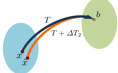
T−LbBbMcT =∆T1, and (T +∆T2)xb=b,
where
k∆Tikmax≤cukTkmax+O(u2), i= 1,2,
wherecis a constant anduis the machine precision.
Proof. See [8].
Pictorially, the backward stability result of Theorem 1 is represented in Fig. 1.
V. NUMERICAL EXPERIMENTS
Numerical tests were run using MATLABimplementations of Algorithm UB, UBK, UBM, GEPP, and the MATLAB
backslash command (“\”). (Specifically, Algorithms UB, UBK, and UBM were embedded in a code that used one forward substitution to solve with L, one back substitution to solve withMT, and a solve with the block-diagonal factor
B). We compared the performance of each code on 16 types of nonsingular tridiagonal linear systems of the formT x=b. The test set of system matrices contains a wide range of difficulty. Many ill-conditioned matrices were chosen as part of the test set in order to compare algorithm robustness. (Ill-conditioned matrices are often challenging for matrix-factorization algorithms.) The test set of system matrices was taken from recent literature (specifically, [14] and [15])
b
x
ˆ
x
T
[image:5.595.328.520.64.183.2]T
+
∆T
2Fig. 1: Theorem 1 implies not only that the product of the computed factorsLbBbMcT is very close to the original matrix
T, but that the computed solutionxˆ is the exact solution to a nearby problem, i.e., the components of the perturbation matrix∆T2 are very small.
on estimating condition numbers of ill-conditioned matrices– a task that can become increasingly difficult the more ill-conditioned the matrix is.
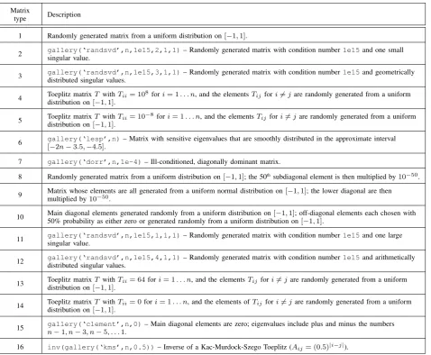
Table II contains a description of each tridiagonal matrix type in the test set. The first ten matrix types listed are based on test cases in [15]. Types 11-14 correspond to test cases found in [14] not found in [15], i.e., we eliminated redundant types. Finally, we include two additional tridiagonal matrices (Types 15-16) that can be generated using the MATLAB
command gallery. For our test, T was chosen to be a
100×100 matrix. The elements of b were chosen from a uniform distribution on[−1,1].
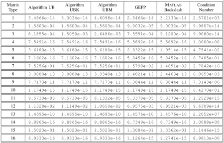
One system matrix was generated from each matrix type, and together with a vector b, the same linear system of the formT x=bwas solved by each algorithm. Table III shows the relative errors associated with each method. Columns 2-6 of the table contain the relative error
Erel =
kTxˆ−bk2
kbk2 ,
wherexˆ is the computed solution by each solver. The final column gives the condition number of the system matrixT. Each row in the table corresponds to one linear system from one type; that is, rowicontains the relative errors associated with each solver on a linear system whose system matrix was from typei in Table II. Although we only present one set of results in this paper, these results are representative of the many runs we performed.
Table III suggests that all five algorithms are comparable on a wide variety of linear systems. When the system matrix is well-conditioned (e.g., Types 1, 4, 5, 6, 8, 10, 14, 16), the algorithms have relative errors that are close to machine precision and that are comparable to one another. On the other hand, more significant differences occur when the system matrix is very ill-conditioned (Types 2, 3, 7, 11, 12 and 15). For example, on Type 13, Algorithms UB, UBK, and UBM perform particularly poorly, and the solutions are offered by GEPP and the MATLABbackslash command are also very poor, with an error near10−1. In fact, due to the ill-conditioning of the system matrix, all methods failed to solve the linear system; however, all methods obtain relative errors within an order of magnitude of each other. Meanwhile,
IAENG International Journal of Applied Mathematics, 40:4, IJAM_40_4_07
TABLE II: Tridiagonal matrix types used in the numerical experiments.
Matrix
type Description
1 Randomly generated matrix from a uniform distribution on[−1,1].
2 gallery(‘randsvd’,n,1e15,2,1,1)– Randomly generated matrix with condition number1e15and one small singular value.
3 gallery(‘randsvd’,n,1e15,3,1,1)– Randomly generated matrix with condition number1e15and geometrically distributed singular values.
4 Toeplitz matrixT withTii= 10
8 fori= 1. . . n, and the elementsT
ijfori6=jare randomly generated from a uniform
distribution on[−1,1].
5 Toeplitz matrixT withTii= 10
−8 fori= 1. . . n, and the elementsT
ijfori6=jare randomly generated from a uniform
distribution on[−1,1].
6 gallery(‘lesp’,n)– Matrix with sensitive eigenvalues that are smoothly distributed in the approximate interval [−2n−3.5,−4.5].
7 gallery(‘dorr’,n,1e-4)– Ill-conditioned, diagonally dominant matrix.
8 Randomly generated matrix from a uniform distribution on[−1,1]; the 50thsubdiagonal element is then multiplied by10−50. 9 Matrix whose elements are all generated from a uniform normal distribution on[−1,1]; the lower diagonal are then
multiplied by10−50.
10 Main diagonal elements generated randomly from a uniform distribution on[−1,1]; off-diagonal elements each chosen with 50% probability as either zero or generated randomly from a uniform distribution on[−1,1].
11 gallery(‘randsvd’,n,1e15,1,1,1)– Randomly generated matrix with condition number1e15and one large singular value.
12 gallery(‘randsvd’,n,1e15,4,1,1)distributed singular values. – Randomly generated matrix with condition number1e15and arithmetically
13 Toeplitz matrixdistribution on[T−1with,1].Tii= 64fori= 1. . . n, and the elementsTijfori6=jare randomly generated from a uniform
14 Toeplitz matrixdistribution on[T−1with,1].Tii= 0fori= 1. . . n, and the elements ofTijfori6=jare randomly generated from a uniform
15 gallery(‘clement’,n,0)– Main diagonal elements are zero; eigenvalues include plus and minus the numbers
n−1, n−3, n−5, . . .1.
16 inv(gallery(‘kms’,n,0.5))– Inverse of a Kac-Murdock-Szego Toeplitz (Aij= (0.5)|i−j|).
Types 9 and 13 have larger condition numbers and relative errors that slightly larger than machine precision; on these problems all algorithms have nearly identical relative errors (i.e., same order of magnitude).
VI. CONCLUSIONS AND FUTURE WORK
Algorithms UB, UBK, and UBM presented in this paper were shown to compute a backward-stable LBMT decomposi-tion of any nonsingular tridiagonal matrix without using row or column interchanges. In this paper, we showed that these algorithms can be viewed as generalizations of algorithms for symmetric tridiagonal matrices by comparing their choice of pivot sizes on symmetric tridiagonal matrices. Moreover, we established relationships between pivot choices made by each unsymmetric algorithms on general unsymmetric tridiagonal matrices. Numerical results presented in this paper on a wide range of linear systems suggest that the performance of these algorithms are comparable to GEPP and the MATLAB
backslash command.
In addition to computing a backward-stable LBMT de-composition of T, these algorithms have minimal storage requirements. Specifically, T is tridiagonal, and thus, can stored using three vectors. Moreover, updating the Schur complement requires updating only one nonzero component
of T. The matrices L andM are unit-lower triangular with Li,j = Mi,j = 0 for i−j > 2; thus, their entries can be
stored in two vectors each. Finally,Bis block-diagonal with
1×1or2×2blocks, requiring only three vectors for storage. Of the three strategies, Algorithms UBK and UBM do not depend on knowing the largest entry ofT a priori, making them suitable to factorize T as it is being formed. Thus, future work will focus on embedding Algorithms UBK and UBM into methods such as the look-ahead Lanczos methods [10] and composite-step bi-conjugate gradient methods [11] for solving unsymmetric linear systems.
REFERENCES
[1] J. R. BUNCH AND B. N. PARLETT, Direct methods for solving symmetric indefinite systems of linear equations, SIAM J. Numer. Anal., 8, pp. 639–655, 1971.
[2] J. R. BUNCH ANDL. KAUFMAN,Some stable methods for calculating inertia and solving symmetric linear systems, Math. Comp., 31, pp. 163–179, 1977.
[3] C. ASHCRAFT, R. G. GRIMES,ANDJ. G. LEWIS,Accurate symmetric indefinite linear equation solvers, SIAM J. Matrix Anal. Appl., 20, pp. 513–561, 1999.
[4] H. R. FANG ANDD. P. O’LEARY,Stable factorizations of symmetric tridiagonal and triadic matrices, SIAM J. Matrix Anal. Appl., 28, pp. 576–595, 2006.
[5] J. R. BUNCH, Partial pivoting strategies for symmetric matrices, SIAM J. Numer. Anal., 11, pp. 521–528, 1974.
IAENG International Journal of Applied Mathematics, 40:4, IJAM_40_4_07
TABLE III: Relative errors for five methods for solving the tridiagonal systemT x=b.
Matrix
Type Algorithm UB
Algorithm UBK
Algorithm
UBM GEPP
MATLAB
Backslash
Condition Number
1 3.4866e-14 3.3034e-14 4.6098e-14 2.5466e-14 3.2133e-14 2.5701e+03
2 1.5603e-04 1.5603e-04 1.5603e-04 9.0032e-05 9.0032e-05 9.9807e+14
3 8.1855e-04 1.5050e-03 2.6486e-03 7.5551e-04 9.1200e-04 9.9080e+14
4 7.5491e-16 7.5491e-16 7.5491e-16 5.5892e-16 5.5892e-16 1.0000e+00
5 3.6180e-15 3.6180e-15 3.6180e-15 2.8322e-15 1.9514e-15 4.7541e+02
6 7.1602e-16 7.1602e-16 7.1602e-16 5.8452e-16 5.8452e-16 6.7485e+01
7 7.5256e+01 7.5256e+01 7.5256e+01 1.5790e+02 1.4851e+02 2.7842e+16
8 3.0088e-13 3.0088e-13 3.9340e-13 2.4821e-13 2.4463e-13 6.9653e+03
9 7.7173e-11 7.7173e-11 7.7173e-11 6.3844e-11 6.3844e-11 7.3143e+06
10 1.1749e-15 1.1749e-15 1.1749e-15 1.1749e-15 1.1749e-15 6.4270e+01
11 9.5730e-05 9.5730e-05 8.1332e-05 5.3370e-05 5.3370e-05 1.2529e+15
12 1.1328e-02 1.1149e-02 1.0650e-02 6.9575e-03 6.9521e-03 9.6309e+14
13 1.4695e-10 1.4695e-10 1.4695e-10 1.4576e-10 1.4576e-10 2.2052e+07
14 9.8865e-16 9.8865e-16 9.8865e-16 6.7349e-16 6.7349e-16 1.0088e+00
15 1.5023e-01 1.5023e-01 1.5023e-01 1.3084e-01 1.3362e-01 3.1446e+15
16 6.9333e-16 6.9333e-16 6.9333e-16 1.1264e-15 1.2741e-15 8.9813e+00
[6] J. R. BUNCH ANDR. F. MARCIA,A pivoting strategy for symmetric tridiagonal matrices, Numer. Linear Algebra Appl., 12, pp. 911–922, 2005.
[7] J. R. BUNCH ANDR. F. MARCIA,A simplified pivoting strategy for symmetric tridiagonal matrices, Numer. Linear Algebra Appl., 13, pp. 865–867, 2006.
[8] J. B. ERWAY ANDR. F. MARCIA,A backward stability analysis of di-agonal pivoting methods for solving unsymmetric trididi-agonal systems without interchanges. Numerical Linear Algebra with Applications, n/a. doi: 10.10002/nla.674.
[9] J. B. ERWAY, R. F. MARCIA,ANDJ. TYSON,On solving unsymmetric tridiagonal systems without interchanges, Lecture Notes in Engineer-ing and Computer Science: ProceedEngineer-ings of The World Congress on Engineering 2010, WCE 2010, 30 June - 2 July, 2010, London, U.K., pp 1887-1892.
[10] B. N. PARLETT, D. R. TAYLOR, AND Z. A. LIU, A look-ahead L´anczos algorithm for unsymmetric matrices, Math. Comput., 44, pp. 105–124, 1985.
[11] R. E. BANK ANDT. F. CHAN,A composite step bi-conjugate gradient algorithm for nonsymmetric linear systems, Numer. Algorithms, 7, pp. 1–16, 1994.
[12] A. DAX,Partial pivoting strategies for symmetric gaussian elimina-tion, Math. Program., 22, pp. 288-303, 1982.
[13] J. W. H. LIU,A partial pivoting strategy for sparse symmetric matrix decomposition, ACM Trans. Math. Softw., 13, pp. 173–182, 1987. [14] I. S. DHILLON,Reliable computation of the condition number of a
tridiagonal matrix inO(n)time, SIAM J. Matrix Anal. Appl., 19, pp. 776-796, 1998.
[15] G. I. HARGREAVES,Computing the Condition Number of Tridiagonal and Diagonal-Plus-Semiseparable Matrices in Linear Time, Numerical Analysis Report 447, Manchester Centre for Computational Mathemat-ics, Manchester, 2004.