An Explicit, Stable, High-Order Spectral Method
for the Wave Equation Based on Block Gaussian
Quadrature
James V. Lambers
∗Abstract—This paper presents a modification of
Krylov Subspace Spectral (KSS) Methods, which build on the work of Golub, Meurant and others per-taining to moments and Gaussian quadrature to pro-duce high-order accurate approximate solutions to the variable-coefficient second-order wave equation. Whereas KSS methods currently use Lanczos iter-ation to compute the needed quadrature rules, the modification uses block Lanczos iteration in order to avoid the need to compute two quadrature rules for each component of the solution, or use perturbations of quadrature rules that tend to be sensitive in prob-lems with oscillatory coefficients or data. It will be shown that under reasonable assumptions on the co-efficients of the problem, a 1-node KSS method is second-order accurate and unconditionally stable, and methods with more than one node are shown to pos-sess favorable stability properties as well, in addition to very high-order temporal accuracy. Numerical re-sults demonstrate that block KSS methods are signif-icantly more accurate than their non-block counter-parts, especially for problems that feature oscillatory coefficients.
Keywords: spectral methods, Gaussian quadrature, variable-coefficient, block Lanczos method, stability, wave equation
1
Introduction
Consider the following initial-boundary value problem in one space dimension,
utt+Lu= 0 on (0,2π)×(0,∞), (1)
u(x,0) =f(x), ut(x,0) =g(x), 0< x <2π, (2)
with periodic boundary conditions
u(0, t) =u(2π, t), t >0. (3)
The operatorL is a second-order differential operator of
the form
Lu=−(p(x)ux)x+q(x)u, (4)
∗Submitted October 12, 2008. Stanford University,
Depart-ment Energy Resources Engineering, Stanford CA USA 94305-2220 Tel/Fax: 650-725-2729/2099 Email: [email protected]
wherep(x) is a positive function andq(x) is a nonnegative
(but nonzero) smooth function. It follows thatL is
self-adjoint and positive definite.
In [18, 20] a class of methods, called Krylov subspace spectral (KSS) methods, was introduced for the purpose of solving variable-coefficient parabolic problems. These methods are based on the application of techniques de-veloped by Golub and Meurant in [7], originally for the purpose of computing elements of the inverse of a matrix, to elements of the matrix exponential of an operator. It has been shown in these references that KSS methods, by employing different approximations of the solution oper-ator for each Fourier component of the solution, achieve higher-order accuracy in time than other Krylov subspace methods (see, for example, [14]) for stiff systems of ODE, and, as shown in [15], they are also quite stable, consid-ering that they are explicit methods.
In [16], we considered whether these methods can be en-hanced, in terms of accuracy, stability or any other mea-sure, by using a single block Gaussian quadrature rule to compute each Fourier component of the solution, instead of two standard Gaussian rules. KSS methods take the solution from the previous time step into account only through a perturbation of initial vectors used in Lanczos iteration. While this enables KSS methods to handle stiff systems very effectively by giving individual attention to each Fourier component, and also yields high-order op-erator splittings (see [17]), it is worthwhile to consider whether it is best to use quadrature rules whose nodes are determined primarily by each basis function used to represent the solution, instead of the solution itself. Intu-itively, a block quadrature rule that uses a basis function and the solution should strike a better balance between the competing goals of computing each component with an approximation that is, in some sense, optimal for that component in order to deal with stiffness, and giving the solution a prominent role in computing the quadrature rules that are used to evolve it forward in time.
parabolic problems. It is our hope that the superiority of block KSS methods for parabolic problems extends to hyperbolic problems. Section 2 reviews the main prop-erties of KSS methods, including algorithmic details and results concerning local accuracy. They use perturbations of quadratic forms to compute Fourier components of the solution, where the perturbation is in the direction of the solution from the previous time step. Section 3 discusses their application to the wave equation, and reviews pre-vious convergence analysis. In Section 4, we present the modified KSS method that uses block Lanczos iteration to approximate each Fourier component of the solution by a single Gaussian quadrature rule. In Section 5, we study the convergence behavior of the block method. Nu-merical results are presented in Section 6. In Section 7, various extensions and future directions are discussed.
2
Krylov Subspace Spectral Methods
We begin with a review of the main aspects of KSS meth-ods, which are easier to describe for parabolic problems.
LetS(t) = exp[−Lt] represent the exact solution
opera-tor of the problem
ut+Lu= 0, 0< x <2π, t >0, (5)
u(x,0) =f(x), 0< x2, π, (6)
u(0, t) =u(2π, t), t >0, (7)
and let h·,·i denote the standard inner product of
func-tions defined on [0,2π],
hf(x), g(x)i=
Z 2π
0
f(x)g(x)dx. (8)
Krylov subspace spectral methods, introduced in [18, 20], use Gaussian quadrature on the spectral domain to com-pute the Fourier components of the solution. These meth-ods are time-stepping algorithms that compute the solu-tion at timet1, t2, . . ., wheretn=n∆tfor some choice of
∆t. Given the computed solution ˜u(x, tn) at timetn, the
solution at time tn+1 is computed by approximating the
Fourier components that would be obtained by applying the exact solution operator to ˜u(x, tn),
ˆ
u(ω, tn+1) =
1
√
2πe
iωx, S(∆t)˜u(x, tn)
. (9)
Krylov subspace spectral methods approximate these components with higher-order temporal accuracy than traditional spectral methods and time-stepping schemes. We briefly review how these methods work.
We discretize functions defined on [0,2π] on an N-point
uniform grid with spacing ∆x= 2π/N. With this
dis-cretization, the operator L and the solution operator
S(∆t) can be approximated byN×Nmatrices that
rep-resent linear operators on the space of grid functions, and the quantity (9) can be approximated by a bilinear form
ˆ
u(ω, tn+1)≈
√
∆xˆeHωSN(∆t)un, (10)
where
[ˆeω]j =√1
2πe
iωj∆x, [un]
j=u(j∆x, tn), (11)
and
SN(t) = exp[−LNt], (12)
[LN]jk =−p(j∆x)[DN2]jk+p′(j∆x)[DN]jk+q(j∆x),
(13)
where DN is a discretization of the differentiation
oper-ator that is defined on the space of grid functions. Our goal is to approximate (10) by computing an approxima-tion to
[ˆun+1]ω= ˆeHωun+1= ˆeHωSN(∆t)un. (14)
In [7] Golub and Meurant describe a method for comput-ing quantities of the form
uTf(A)v, (15)
whereuandvareN-vectors,Ais anN×N symmetric
positive definite matrix, andf is a smooth function. Our
goal is to apply this method with A = LN where LN
was defined in (12),f(λ) = exp(−λt) for somet, and the
vectorsuandvare derived from ˆeω andun.
The basic idea is as follows: since the matrixA is
sym-metric positive definite, it has real eigenvalues
b=λ1≥λ2≥ · · · ≥λN =a >0, (16)
and corresponding orthogonal eigenvectors qj, j =
1, . . . , N. Therefore, the quantity (15) can be rewritten as
uTf(A)v=
N
X
j=1
f(λj)uTqjqTjv. (17)
We let a=λN be the smallest eigenvalue,b=λ1 be the
largest eigenvalue, and define the measureα(λ) by
α(λ) =
0, ifλ < a
PN
j=iαjβj, ifλi ≤λ < λi−1
PN
j=1αjβj, ifb≤λ
, (18)
whereαj =uTqj andβj=qTjv.If this measure is
posi-tive and increasing, then the quantity (15) can be viewed as a Riemann-Stieltjes integral
uTf(A)v=I[f] =
Z b
a
f(λ)dα(λ). (19)
As discussed in [4, 5, 6, 7], the integral I[f] can be
bounded using either Gauss, Radau, or Gauss-Lobatto quadrature rules, all of which yield an approxi-mation of the form
I[f] =
K
X
j=1
where the nodes tj, j = 1, . . . , K, as well as the weights
wj, j = 1, . . . , K, can be obtained using the symmetric
Lanczos algorithm ifu=v, and the unsymmetric
Lanc-zos algorithm ifu6=v (see [11]).
In the caseu6=v, there is the possibility that the weights
may not be positive, which destabilizes the quadrature rule (see [1] for details). Therefore, it is best to handle this case by rewriting (15) using decompositions such as
uTf(A)v= 1
δ[u
Tf(A)(u+δv)−uTf(A)u], (21)
where δ is a small constant. Guidelines for choosing an
appropriate value forδcan be found in [20, Section 2.2].
Employing these quadrature rules yields the following ba-sic process (for details see [18, 20]) for computing the
Fourier coefficients of un+1 from un. It is assumed that
when the Lanczos algorithm (symmetric or unsymmetric)
is employed,K iterations are performed to obtain theK
quadrature nodes and weights.
forω=−N/2 + 1, . . . , N/2
Choose a scaling constantδω
Computeu1≈ˆeHωSN(∆t)ˆeω
using the symmetric Lanczos algorithm Computeu2≈ˆeHωSN(∆t)(ˆeω+δωun)
using the unsymmetric Lanczos algorithm [ˆun+1]ω= (u2−u1)/δω
end
It should be noted that the constantδωplays the role ofδ
in the decomposition (21), and the subscriptω is used to
indicate that a different value may be used for each wave
numberω=−N/2+1, . . . , N/2. Also, in the presentation
of this algorithm in [20], a polar decomposition is used instead of (21), and is applied to sines and cosines instead of complex exponential functions.
This algorithm has high-order temporal accuracy, as
in-dicated by the following theorem. Let BLN([0,2π]) =
span{ e−iωx }N/2
ω=−N/2+1 denote a space of bandlimited
functions with at most N nonzero Fourier components.
Theorem 1 Let L be a self-adjoint m-th order positive definite differential operator on Cp([0,2π]) with coeffi-cients in BLN([0,2π]), and let f ∈BLN([0,2π]). Then the preceding algorithm, applied to the problem (1), (2), (3), is consistent; i.e.
[ˆu1]ω−uˆ(ω,∆t) =O(∆t2K),
for ω=−N/2 + 1, . . . , N/2.
Proof. See [20, Lemma 2.1, Theorem 2.4].
The preceding result can be compared to the accuracy achieved by an algorithm described by Hochbruck and
Lubich in [14] for computing e−A∆tv for a given
sym-metric positive definite matrixA and vectorvusing the
symmetric Lanczos algorithm. As discussed in [14], this algorithm can be used to compute the solution of some ODEs without time-stepping, but this becomes less prac-tical for ODEs arising from a semi-discretization of prob-lems such as (5), (6), (7), due to their stiffness. In this situation, it is necessary to either use a high-dimensional Krylov subspace, in which case reorthogonalization is re-quired, or one can resort to time-stepping, in which case
the local temporal error is onlyO(∆tK), assuming aK
-dimensional Krylov subspace. Regardless of which rem-edy is used, the computational effort needed to compute
the solution at a fixed timeT increases substantially.
The difference between Krylov subspace spectral methods and the approach described in [14] is that in the former, a
differentK-dimensional Krylov subspace is used for each
Fourier component, instead of the same subspace for all components as in the latter. As can be seen from numer-ical results comparing the two approaches in [20], using the same subspace for all components causes a loss of ac-curacy as the number of grid points increases, whereas Krylov subspace spectral methods do not suffer from this phenomenon.
Using a perturbation of the form (21) is only one ap-proach for computing bilinear forms such as (15) in the
case where u 6= v. In [15], this approach was
numeri-cally stabilized by the use of formulas for the derivatives of the nodes and weights with respect to the parameter
δ. However, two quadrature rules are needed to compute
each component, as well as the unsymmetric Lanczos al-gorithm, which is much less well-behaved than its sym-metric counterpart. A polar decomposition may be used, but that also requires two quadrature rules, although the symmetric Lanczos algorithm can be used for both. Even so, as shown in [19], the performance of this approach can be sensitive to the size of the perturbation, especially when the solution is oscillatory.
An approach that requires only one quadrature rule per component, and gives the solution a greater role in the computation of these rules than merely a perturbation, involves block Lanczos iteration. The result is a block-tridiagonal, Hermitian matrix from which the nodes and weights for the quadrature rule can be obtained. It is worthwhile to examine whether a block approach might be more effective than the original algorithm for hyper-bolic problems as well as the parahyper-bolic problems for which this method was successfully applied in [16].
3
Application to the Wave Equation
In this section we review the application of Krylov sub-space spectral methods to the problem (1), (2), (3). A
spectral representation of the operatorLallows us the
propa-gator) in terms of the sine and cosine families generated
byLby a simple functional calculus. Introduce
R1(t) =L−1/2sin(t
√ L) =
∞
X
n=1
sin(t√λn)
√
λn hϕ
∗
n,·iϕn(22),
R0(t) = cos(t
√ L) =
∞
X
n=1
cos(tpλn)hϕ∗n,·iϕn, (23)
where λ1, λ2, . . . are the (positive) eigenvalues ofL, and
ϕ1, ϕ2, . . . are the corresponding eigenfunctions. Then
the propagator of (1) can be written as
P(t) =
R0(t) R1(t)
−L R1(t) R0(t)
. (24)
The entries of this matrix, as functions of L,
indi-cate which functions are the integrands in the Riemann-Stieltjes integrals used to compute the Fourier compo-nents of the solution.
3.1
Solution Using KSS Methods
We briefly review the use of Krylov subspace spectral methods for solving (1), first outlined in [12].
Since the exact solutionu(x, t) is given by
u(x, t) =R0(t)f(x) +R1(t)g(x), (25)
where R0(t) and R1(t) are defined in (22), (23), we can
obtain [un+1]ω by approximating each of the quadratic
forms
c+ω(t) = hˆeω, R0(∆t)[ˆeω+δωun]i (26) c−
ω(t) = hˆeω, R0(∆t)ˆeωi (27) s+ω(t) = hˆeω, R1(∆t)[ˆeω+δωunt]i (28) s−ω(t) = hˆeω, R1(∆t)ˆeωi, (29)
whereδω is a nonzero constant. It follows that
[ˆun+1]ω=c
+
ω(t)−c−ω(t)
δω +
s+ω(t)−s−ω(t)
δω . (30)
Similarly, we can obtain the coefficients ˜vωof an
approx-imation ofut(x, t) by approximating the quadratic forms
c+ω(t)′ = − hˆeω, LR1(∆t)[ˆeω+δωun]i (31) c−ω(t)′ = − heˆω, LR1(∆t)ˆeωi (32) s+ω(t)′ = hˆeω, R0(∆t)[ˆeω+δωunt]i (33) s−ω(t)′ = heˆω, R0(∆t)ˆeωi. (34)
As noted in [18], this approximation tout(x, t) does not
introduceanyerror due to differentiation of our
approxi-mation ofu(x, t) with respect tot–the latter
approxima-tion can be differentiatedanalytically.
It follows from the preceding discussion that we can
com-pute an approximate solution ˜u(x, t) at a given time T
using the following algorithm.
Algorithm 1 Given functions c(x), f(x), and g(x) de-fined on the interval (0,2π), and a final time T, the fol-lowing algorithm from [12] computes a function ˜u(x, t) that approximately solves the problem (1), (2) fromt= 0 tot=T.
t= 0
whilet < T do
Select a time step∆t f(x) = ˜u(x, t)
g(x) = ˜ut(x, t)
forω=−N/2 + 1 to N/2 do
Choose a nonzero constantδω
Compute the quantities c+
ω(∆t),c−ω(∆t), s+
ω(∆t),s−ω(∆t),c+ω(∆t)′,c−ω(∆t)′, s+
ω(∆t)′, ands−ω(∆t)′
˜
uω(∆t) = δ1ω(c+
ω(∆t)−c−ω(∆t))+
1
δω(s
+
ω(∆t)−s−ω(∆t))
˜
vω(∆t) = 1
δω(c
+
ω(∆t)′−c−ω(∆t)′)+
1
δω(s
+
ω(∆t)′−s−ω(∆t)′) end
˜
u(x, t+ ∆t) =PN
ω=1ˆeω(x)˜uω(∆t)
˜
ut(x, t+ ∆t) =PN
ω=1ˆeω(x)˜vω(∆t)
t=t+ ∆t end
In this algorithm, each of the quantities inside the for
loop are computed usingKquadrature nodes. The nodes
and weights are obtained in exactly the same way as for the parabolic problem (5), (6), (7). It should be noted that although 8 bilinear forms are required for each wave
number ω, only three sets of nodes and weights need to
be computed, and then they are used with different inte-grands.
3.2
Convergence Analysis
We now study the convergence behavior of the
preced-ing algorithm, which we denote by KSS-W(K), where
K is the number of Gaussian quadrature nodes used to
approximate each Riemann-Stieltjes integral. Following the reformulation of Krylov subspace spectral methods
presented in Section 4, we letδω→0 to obtain
ˆ
un+1
ˆ
unt+1
ω
=
K
X
k=1
wkAk
!
ˆ
un
ˆ
unt
+
K
X
k=1
Ak
w′k
˜
w′
k
−
K
X
k=1
wk t
2√λkBk
λ′
k
˜
λ′
k
−wkCk
λ′
k
˜
λ′
k
,
where λ′
k and w′k are the derivatives of the nodes and
weights, respectively, in the direction of un, and ˜λ′
k and
˜
w′
k are the derivatives in the direction ofunt. The
matri-cesAk,Bk andCk are defined by
Ak =
ck √1
λksk
−√λksk ck
Bk =
sk −√1
λkck
√
λkck sk
Ck = "
0 2(λ1
k)3/2sk
1
2√λksk 0 #
whereck= cos(√λkt),sk= sin(√λkt).
We first recall a result concerning the accuracy of each component of the approximate solution.
Theorem 2 Assume that f(x)andg(x)satisfy (3), and let u(x,∆t) be the exact solution of (1), (2) at (x,∆t), and letu˜(x,∆t)be the approximate solution computed by Algorithm 1. Then
|hˆeω, u(·,∆t)−u˜(·,∆t)i|=O(∆t4K), (35)
|hˆeω, ut(·,∆t)−ut˜ (·,∆t)i|=O(∆t4K−1) (36) whereK is the number of quadrature nodes used in Algo-rithm 1.
Proof. See [12].
To prove stability, we use the following norm,
k(u, v)kL= (hu, Lui+hv, vi)1/2, (37)
where L is a differential operator, used in [12] to show
conservation for the wave equation. Specifically, ifu(x, t)
is the solution to (1), (2), (3), then
k(u(·, t), ut(·, t)kL=k(f(·), g(·))k, t >0. (38)
We also use the corresponding discrete norm,
k(u,v)kLN = u
HLNu+vHv1/2
. (39)
LetLbe a constant-coefficient, self-adjoint, positive
def-inite second-order differential operator with
correspond-ing spectral discretization LN, and let un be the
dis-cretization of the solution of (1) at time tn. Then it is
easily shown, in a manner analogous to [12, Lemma 2.8], that
k(un,unt)kLN =k(f,g)kLN, (40)
where f andg are the discretizations of the initial data
f(x) andg(x) from (2).
Theorem 3 Letp(x)be a positive constant function and
q(x) in (4) belong to BLM([0,2π]) for some integer M. Then, for the problem (1), (2), (3), KSS-W(1) is uncon-ditionally stable.
Proof. We write L = C+V, where C is the constant-coefficient operator obtained by averaging the constant-coefficients
ofL. That is,
Cu=puxx+qu, V = ˜qu,
where we use the notation
f = Avgf = 1
2π
Z 2π
0
f(x)dx, f˜=f−f .
As shown in [15, Theorem 6.3], the computed solution has the form
un+1 unt+1
= ˜SN(∆t)
un unt
.
The approximate solution operator ˜SN(∆t) has the form
˜
SN(∆t) =
PN(∆t)
IN +∆t
2 BN
+1
2GN(∆t)BN
,
(41)
wherePN(∆t) is the discrete solution operator on anN
-point uniform grid for the problemutt+Cu= 0, and the
operatorsBN(∆t) andGN(∆t) are defined by
BN
un un t
=
CN−1VNunt VNun
,
GN(∆t) =CN−1/2sin(CN1/2∆t).
Using the induced operatorCN-norm, we obtain
kBNkCN ≤Qq−
1 Q= max
0≤x≤2π|q˜(x)|, kGN(∆t)kCN ≤∆t,
which, in combination with (40), yields
kSN˜ (∆t)kCN ≤1 + ∆tQq−
1,
from which the result follows.
Theorem 4 Letp(x)be a positive constant function and
q(x)in (4) belong to BLM([0,2π]) for some integer M. Then, for the problem (1), (2), (3), KSS-W(1) is con-vergent of order (3, p), where the exact solution u(x, t) belongs toCp([0,2π])for eacht in[0, T].
Proof. See [15, Theorem 6.4].
4
Block Formulation
In this section, we describe how we can compute elements of functions of matrices using block Gaussian quadrature. We then present a modification of KSS methods that em-ploys this block approach.
4.1
Block Gaussian Quadrature
If we compute (15) using the formula (21) or the polar
decomposition
1
4[(u+v)
Tf(A)(u+v)
then we would have to run the process for approximating an expression of the form (15) with two starting vectors. Instead we consider
u v T
f(A)
u v
which results in the 2×2 matrix
Z b
a
f(λ)dµ(λ) =
uTf(A)u uTf(A)v vTf(A)u vTf(A)v
, (43)
whereµ(λ) is a 2×2 matrix function ofλ, each entry of
which is a measure of the formα(λ) from (18).
In [7] Golub and Meurant show how a block method can be used to generate quadrature formulas. We will describe this process here in more detail. The integral
Rb
a f(λ)dµ(λ) is now a 2×2 symmetric matrix and the
most generalK-node quadrature formula is of the form
Z b
a
f(λ)dµ(λ) =
K
X
j=1
Wjf(Tj)Wj+error (44)
withTjandWjbeing symmetric 2×2 matrices. Equation
(44) can be simplified using
Tj=QjΛjQTj
where Qj is the eigenvector matrix and Λj the 2×2
di-agonal matrix containing the eigenvalues. Hence,
K
X
j=1
Wjf(Tj)Wj=
K
X
j=1
WjQjf(Λj)QTjWj
and if we writeWjQjf(Λj)QTjWj as
f(λ1)z1zT1 +f(λ2)z2zT2,
where zk =WjQjek fork= 1,2, we get for the
quadra-ture rule
Z b
a
f(λ)dµ(λ) =
K
X
j=1
f(tj)vjvTj +error,
where tj is a scalar and vj is a vector with two
compo-nents.
We now describe how to obtain the scalar nodes tj and
the associated vectors vj. In [7] it is shown that there
exist orthogonal matrix polynomials such that
λpj−1(λ) =pj(λ)Bj+pj−1(λ)Mj+pj−2(λ)BjT−1
with p0(λ) =I2 and p−1(λ) = 0. We can write the last
equation as
λ
p0(λ)
p1(λ)
.. .
pK−1(λ)
=TK
p0(λ)
p1(λ)
.. .
pK−1(λ)
+
0 .. . 0
pK(λ)BT K
with
TK =
M1 BT1
B1 M2 B2T
. .. . .. . ..
BK−2 MK−1 BKT−1
BK−1 MK
(45)
which is a block-triangular matrix. Therefore, we can define the quadrature rule as
Z b
a
f(λ)dµ(λ) =
2K
X
j=1
f(λj)vjvTj +error (46)
where 2Kis the order of the matrixTK,λj an eigenvalue
of TK and uj is the vector consisting of the first two
elements of the corresponding normalized eigenvector.
To compute the matrices Mj and Bj, we use the block
Lanczos algorithm, which was proposed by Golub and
Underwood in [10]. Let X0 be an N ×2 given matrix,
such that XT
1X1 =I2. LetX0 = 0 be anN ×2 matrix.
Then, forj= 1, . . ., we compute
Mj =XjTAXj,
Rj=AXj−XjMj−Xj−1BjT−1, (47)
Xj+1Bj =Rj.
The last step of the algorithm is the QR decomposition
of Rj (see [9]) such that Xj is n×2 with XjTXj = I2.
The matrixBj is 2×2 upper triangular. The other
co-efficient matrix Mj is 2×2 and symmetric. The matrix
Rj can eventually be rank deficient and in that case Bj
is singular. The solution of this problem is given in [10].
4.2
Block KSS Methods
We are now ready to describe block KSS methods. For
each wave numberω=−N/2 + 1, . . . , N/2, we define
R0= eˆω un , R˜0= ˆeω unt
,
and then compute the QRfactorizations
R0=X1B0, R˜0= ˜X1B˜0,
which yields
X1= ˆeω unω/kunωk2 , B0=
1 ˆeH
ωun
0 kun
ωk2
,
˜
X1= ˆeω unt,ω/kunt,ωk2 , B˜0=
1 ˆeH
ωunt
0 kun
t,ωk2
,
where
unω=un−eˆωˆeHωun,
We then carry out the block Lanczos iteration described
in (47) to obtain block tridiagonal matricesTK and ˜TK,
where
TK =
M1 BH1
B1 M2 B2H
. .. . .. . ..
BK−2 MK−1 BKH−1
BK−1 MK
(48)
and ˜TK is defined similarly. Then, we can express each
Fourier component of the approximate solution at the next time step as
[ˆun+1]ω =
h
BH0 E12Hcos[T 1/2
K ∆t]E12B0
i
12+
h ˜
BH0 E12HT− 1/2
K sin[ ˜T
1/2
K ∆t]E12B˜0
i
12,
and each Fourier component of its time derivative is ap-proximated by
[ˆunt+1]ω = −
h
BH0 E12HT 1/2
K sin[T
1/2
K ∆t]E12B0
i
12+
h ˜
BH
0 E12Hcos[ ˜T 1/2
K ∆t]E12B˜0
i
12,
where
E12= e1 e2 =
1 0 0 1 0 0
.. . ... 0 0
.
We denote this method by KSS-WB(K).
The computation ofE12Hcos[T
1/2
K ∆t]E12, and similar
ex-pressions above, consists of computing the eigenvalues
and eigenvectors ofTK in order to obtain the nodes and
weights for Gaussian quadrature, as described earlier in this section.
4.3
Implementation
In [21], it was demonstrated that recursion coefficients for
all wave numbers ω = −N/2 + 1, . . . , N/2 can be
com-puted simultaneously, by regarding them as functions of
ω and using symbolic calculus to apply differential
op-erators analytically, as much as possible. As a result,
KSS methods require O(NlogN) floating-point
opera-tions per time step, which is comparable to other time-stepping methods. The same approach can be applied to block KSS methods. For both types of methods, it can be
shown that for aK-node Gaussian rule or block Gaussian
rule, K applications of the operator LN to the previous
solutionun are needed.
5
Convergence Analysis
We now examine the convergence of block KSS methods by first investigating their consistency and stability. As
shown in [15, 20], the original KSS methods are high-order accurate in time, but are also explicit methods that possess stability properties characteristic of implicit methods, so it is desired that block KSS methods share both of these traits with their predecessors.
5.1
Consistency
The error in aK-node block Gaussian quadrature rule of
the form (46) is
R(f) =f
(2K)(η)
(2K)!
Z b
a
2K
Y
j=1
(λ−λj)dµ(λ). (49)
It follows that the rule is exact for polynomials of degree
up to 2K−1, which is proven in [2]. The above form
of the remainder can be obtained using results from [24]. We now use this remainder to prove the consistency of block KSS methods for the wave equation.
Theorem 5 Let L be a self-adjoint 2nd-order positive definite differential operator on Cp([0,2π]) with coeffi-cients in BLM([0,2π]) for a fixed integer M, and let
f, g ∈ Cn([0,2π]) for n ≥ 4K for a positive integer K.
Let N ≥M, and that for each ω =−N/2 + 1, . . . , N/2,
the recursion coefficients in (45) are computed on a2KN
-point uniform grid. Then a block KSS method that uses a K-node block Gaussian rule to compute each Fourier component [ˆu1]
ω, for ω=−N/2 + 1, . . . , N/2, of the
so-lution to (1), (2), (3), and each Fourier component[ˆu1t]ω
of its time derivative, satisfies
[ˆu1]ω−uˆ(ω,∆t)=O(∆t4K),
[ˆu1t]ω−utˆ(ω,∆t)
=O(∆t4K−1),
where uˆ(ω,∆t) is the corresponding Fourier component of the exact solution at time ∆t, and utˆ (ω,∆t) is the corresponding Fourier component of its time derivative at time∆t.
Proof. The result follows from the substitution of cos(√λ∆t), λ−1/2sin(√λ∆t), and −λ1/2sin(√λ∆t) for
the integrandf(λ) in the quadrature error (49), and the
elimination of spatial error from the computation of the recursion coefficients by refining the grid to the extent necessary to resolve all Fourier components of pointwise products of functions.
It is important to note that the error term for each Fourier
component ofu1 andu1
t is actually a Fourier component
of the application of a fixed pseudodifferential operator
to fN(x), the N-point Fourier interpolant of f(x). This
pseudodifferential operator is of order at most 4K.
Specifically, we have the following error terms for each
Fourier component ofu1 andu1t:
Eω,N(∆t) = ∆x∆t
4K
(2K)!ˆe
H ω
2K
Y
j=1
∆x∆t
4K+1
(2K)! ˆe
H ω
2K
Y
j=1
(LN −˜λjI)g,
˜
Eω,N(∆t) = ∆x∆t
4K−1
(2K)! ˆe
H ω
2K
Y
j=1
(LN −λjI)f +
∆x∆t
4K
(2K)!ˆe
H ω
2K
Y
j=1
(LN−λjI˜ )g.
The factor of ∆xis needed to normalize ˆeω so that each
Fourier component of the approximate solution is an ap-proximation of the corresponding Fourier component of the exact solution.
The nodes, being the eigenvalues of TK and ˜TK, grow
like O(ω2), as they can be expressed as quadratic forms
wHLNwwherewis a unit vector, andLN is a
discretiza-tion of a second-order differential operator. Therefore, for
j= 1, . . . , K, each nodeλjor ˜λj, as a function ofω∈Z, defines the spectrum of a second-order pseudodifferential
operator, with corresponding eigenfunctionseiωx.
It follows that the constant in the error term for each
coefficient is bounded independently of N, and due to
the smoothness of the coefficients and initial data, the overall local errors,ku(·,∆t)−u˜(·,∆t)kL2andkut(·,∆t)−
˜
ut(·,∆t)kL2, are also bounded independently ofN.
5.2
Stability for the One-Node Case
WhenK= 1, we simply haveT1=M1, where
M1=
ˆeH
ωLNˆeω ˆeHωLNunω
[un ω]
H
LNˆeω [unω] H
LNun ω
. (50)
We now examine the stability of the 1-node method in
the case wherep(x)≡p= constant. We then have
T1=
pω2+ ¯q ˆeH ωqu˜ nω
[unω]Hq˜ˆeω [unω]HLNunω
. (51)
We use the notationf to denote the mean of a function
f(x) defined on [0,2π], and define ˜q(x) = q(x)−q. We
denote by ˜q the vector with components [˜q]j = ˜q(xj).
For convenience, multiplication of vectors, as in the
off-diagonal elements ofT1, denotes component-wise
multi-plication.
BecauseM1 is Hermitian, we can write
M1=U1Λ1U1H.
The Fourier component [ˆun+1]
ω is then obtained as
fol-lows:
[ˆun+1]ω =
h
B0Hcos[T 1/2 1 ∆t]B0
i
12+
h ˜
B0HT− 1/2
1 sin[ ˜T
1/2 1 ∆t] ˜B0
i
12
= hB0HU1cos[−Λ11/2∆t]U1HB0
i
12+
h ˜
B0HU˜1Λ˜−11/2sin[˜Λ 1/2
1 ∆t] ˜U1HB˜0
i
12
=
u11c1 u12c2 ×
u11 u21
u12 u22
ˆ
eHωun
kunωk2
+
h ˜
u11˜λ−11/2˜s1 u˜12˜λ−21/2s˜2
i
×
˜
u11 u˜21
˜
u12 u˜22
ˆ
eHωunt
kunt,ωk2
= [|u11|2c1+|u12|2c2]ˆeHωun+
[u11u21c1+u12u22c2]kunωk2+
[|u˜11|2λ˜1−1/2s˜1+|u˜12|2λ˜−21/2s˜2]ˆeHωunt +
[˜u11u˜21˜λ1−1/2s˜1+ ˜u12u˜22λ˜−21/2s˜2]kunt,ωk2.
where, fori= 1,2,
ci = cos(pλi∆t),
si = sin(pλi∆t),
˜
ci = cos( q
˜
λi∆t),
˜
si = sin( q
˜
λi∆t).
Similarly,
[ˆunt+1]ω = [|u11|2(−λ11/2)s1+|u12|2(−λ21/2)s2]ˆunω+
[u11u21(−λ11/2)s1+u12u22(−λ21/2)]kunωk2+
[|u˜11|2˜c1+|u˜12|2c˜2]ˆunt,ω+
[˜u11u˜21˜c1+ ˜u12u˜22˜c2]kunt,ωk2.
This simple form of the approximate solution operator
yields the following result. As before, we denote by
˜
SN(∆t) the matrix such that
un+1 unt+1
= ˜SN(∆t)
un unt
,
for given N and ∆t. For simplicity, we use the notation
˜
SN(∆t)n in place ofhSN˜ (∆t)in.
Theorem 6 Letp(x)be a positive constant function and letq(x)in (4) belong to BLM([0,2π])for a fixed integer
M. Then, for the problem (1), (2), (3), the block KSS method withK= 1, KSS-WB(1), is unconditionally sta-ble. That is, given T > 0, there exists a constant CT, independent of N and∆t, such that
kSN˜ (∆t)nkC≤CT, (52)
for 0 ≤ n∆t ≤ T, where C is the differential operator defined byCu=−puxx+qu.
Proof. As in the proof of Theorem 3, we writeL=C+V. We also write
wherevn+1is the approximate solution at time ∆tto the
constant-coefficient problem
vtt+Cv= 0,
with initial conditions
v(x,0) = ˜u(x, tn), vt(x,0) = ˜ut(x, tn),
and periodic boundary conditions, and wn+1 is the
ap-proximate solution at time ∆t to the problem
wtt+V w= 0,
with initial conditions
w(x,0) = ˜u(x, tn), wt(x,0) = ˜u(x, tn).
Then, using notation from the proof of Theorem 3,
vn+1 vtn+1
=PN(∆t)
un un t
,
and therefore
k(vn+1,vtn+1)kCN =k(u
n,un t)kCN.
We now need to bound the CN-norm of the operator
QN(∆t) such that
wn+1 wnt+1
=QN(∆t)
un unt
,
by ∆t times a constant that is independent ofN. From
the previously described expressions for the Fourier
com-ponents ofun+1 andunt+1,and the fact that for eachω,
the matrix U1 is orthogonal, we obtain
[ ˆwn+1]ω = (c1−c2)[u11u21kunωk2− |u12|2ˆeHωun] +
(˜λ−11/2s˜1−λ˜−21/2s˜2)×
[˜u11u˜21kunt,ωk2− |˜u12|2ˆeHωunt],
[ ˆwnt+1]ω = [λ11/2s1−λ12/2s2][|u12|2uˆnω−u11u21kunωk2] +
(˜c1−˜c2)[˜u11u˜21kunt,ωk2− |u˜12|2uˆnt,ω].
If the nodes λ1 andλ2 are equal, then the contributions
to these Fourier components due to un are zero, and if
˜
λ1 and ˜λ2 are equal, then the contributions due to unt
are zero. From this point on, we assume these nodes are distinct. Let ˜λ1 and ˜λ2. Let
α1= ˆeHωLNeˆω=pω2+q, α2= [unω] H
LNunω,
˜
α1= ˆeHωLNˆeω=α1, α˜2= [unt,ω] H
LNunt,ω.
By direct computation of the elements of U1, whose
columns are the eigenvectors ofT1, we obtain
|u12|2=
ǫ λ1−λ2
, u11u21=
ˆ
eHωqu˜ nω
kun
ωk2(λ1−λ2)
,
where
ǫ=λ1−α1= |ˆ
eHωqu˜ nω|2
kun
ωk22(λ1+α2)
.
Similarly,
|u˜12|2= ˜ ˜ǫ
λ1−˜λ2
, ˜u11u˜21=
ˆ
eHωqu˜ nt,ω
kunt,ωk2(˜λ1−λ˜2)
,
˜
ǫ= ˜λ1−α˜1= |
ˆ
eHωqu˜ nt,ω|2
kunt,ωk22(˜λ1+ ˜α2)
.
Sinceα1is a quadratic function ofω and
lim
N→∞α2=
hu˜(·, tn), L˜u(·, tn)i hu˜(·, tn),˜u(·, tn)i ,
it follows that ǫ and ˜ǫ are eigenvalues of a
constant-coefficient pseudodifferential operator of order−2.
We now have
[ ˆwn+1]ω = c1−c2 λ1−λ2
[ˆeHωqu˜ nω−ǫˆeHωun] +
˜
λ1−1/2˜s1−λ˜−21/2˜s2
˜
λ1−λ˜2
[ˆeHω˜qunt,ω−ǫ˜eˆHωunt],
[ ˆwnt+1]ω =
λ11/2s1−λ12/2s2
λ1−λ2 [ǫ
ˆ
unω−ˆeHωqu˜ nω] +
˜
c1−c˜2
˜
λ1−λ˜2
[ˆeHωqu˜ nt,ω−˜ǫuˆnt,ω].
From Taylor expansions of sin and cos, we obtain
|c1−c2| ≤∆t 2
2 max{λ1, λ2}, (53)
|˜c1−c˜2| ≤
∆t2
2 max{˜λ1,˜λ2}, (54)
|λ˜−11/2s˜1−λ˜−21/2˜s2| ≤2∆t, (55)
|λ11/2s1−λ12/2s2| ≤∆t(λ1+λ2). (56)
It follows that
wn+1 wtn+1
=
Q11,N(∆t) Q12,N(∆t) Q21,N(∆t) Q22,N(∆t)
×
VN− EN 0
0 VN −E˜N
un unt
,
where VN is the discretization of the operatorV defined
byV u= ˜qu, andEN is defined by
EN =FN−1EˆNFN,
whereFN denotes the discrete Fourier transform and ˆEN
is the diagonal matrix of eigenvalues, which, for eachω,
are equal toǫ. The matrix ˜EN is defined similarly, with
that EN and ˜EN are discretizations of pseudodifferential
operators whose symbols are of order−2, which implies
that
VN − EN 0
0 VN −E˜N
CN
≤Q,
where Q is a constant that is independent of N. Note
that the smoothness of the coefficient q(x) allows us to
boundVN independently ofN.
The pseudodifferential operators Qii(∆t), for i = 1,2,
with discretizations Qii,N(∆t), are of order ∆t2, and
bounded independently ofN, as their eigenvalues,
λω(Q11(∆t)) = c1−c2
λ1−λ2
,
λω(Q22(∆t)) =
˜
c1−c˜2
˜
λ1−λ˜2
,
converge to ∆t2/2 as|ω| → ∞, as can be seen from (53)
and (54), and the fact thatλ2and ˜λ2, being equal toα2−ǫ
and ˜α2−˜ǫ, respectively, are bounded independently ofω.
This yields
Q11,N(∆t) 0
0 Q22,N(∆t)
CN
≤∆t2D,
whereD is a constant independent ofN and ∆t.
The operator Q12(∆t) is equal to ∆t times an operator
whose symbol is of order −2, whileQ21(∆t) is equal to
∆ttimes a bounded operator. We then have
k(wn+1,wtn+1)kCN ≤∆t
2QD
k(un,unt)kCN+R
1/2,
where
R= [Q12(∆t)( ˜VN −E˜)unt]HCN[Q12(∆t)( ˜VN −E˜)unt] + kQ21(∆t)( ˜VN−E˜)unk22.
The first term inRcan be written as
[( ˜VN −E˜)unt]HRN(∆t)[( ˜VN −E˜)un t],
where RN(∆t) = F−1RNˆ (∆t)F and has eigenvalues
that, for eachω, satisfy
|λω(RN(∆t))| ≤ 4∆t
2λ 1
|λ1−λ2|2
.
It follows that
R1/2≤2∆tQ˜−1Qk(un,un t)kCN,
where
˜
Q= min
q,min
ω∈Z
(λ1−λ2)2
λ1
.
We conclude that
kQN(∆t)kCN ≤2∆tQ˜−
1Q+ ∆t2QD,
and therefore
kSN˜ (∆t)kCN ≤1 + 2∆tQ˜−
1Q+ ∆t2QD,
from which the result follows.
Theorems 5 and 6 immediately imply the following result.
Theorem 7 Let the exact solutionu(x, t)of the problem (1), (2), (3) belong to Cp([0,2π]) for each t in [0, T].
Let q(x) in (4) belong to BLM([0,2π]) for some integer
M. Then, the 1-node block KSS method, applied to this problem, is convergent of order(2, p). That is, there exist constantsCtandCx, independent of the time step∆tand grid spacing ∆x= 2π/N, such that
ku(·, t)−u(·, t)kL2 ≤Ct∆t2+Cx∆xp, 0≤t≤T. (57)
Proof. The proof proceeds in a manner analogous to [15,
Theorem 6.4].
It is important to note that although stability and con-vergence were only shown for the case where the
lead-ing coefficientp(x) is constant, it has been demonstrated
that KSS methods exhibit similar stability on more gen-eral problems, such as in [15] where it was applied to a second-order wave equation with time steps that greatly exceeded the CFL limit, even though the leading coeffi-cient was not constant. Furthermore, [15] also introduced homogenizing similarity transformations that can be used to extend the applicability of theoretical results concern-ing stability that were presented in that paper, as well as the one given here.
6
Numerical Results
In this section, we will present numerical results for com-parisons between the original KSS method (as described in [15]) and the new block KSS method, applied to the second-order wave equation. The comparisons will fo-cus on the accuracy of the temporal approximations em-ployed by each method. A thorough analysis of the spa-tial discretization error, along with modifications needed to achieve high accuracy in the case of oscillatory or dis-continuous initial data, will be deferred for future work.
In [17] it was shown that the original KSS method
KSS-W(K) for the wave equation compared favorably to the
standard ODE solvers provided in Matlab (described
in [23]), as was demonstrated for parabolic problems in [21]. We now compare that method to our new block
approach. In [17], we computed solutions at T = 1 and
compared all methods at time steps ∆t = 2−j, where j
is a small nonnegative integer. Here, we use T = 10,
with all time steps increased by a factor of 10 as well.
For time steps this large, we found thatMatlab’s ODE
6.1
Construction of Test Cases
We introduce some differential operators and functions that will be used in the experiments described in this section. As most of these functions and operators are
randomly generated, we will denote byR1, R2, . . .the
se-quence of random numbers obtained using MATLAB’s
random number generator randafter setting the
gener-ator to its initial state. These numbers are uniformly
distributed on the interval (0,1).
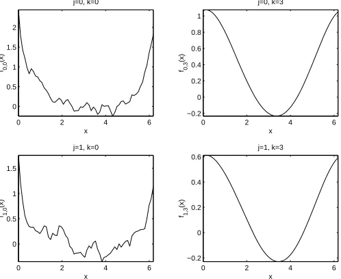
• We will make frequent use of a two-parameter family
of functions defined on the interval [0,2π]. First, we
define
f0
j,k(x) = Re
X
|ω|<N/2
ˆ
fj(1 +|ω|)−(k+1)eiωx
,
(58) forj, k= 0,1, . . . ,where
ˆ
fj(ω) =RjN+2(ω+N/2)−1+iRjN+2(ω+N/2). (59)
The parameterj indicates how many functions have
been generated in this fashion since setting MAT-LAB’s random number generator to its initial state,
and the parameterkindicates how smooth the
func-tion is. Figure 1 shows selected funcfunc-tions from this collection.
0 2 4 6
0 0.5 1 1.5 2
x
f0,0
(x)
j=0, k=0
0 2 4 6
−0.2 0 0.2 0.4 0.6 0.8 1
x
f0,3
(x)
j=0, k=3
0 2 4 6
0 0.5 1 1.5
x
f1,0
(x)
j=1, k=0
0 2 4 6
−0.2 0 0.2 0.4 0.6
x
f1,3
(x)
[image:11.595.309.554.266.464.2]j=1, k=3
Figure 1: Functions from the collection fj,k(x), for
se-lected values ofj andk.
In many cases, it is necessary to ensure that a func-tion is positive or negative, so we define the
transla-tion operatorsE+ andE− by
E+f(x) =f(x)− min
x∈[0,2π]f(x) + 1, (60)
E−f(x) =f(x)− max
x∈[0,2π]f(x)−1. (61)
• We define a similar two-parameter family of
func-tions defined on the rectangle [0,2π]×[0,2π]:
gj,k(x, y) = Re
X
|ω|,|ξ|<N/2
ˆ
gj(ω, ξ)ei(ωx+ξy)
,
(62)
wherej andkare nonnegative integers, and
ˆ
gj(ω, ξ) = (1 +|ω|)−(k+1)(1 +|ξ|)−(k+1)×
RjN2
+2[N(ω+N/2−1)+(ξ+N/2)]−1+
iRjN2
+2[N(ω+N/2−1)+(ξ+N/2)] .(63)
Figure 2 shows selected functions from this collec-tion.
0 2
4
0 2 4 0.05
0.1 0.15 0.2 0.25 0.3 0.35 0.4 0.45
x y
g0,3
(x,y)
j=0, k=3
0 2
4
0 2 4 −0.1
0 0.1 0.2 0.3 0.4 0.5 0.6
x y
g1,3
(x,y)
j=1, k=3
Figure 2: Functions from the collectiongj,k(x, y), for
se-lected values ofj andk.
In all experiments, unless otherwise noted, solutions
u(j)(x, t) are computed using time steps ∆t = 10·2−j,
for j = 0, . . . ,6. The error estimates are obtained by computing ku˜(j)(·,10)−u˜(6)(·,10)k
L2/ku˜(6)(·,1)kL2 for
j = 0, . . . ,5. This method of estimating error assumes
that u(6)(x, t) is a sufficiently accurate approximation to
the exact solution, but this has proven in practice to be a
valid assumption by comparingu(6) against approximate
solutions computed using established methods, and by
comparing u(6) against solutions obtained using various
methods with smaller time steps.
In [21], and in Section 6.3 of this paper, errors mea-sured by comparison to exact solutions of problems with source terms further validate the convergence behavior. It should be noted that we are not seeking a sharp esti-mate of the error, but rather an indication of the rate of
convergence, and for this goal, usingu(6) as an
[image:11.595.50.299.412.616.2]6.2
Smooth Coefficients
We now show the accuracy of our approach in one and two space dimensions. We solve the wave equation in which the spatial operator has a constant leading coef-ficient but a variable zero-order coefcoef-ficient, constructed from randomly generated Fourier coefficients as discussed in Section 6.1. Specifically, we solve the following prob-lems:
• ∂2u
∂t2(x, t)−
∂2u
∂x2(x, t)−E−f0,3(x)u(x, t) = 0, (64)
u(x,0) =E+f1,3(x), ut(x,0) =E+f2,3(x), (65)
u(x, t) =u(x+ 2π, t). (66)
• ∂u2
∂t2(x, y, t)−∆u(x, y, t)−E−g0,3(x, y)u(x, t) = 0,
(67)
u(x, y,0) =E+g1,3(x, y), ut(x, y,0) =E+g2,3,
(68)
u(x, y, t) =u(x+ 2π, t) =u(x, y+ 2π, t). (69)
In [21], it is shown that the methods for effi-ciently computing recursion coefficients generalizes in a straightforward manner to higher spatial dimen-sions.
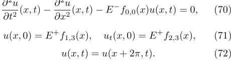
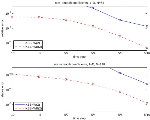
The results are shown in Figures 3 and 4, and Tables 1 and 2, and compared to those obtained using the original KSS method. In the 2-D case, the variable coefficient of the PDE is smoothed to a greater extent than in the 1-D case, because the prescribed decay rate of the Fourier
coefficients is imposed in both the x- and y-directions.
This results in greater accuracy in the 2-D case, which is consistent with the result proved in [20] that the lo-cal truncation error varies linearly with the variation in the coefficients. We see that significantly greater accu-racy is obtained with block KSS methods, especially in two space dimensions. Both methods exhibit sixth-order accuracy in time, consistent with the theoretical results proved earlier concerning local error.
In an attempt to understand why the block KSS method is significantly more accurate, we examine the
approx-imate solution operator for the simple case of K = 1.
As shown in (41), the original 1-node KSS method is equivalent to the simple splitting involving the averaged-coefficient operator. On the other hand, the 1-node block KSS method is not equivalent to such a splitting, because every node and weight of the quadrature rule used to com-pute each Fourier component is influenced by the solution from the previous time step.
Furthermore, an examination of the nodes for both meth-ods reveals that for the original KSS method, all of the
10 5 5/2 5/4 5/8 5/16
10−6 10−4
10−2
time step
relative error
smooth coefficients, 1−D, N=64
10 5 5/2 5/4 5/8 5/16
10−6
10−4
10−2
time step
relative error
smooth coefficients, 1−D, N=128 KSS−W(2)
KSS−WB(2)
KSS−W(2) KSS−WB(2)
Figure 3: (a) Top plot: Estimates of relative error in
the approximate solution of (64), (65), (66) at T = 10.
Solutions are computed using the original 2-node KSS method (solid curve), and a 2-node block KSS method
(dashed curve), both withN = 128 grid points. (b)
Bot-tom plot: Estimates of relative error in the approximate solution of the same problem, using the same methods,
with N = 256 grid points. In both cases, both methods
use time steps ∆t= 2−j, j= 0, . . . ,5.
nodes used to compute [ˆun+1]ω tend to be clustered
around ˆeHωLNˆeω, whereas with the block KSS method,
half of the nodes are clustered near this value, and the other half are clustered near [unω]HLNun
ω, so the previous
solution plays a much greater role in the construction of the quadrature rules.
A similar effect was achieved with the original KSS method by using a Gauss-Radau rule in which the pre-scribed node was an approximation of the smallest
eigen-value of LN, and while this significantly improved
ac-curacy for parabolic problems, as shown in [20], the solution-dependent approach used by the block method makes more sense, especially if the initial data happens to be oscillatory.
6.3
Oscillatory Coefficients
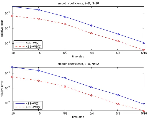
We now apply a 2-node block Krylov subspace spectral method to the problem
∂2u
∂t2(x, t)−
∂2u
∂x2(x, t)−E−f0,0(x)u(x, t) = 0, (70)
u(x,0) =E+f1,3(x), ut(x,0) =E+f2,3(x), (71)
u(x, t) =u(x+ 2π, t). (72)
[image:12.595.305.555.72.274.2] [image:12.595.320.550.658.720.2]Table 1: Estimates of relative error and temporal order of convergence in the approximate solution of (64), (65),
(66) at T = 10, using 2-node original and block Krylov
subspace spectral methods. Error is the relative differ-ence, in the 2-norm sense, between approximate solutions and a solution computed using a smaller time step, since
no exact solution is available. N denotes the number of
grid points and ∆t denotes the time step used.
N ∆t KSS-W(2) KSS-WB(2)
10 0.623 0.0844
5 0.0942 0.0466
64 2.5 0.00912 0.00142
1.25 0.000208 7.96e-005
0.625 3.41e-006 1.27e-006
0.3125 1.02e-007 1.81e-008
10 0.23 0.0404
5 0.0267 0.0169
128 2.5 0.0063 0.00127
1.25 0.000102 4.9e-005
0.625 2.37e-006 7.04e-007
[image:13.595.71.266.173.335.2]0.3125 5.29e-008 8.29e-009
Table 3 lists the relative errors for various time steps and grid sizes. The errors are obtained by comparing the approximate solution to the known exact solution in the 2-norm sense. While the performance of both methods are at least comparable in the case of smooth coefficients, KSS-W(2) exhibits severe instability for larger time steps, eventually recovering to achieve fourth-order convergence for smaller time steps. KSS-WB(2), on the other hand, while not as accurate as with smooth coefficients, still demonstrates fifth-order accuracy in time, and is stable
even for ∆t= 10. Unfortunately, some accuracy is lost as
the number of grid points increases. The error estimates are also plotted in Figure 5.
6.4
Variable Leading Coefficient and Source
Term
We will not prove stability for the 2-node case in this paper. Instead, we will provide numerical evidence of stability and a contrast with another high-order explicit method. In particular, we use the method KSS-W(2) to solve a second-order wave equation featuring a variable leading coefficient and a source term. First, we note that if p(x, t) andu(x, t) are solutions of the system of first-order wave equations
p u
t
=
0 a(x)
b(x) 0
p u
x
+
F G
, t≥0 (73)
with source terms F(x, t) and G(x, t), then u(x, t) also satisfies the second-order wave equation
∂2u
∂t2 =a(x)b(x)
∂2u
∂x2 +a′(x)b(x)
∂u
∂x +bFx+G (74)
10 5 5/2 5/4 5/8 5/16
10−8 10−5 10−2
time step
relative error
smooth coefficients, 2−D, N=16
10 5 5/2 5/4 5/8 5/16
10−8 10−5 10−2
time step
relative error
smooth coefficients, 2−D, N=32 KSS−W(2)
KSS−WB(2)
KSS−W(2) KSS−WB(2)
Figure 4: (a) Top plot: Estimates of relative error in
the approximate solution of (67), (68), (69) at T = 10.
Solutions are computed using the original 2-node KSS method (solid curve), and a 2-node block KSS method
(dashed curve), both with N = 16 grid points per
di-mension. (b) Bottom plot: Estimates of relative error in the approximate solution of the same problem, using the
same methods, withN = 32 grid points per dimension.
In both cases, both methods use time steps ∆t = 2−j,
j= 0, . . . ,5.
with the source term b(x)Fx(x, t) +G(x, t). In [13], a time-compact fourth-order finite-difference scheme is ap-plied to a problem of the form (73), with
F(x, t) = (a(x)−α2) sin(x−αt), G(x, t) = α(1−b(x)) sin(x−αt),
a(x) = 1 + 0.1 sinx, b(x) = 1,
which has the exact solutions
p(x, t) = −αcos(x−αt), u(x, t) = cos(x−αt).
We convert this problem to the form (74) and solve it with initial data
u(x,0) = cosx, (75)
ut(x,0) = sinx. (76)
The results of applying both methods to this problem
are shown in Figure 6, for the case α = 1. Due to the
[image:13.595.69.265.173.331.2]Table 2: Estimates of relative error and temporal order of convergence in the approximate solution of (67), (68),
(69) at T = 10, using 2-node original and block Krylov
subspace spectral methods. Error is the relative differ-ence, in the 2-norm sense, between approximate solutions
and a solution computed using a smaller time step. N
de-notes the number of grid points per dimension, and ∆t
denotes the time step used.
N ∆t KSS-W(2) KSS-WB(2)
10 0.207 0.00283
5 0.0479 0.000778
16 2.5 0.00207 7.12e-005
1.25 3.6e-005 1e-006
0.625 7.54e-007 2.99e-008
0.3125 1.35e-008 4.37e-010
10 0.168 0.0018
5 0.0357 0.000311
32 2.5 0.000993 2.08e-005
1.25 1.51e-005 3.34e-007
0.625 4.32e-007 6.76e-009
0.3125 5.49e-009 2.58e-010
The source term is handled by applying Duhamel’s prin-ciple, with a 4-node Gaussian rule over each time step, as first described in [21]. This has the effect of reducing
the average time step to ∆t/5 (in general, ∆5/(M + 1)
for an M-node Gaussian rule over each time step). For
[image:14.595.77.263.175.333.2]a more informative comparison, we therefore use this re-duced average time step in reporting the results for KSS methods.
Table 4 illustrates the differences in stability between the two methods. For the fourth-order finite-difference scheme from [13], the greatest accuracy is achieved for
cmax∆t/∆x close to the CFL limit of 1, where cmax =
maxx
p
a(x)b(x). However, for W(2) and
KSS-WB(2), this limit can be greatly exceeded and reasonable accuracy can still be achieved. In fact, while the results
reported here were obtained using N = 64 grid points,
nearly identical results are also obtained from substantial
increase in the number of grid points, such as N = 256,
with the same time steps.
7
Discussion
In this concluding section, we consider various general-izations of the problems and methods considered in this paper.
7.1
Higher Space Dimension
In [21], it is demonstrated how to compute the
recur-sion coefficients αj and βj for operators of the form
Lu=−p∆u+q(x, y)u, and the expressions are
straight-forward generalizations of the expressions for the
10 5 5/2 5/4 5/8 5/16
10−5 10−3 10−1
time step
relative error
non−smooth coefficients, 1−D, N=64
10 5 5/2 5/4 5/8 5/16
10−5 10−3 10−1
time step
relative error
non−smooth coefficients, 1−D, N=128 KSS−W(2)
KSS−WB(2)
KSS−W(2) KSS−WB(2)
Figure 5: (a) Top plot: Estimates of relative error in the
approximate solution of (70), (71), (72) atT = 10.
Solu-tions are computed using the original 2-node KSS method (solid curve), and a 2-node block KSS method (dashed
curve). Both methods use N = 128 grid points. (b)
Bottom plot: Estimates of relative error in the
approxi-mate solution of the same problem atT = 10. Solutions
are computed using the same methods, with N = 256
grid points. In both cases, both methods use time steps ∆t= 2−j,j= 0, . . . ,5.
dimensional case. It is therefore reasonable to suggest that for operators of this form, the consistency and sta-bility results given here for the one-dimensional case gen-eralize to higher dimensions. This will be investigated in the near future.
7.2
Discontinuous Coefficients and Data
As shown in [21] and again in the previous section of this paper, rough or discontinuous coefficients reduce the accuracy of KSS methods, because they introduce signif-icant spatial discretization error into the computation of recursion coefficients.
Furthermore, for the stability result reported in this pa-per, the assumption that the coefficients are bandlimited is crucial. It can be weakened to some extent and replaced by an appropriate assumption about the regularity of the coefficients, but for simplicity that was not pursued here.
Regardless, this result does not apply to problems in which the coefficients are discontinuous, because Gibbs’ phenomenon prevents their discrete Fourier transforms
from being uniformly bounded for allN. Similar
[image:14.595.77.262.175.334.2]Table 3: Estimates of relative error and temporal or-der of convergence in the approximate solution of (70), (71), (72) using 2-node original and block Krylov
sub-space spectral methods. Error is the relative
differ-ence, in the 2-norm sense, between the exact solution
u(x, t) = cos(x−t) and the computed solution atT = 10.
N denotes the number of grid points and ∆tdenotes the
time step used.
N ∆t KSS-W(2) KSS-WB(2)
10 4.64 0.0334
5 490 0.031
64 2.5 7.39 0.0144
1.25 0.517 0.00187
0.625 0.0129 8.44e-005
0.3125 0.00181 2.32e-006
10 17.7 0.14
5 4.04e+058 0.0622
128 2.5 4.56e+009 0.0259
1.25 12.7 0.00557
0.625 0.192 0.000558
[image:15.595.73.265.174.334.2]0.3125 0.00662 1.58e-005
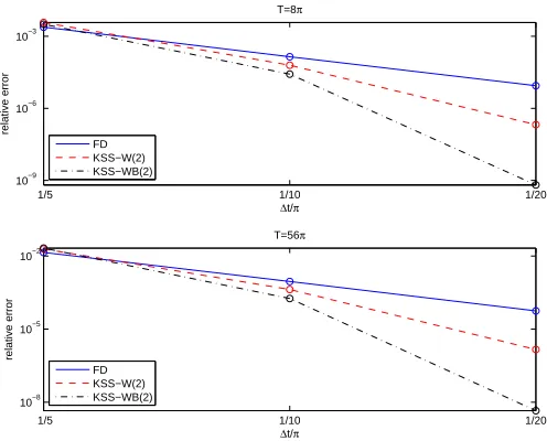
Table 4: Relative error in the solution of (74) with the time-compact fourth-order finite difference scheme from
[13], for various values ofN, and the KSS methods
KSS-W(2) and KSS-WB(2).
T ∆t FD KSS-W(2) KSS-WB(2)
0.62832 0.0024 0.00377 0.00318
8π 0.31416 0.00014 6.26e-005 2.67e-005
0.15708 8.8e-006 2.09e-007 6.52e-010
0.62832 0.014 0.0195 0.0211
56π 0.31416 0.0009 0.000423 0.00018
0.15708 5.6e-005 1.46e-006 4.5e-009
Ongoing work, described in [19], involves the use of the polar decomposition (42), to alleviate difficulties caused by such coefficients and initial data; future work will ex-plore possible combinations of this approach with block KSS methods in order to generalize the superior accuracy of the block approach to these more difficult problems.
7.3
Other
Boundary
Conditions
and
Maxwell’s Equations
While we only considered periodic boundary conditions in this paper, KSS methods for the wave equation can be used with other boundary conditions. Dirichlet bound-ary conditions were used in [12]. Inhomogeneous Dirich-let or Neumann boundary conditions can be handled by the standard technique of subtracting from the solution a function that satisfies the boundary conditions, and solv-ing a modified problem with an appropriate source term. Future work will explore the adaptation of KSS methods
1/5 1/10 1/20
10−9 10−6 10−3
∆t/π
relative error
T=8π
1/5 1/10 1/20
10−8 10−5 10−2
∆t/π
relative error
T=56π
FD KSS−W(2) KSS−WB(2)
FD KSS−W(2) KSS−WB(2)
Figure 6: Estimates of relative error in the approxi-mate solution of problem (74), (75), (76) with periodic
boundary conditions, at t = 8π (top plot) and t = 56π
(bottom plot), computed with the time-compact fourth-order finite-difference scheme from [13] (solid curve), a non-block KSS method (dashed curve), and a block KSS method (dotted-dashed curve). In the finite-difference
scheme, λ= ∆t/∆x= 0.99, and in both KSS methods,
2-point Gaussian quadrature rules are used, andN= 64
grid points.
for Maxwell’s equations, including the use of boundary conditions such as perfectly matched layers (PML), in-troduced by Berenger in [3], which can be implemented
by modifying the symbol ofLduring the computation of
the recursion coefficients, although they must be imple-mented carefully in view of the recent analysis of PML for variable-coefficient problems in [22].
7.4
Summary
We have demonstrated that for hyperbolic variable-coefficient PDE, block KSS methods are capable of com-puting Fourier components of the solution with greater accuracy than the original KSS methods, and they pos-sess similar stability properties in the case of smooth co-efficients, but are much more stable for problems with oscillatory coefficients. By pairing the solution from the previous time step with each trial function in a block and applying the Lanczos algorithm to them together, we obtain a block Gaussian quadrature rule that is better suited to approximating a bilinear form involving both functions than the approach of perturbing Krylov sub-spaces in the direction of the solution.
References
[1] Atkinson, K.: An Introduction to Numerical
[image:15.595.47.290.412.501.2][2] Basu, S., Bose, N. K.: Matrix Stieltjes series and
network models.SIAM J. Math. Anal.14(2) (1983)
209-222.
[3] Berenger, J,: A perfectly matched layer for the
ab-sorption of electromagnetic waves. J. Comp. Phys.
114(1994) 185-200.
[4] Dahlquist, G., Eisenstat, S. C., Golub, G. H.: Bounds for the error of linear systems of equations
using the theory of moments. J. Math. Anal. Appl.
37(1972) 151-166.
[5] Golub, G. H.: Some modified matrix eigenvalue
problems.SIAM Review15(1973) 318-334.
[6] Golub, G. H.: Bounds for matrix moments. Rocky
Mnt. J. of Math.4(1974) 207-211.
[7] Golub, G. H., Meurant, G.: Matrices, Moments and
Quadrature.Proceedings of the 15th Dundee
Confer-ence, June-July 1993, Griffiths, D. F., Watson, G. A. (eds.), Longman Scientific & Technical (1994)
[8] Golub, G. H., Gutknecht, M. H.: Modified Moments
for Indefinite Weight Functions.Numerische
Mathe-matik57(1989) 607-624.
[9] Golub G. H., van Loan, C. F.:Matrix Computations,
3rd Ed.Johns Hopkins University Press (1996)
[10] Golub, G. H., Underwood, R.: The block
Lanc-zos method for computing eigenvalues.Mathematical
Software III, J. Rice Ed., (1977) 361-377.
[11] Golub, G. H, Welsch, J.: Calculation of Gauss
Quadrature Rules.Math. Comp.23(1969) 221-230.
[12] Guidotti, P., Lambers, J. V., Sølna, K.: Analysis of 1-D Wave Propagation in Inhomogeneous Media. Numerical Functional Analysis and Optimization27
(2006) 25-55.
[13] Gustafsson, B., Mossberg, E.: Time Compact High Order Difference Methods for Wave Propagation. SIAM J. Sci. Comput.26(2004) 259-271.
[14] Hochbruck, M., Lubich, C.: On Krylov Subspace Approximations to the Matrix Exponential Opera-tor.SIAM Journal of Numerical Analysis34(1996) 1911-1925.
[15] Lambers, J. V.: Derivation of High-Order Spec-tral Methods for Time-dependent PDE using
Modi-fied Moments.Electronic Transactions on Numerical
Analysis28(2008) 114-135.
[16] Lambers, J. V.: Enhancement of Krylov
Sub-space Spectral Methods by Block Lanczos Iteration. Electronic Transactions on Numerical Analysis 31
(2008) in press.
[17] Lambers, J. V.: Implicitly Defined High-Order
Operator Splittings for Parabolic and Hyperbolic Variable-Coefficient PDE Using Modified Moments. International Journal of Computational Science 2
(2008) 376-401.
[18] Lambers, J. V.: Krylov Subspace Methods for
Variable-Coefficient Initial-Boundary Value Prob-lems. Ph.D. Thesis, Stanford University, SCCM Pro-gram, 2003.
[19] Lambers, J. V.: Krylov Subspace Spectral Methods
for the Time-Dependent Schr¨odinger Equation with
Non-Smooth Potentials. Submitted.
[20] Lambers, J. V.: Krylov Subspace Spectral Meth-ods for Variable-Coefficient Initial-Boundary Value
Problems. Electronic Transactions on Numerical
Analysis20(2005) 212-234.
[21] Lambers, J. V.: Practical Implementation of Krylov
Subspace Spectral Methods. Journal of Scientific
Computing32(2007) 449-476.
[22] Oskooi, A. F., Zhang, L., Avniel, Y., and Johnson, S. G.: The failure of perfectly matched layers, and towards their redemption by adiabatic absorbers. Opt. Expr.16(2008) 11376-11392.
[23] Shampine, L. F., Reichelt, M. W.: The MATLAB
ODE suite. SIAM Journal of Scientific Computing
18(1997) 1-22.
[24] Stoer, J., Burlisch, R.: Introduction to numerical