Pilot Plant Batch Distillation pdf

(1)

See also: I/Distillation: Historical Development; Model-ling and Simulation; Theory of Distillation; Tray Columns: Performance; Tray Columns: Performance; Vapour-Liquid Equilibrium; Correlation and Prediction; Vapour-Liquid Equilibrium: Theory.

Pilot Plant Batch Distillation

M. A. P. de Carvalho and

W. R. Curtis, The Pennsylvania State University, PA, USA

Introduction

Laboratory distillation encompasses an operating range from millilitres in bench-top devices to pilot units with the capacity for producing several hundred kilograms of product per day. While the design of bench-top assemblies is generally geared towards the achievement of a speciRed purity grade of the desired product, quantitative predictions are not usually feas-ible for such equipment and their construction relies a great deal on ingenuity and craftsmanship. For dedicated applications, glassware companies offer off-the-shelf equipment. This article will therefore focus on the pilot-scale units, where the analytical principles of mass and heat transfer can be applied to the operation, design and optimization of the equipment.

The section on theory presents analytical descrip-tions of batch distillation for three different ap-proaches in order of decreasing complexity. It starts with a comprehensive model for a nonadiabatic, non-zero hold-up, nonconstant molar overSow, nonideal multicomponent column. The second model present-ed neglects stage hold-ups and assumes adiabatic stages and constant molar over_Sows to arrive at a set of equations describing the transient behaviour of the equipment, which can be solved for a binary system using a simple spreadsheet. If constant relative vola-tility and operation at minimum reSux are further

assumed, the derivation of a third model is possible, where the transient states within the equipment are given by direct analytical expressions.

The design of a batch column can be a challenging task because batch distillation presents unique con-siderations that are not addressed in most of the available literature, which is concerned with continu-ous operation. The section on design is a collection of advice and criteria for the design of batch columns. SpeciRc information is given about equip-ment for batch distillation and accompanying instru-mentation and safety circuitry. Details are drawn from a pilot-scale column that is installed in Penn State University’s Department of Chemical Engineer-ing. The section on column operation extends the scope of the two preceding sections by providing information on establishing operating strategies and operating protocols for batch runs. Much of this information is based on hands-on experience ac-quired with the column described in the subsection on equipment.

(2)

[image:2.568.301.499.57.396.2]

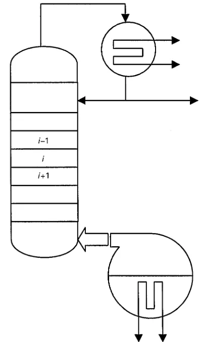
Figure 1 Batch distillation column schematic for a rectifying configuration.

providing references for those interested in further reading.

Theory

The theory of batch distillation permits design, opera-tion and optimizaopera-tion calculaopera-tions by integrating the concepts of thermodynamic equilibrium, mass and heat transfer, energy and material balances to solve the problem of predicting the compositions and_Sow rates of process streams. The traditional approach to the development of governing equations is to model the equipment as a stack of equilibrium stages. De-partures from ideality are taken into account by in-troducing the concept of stage efRciencies. Modelling in terms of equilibrium stages is convenient because of the availability of extensive equilibrium data for multicomponent systems and the associated predic-tive thermodynamic models. Packed columns, which do not possess physical mass transfer stages, can be translated into this technical framework by the use of the transfer unit concept (see, for example, McCabe

et al., 1993).

Relinquishing or including levels of complexity and interdependence in the fundamental equation and process variables will result in more or less rigorous treatments, with gains in accuracy usually being ac-companied by substantial drawbacks in complexity and computational difRculty. Hereunder, three differ-ent sets of model equations are presdiffer-ented in decreas-ing levels of complexity. A rigorous approach to the problem involves the solution of a set of time-depen-dent differential and algebraic equations for the ma-terial and heat balances and for the equilibrium rela-tions. Batch columns are usually constructed so that there is only one section, either above or below the feed stage. The typical column design depicted in Figure 1 represents the rectifying section. From this simpli_Rcation it is possible to write the following equations to de_Rne the problem completely in each stage except the top stage and the feed drum (re-boiler).

Total material balance

dhL tot,i

dt "Li\1#Vi#1!Li!Vi [1]

Component material balances

hL tot,i

dxi,j

dt"Li\1xi\1,j#Vi#1yi#1,j!Lixi,j!Viyi,j

i"1,Nstage,j"1,NC [2]

Energy balance

hL

tot,i NC

x"1 xi,j

dHL i,j

dT

dt"Li\1xi\1,jH L i_\1,j

#Vi#1yi#1,jHVi#1,j

!Lixi,jHLi,j!Viyi,jHVi,j#Qi

i"1,Nstage,j"1,NC [3]

Vapour liquid equilibrium relation

yi,j"f(xi,j) [4]

Summation of liquid mole fractions

NC

j"1

xi,j"1 [5]

Summation of vapour mole fractions

NC

j"1

(3)

Liquid total hold-up constraint

hL tot,i

NC

j"1

xi,jvj

"Vol [7]

Eqns [1]}[7] ignore the tray hydraulic behaviour

and assume identical compositions for the liquid hold-up within a stage and the liquid out_Sow out of the stage. Other major features and assumptions of the model are nonadiabatic stages, negligible vapour hold-up and constant volumetric liquid hold-up. The assumptions concerning the hold-up are very reason-able and the equations can be readily translated to real stages by the introduction of Murphree tray

ef-Rciencies as correction factors for either the liquid or the vapour compositions.

For the top stage, the liquid inSow is related to the distillate outSow by the reSux ratio, and for the feed drum, the depletion of material should be taken into account. There is also no liquid outSow for the re-boiler, thereby decreasing the number of necessary equations by one (eqn [7]). The following equations are the modi_Red set for the situation in the top stage and reboiler.

Top stage: total material balance

dhL tot,1

dt "DRD#V2!L1!V1 [8]

Component material balances

hL tot,1

dx1,j

dt "DRDxD,j#V2y2,j!L1x1,j!V1y1,j [9]

Energy balance

hL

tot,1 NC

x"1 x1,jHL1,j

dHL 1,j

dT

dT dt

"DRDxD,jHLD,j#V2y2,jHV2,j!L1xi,jHL1,j

!V1y1,jHV1,j#Q1 [10]

For the feed drum (reboiler) the following equa-tions are modiRed.

Total material balance

dhL tot,R

dt "LN stage!VR [11]

Component material balances

hL tot, R

dxR,j

dt "LN stagexN stage,j!VRyR,j [12]

Energy balance

hL

tot,R NC

x"1 xR,jHLR,j

dHL R,j

dT

dT dt

"LN stagexN stage,jHLN stage,j!VRyR,jHVR,j#QR [13]

The set of equations written for all the stages forms a system of nonlinear differential algebraic equations, with initial conditions given by the original charge in the feed drum, tray hold-ups and tray composition proRles and internalSow rates. The vector of initial conditions represents a pseudo steady-state solution for an initial feed whose composition is equal to the vapour in equilibrium with the liquid charge of the feed vessel. The transient behaviour is obtained by the simultaneous solution of eqns [1]}[13], which

re-quires linearization and a combination of matrix in-version and integration techniques.

Despite the large range of computational complex-ity, simulations of batch distillation show that, in most cases, short-cut and rigorous models agree very well. A distinct advantage of the simpliRed models is they can be implemented in a spreadsheet. In these models the stage hold-up is considered negligible, except for the feed drum (reboiler) where the

following equations hold for the total and

volatile component material balances in a column operating at constant distillate composition and vari-able reSux.

Total cumulative material balance

D_M _"V_M _!L_M [14]

dW"!dDM "

1!LM

VM

dVM "

1! R R#1

dVM

"(1!S)dVM [15]

Cumulative component balance

Wixwi"Wxw#(Wi!W)xD [16]

By differentiating and rearranging one gets:

W"Wi(xwi!xD)

(xw!xD)

[17]

!dW"Wi(xD!xwi)dxw

(xD!xw)2 "

(4)

[image:4.568.134.434.506.697.2]

Figure 2 Optimum profit profile: operating costs versus length of time. Recovered product increases rapidly at first but then levels off.

If eqn [18] is substituted in [15] one gets:

(1!S)dVM"Wi(xD!xwi)dxw

(xD!xw)2

[19]

The total amount of vapour produced will then be:

VM"

xwf

xwi

Wi(xD!xwi)

(1!S)

dxw

(xD!xw)2

[20]

Since the cumulative vapour produced is VM "V, the timenecessary for a run is calculated from the above equation as:

"

xwf

xwi

Wi(xD!xwi)

V

dxw

(1!S) (xD!xw)2

[21]

The total amount of distillate produced can be found by integration of eqn [18]:

Df

0

dDM "

xwf

xwi

Wi(xD!xwi)dxw

(xD!xw)2

[22]

Finally, rearrangement of eqn [16] yields:

Wixwi!(Wi!W)xD"Wxw [23]

Wixwi!DM xD"Wxw [24]

The above can be differentiated to give the follow-ing result:

d(Wixwi!DM xD)"d(Wxw) [25]

!d(DM xD)"d(Wxw) [26]

!xDdDM "xwdW#Wdxw [27]

The remaining amount of charge in the still is then calculated by combining the above equation with the total differential balance dW"!dDM and sub-sequently integrating the resultant expression:

dW W"

dxw xD!xw

[28]

lnWf

Wi

"

xwf

xwi dxw xD!xw

[29]

Eqns [20]}[22] provide an efRcient way of

calcu-lating the total amounts of vapour and distillate pro-duced and the time necessary for the separation with-out having to solve the system of equations comprised by eqns [1]}[13]. This calculation provides an

eco-nomic benchmark since it deRnes the optimum time for a run, based on the recovered product value and the operating costs. As the run time increases, the cumulative revenues given by the total amount of recovered product multiplied by its value will Rrst increase but then approach an asymptotic value. The decreased economic bene_Rt results either because the amount of distillate decreases (as in the case of con-stant composition distillate) or because the product stream becomes progressively less pure (as in the case of constant reSux ratio operation). The operating costs on the other hand increase steadily with time and the proRt function, which combines these two costs, undergoes a maximum, after which the proRt will decrease, as illustrated byFigure 2.

(5)

line. The slope of the operating line is then given by:

S"dLM dVM"

xD!yw xD!xw"

R

R#1 [30]

Under the constraint of constant relative volatility the equilibrium relation becomes:

yw"

xw

1!xw(#1)

[31]

If one takes advantage of eqns [30] and [31], ana-lytical forms for the cumulative distillate production and remaining charge left in the feed still can be derived for the cases of either constant reSux ratio or constant distillate composition operation.

For constant reSux ratio, eqn [15] can be inte-grated to the expression for the total vapour require-ment:

VM"(R#1)DM "(R#1) (Wi!Wf) [32]

Combination of eqns [15], [30] and [31] yields the functional dependence of distillate composition,

xD on recycle ratio,R, composition of the remaining

feed,xwin the reboiler and relative volatility, :

xD"

(R#1)xw!Rxw!Rx2w(!1)

1#xw(!1)

[33]

Substitution of eqn [33] into the general mass bal-ance expression, eqn [29] and subsequent integration produces an analytical form for the mass balance given by:

lnWf

Wi

" 1

(R#1) (!1)ln

1!xwi

1!xwf

xwf xwi

#

1

R#1

ln

1!xwf

1!xwi

[34]

If the column is operated at constant distillate com-position, direct integration of eqn [29] produces the expression for the mass balance:

Wf Wi

"

xD!xwi xD!xwf

[35]

The integration of eqn [20], however, requires the development of an expression for the time-dependent operating line, which is accomplished by substitution

of eqn [31] into [30] to yield:

dLM dVM "

xD#xDxw(!1)!xw

(xD!xw) [1#xw(!1)]

[36]

Substitution of [36] into the general expression for the vapour requirement (eqn [20]) and integration leads to the vapour requirement equation when the column is operated at constant distillate composition and variable reSux:

VM" Wi(xD!xwi)

(1!xD) (xD) (!1)

;

(1!xD) ln

xD!xwf xD!xwi

#

xwi xwf

#xDln

xD!xwf xD!xwi

1!xwi

1!xwf

[37]

Eqns [34] and [37] were developed by Bauerle and Sandall, assuming the ideal pinched columns operat-ing at minimum reSux. None the less, their applica-tion to real columns yields good approximated results if the equipment operates in a near-pinched zone at the bottom. This is often the case for columns with

Rve or more theoretical stages.

Design

The operation of a batch distillation column, even pilot-scale equipment, is often as technically involved as operation of an industrial-scale column, and the same amount of care in start-up and safety proced-ures should be taken. Whether designing a new col-umn or revamping an existing one, the necessary safety and physical properties data such as_Sash and ignition points, _Sammability and toxicity must be compiled for each component in the mixture. Predic-tive equations or experimental values for the vapour pressures of all components and binary equilibrium data should be compiled together with parameters of equations of state or activity coefRcient models when-ever available. Other physical properties to be in-cluded are liquid and vapour heat capacities, heats of vaporization and viscosities.

Once the physical property data bank has been put together, preliminary design calculations can be per-formed. For a multicomponent distillation column a light-key and a heavy-key component should be chosen in order to reduce the preliminary design to a pseudo-binary system. At this point it is possible to use graphical methods like McCabe}Thiele or even

(6)

carry our a case study toRnd out the system response in terms of required number of theoretical stages for a speciRed purity at different reSux ratios. To accom-plish this, the optimization techniques described later can be useful, but since they are also hard to imple-ment. The alternative approach of using a simpliRed calculation method such as presented in the section on column operation might be more desirable. This initial set (reSux ratio!number of theoretical stages) will permit the preliminary design.

Depending on the intended purpose of the laborat-ory-scale column, these initial calculations are likely to be sufRcient for specifying the details of column design. Reboiler and condenser heat loads permit sizing of steam and condensation coils. Environ-mental concerns have introduced complexities in de-sign which were not previously an issue for pilot-scale distillation. Current regulations at our site require condensate return to steam generation facilities to recover waste heat. Even a moderate condenser heat load can require prohibitively large quantities of cold tap water and the condenser heat load for even a small distillation column will typically be substan-tially larger than can be handled by laboratory-scale recirculated chillers. Much of the _Rnal decisions on absolute sizing will be dependent upon available fa-cilities and the anticipated intensity of column use. It is important to get to a reasonably accurate prelimi-nary design early in the design process, so that such practical constraints can be considered.

In many situations, a laboratory-scale distillation column will be used for multiple separations, or as a testing ground for additional full-scale design data. Under these circumstances, design for Sexibility is a primary concern. Instead of focusing on detailed physical property information, the data collection should focus on obtaining ranges of anticipated phys-ical properties as well as ranges in batch size. The actual design should then re_Sect the appropriate bounds of properties and separations that may be encountered. It should be kept in mind that there is a practical minimum volume that can be handled, due to tray hold-up, while larger volumes can be handled with multiple batches. Undersizing either reboiler or condenser heat transfer capacity may render the col-umn useless for a speciRc separation.

In most batch distillation operations, the lighter component is the desired product and the actual col-umn is the rectifying section of a continuous tower. The preceding discussion in this section as well as in the next section implicitly assume this situation. Nevertheless, there might arise design situations where the economical interest lies in the heavier com-pounds. In more complex operations the designer might even be faced with the task of devising a

separ-ation sequence involving two or more columns. For the case where it is desired to recover the heavy component, the calculations for the number of stages should be performed as a stripping column instead.

Since the principles and computational basis of distillation are quite advanced, additional assump-tions allow the derivation of simple expressions for

the distillate composition and Sow rate and the

amount of material left in the feed drum. These as-sumptions render the evaluation of columns with recycle amenable to straightforward solutions.

The remainder of this section includes a description of a versatile laboratory distillation column and its instrumentation and safety systems.

Equipment

Batch distillation equipment can be custom-made to meet particular design speciRcations or be directly purchased by catalogue selection if no stringent con-struction features or materials are required. Ordering can be greatly facilitated by a previous search of the manufacturers or suppliers in the worldwide web. Equipment intended to be used for research or educa-tional purposes should be made of glass whenever possible, given the easy observation of the internal

Sow regimes and their change with the internalSow rates. An existing batch glass column is described here as an example.

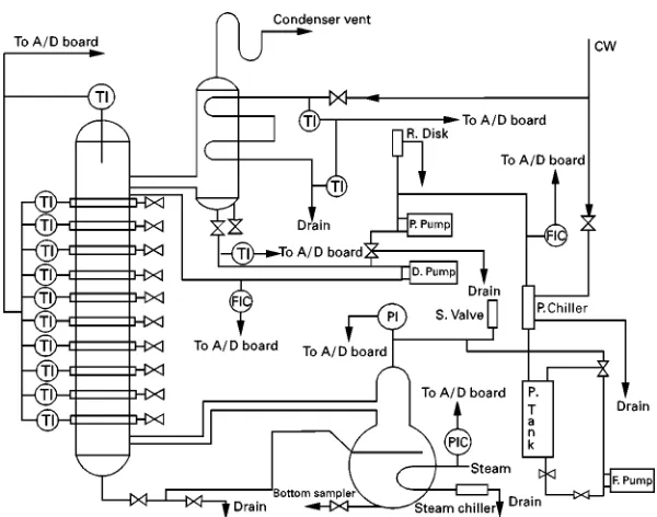
Figure 3 shows a distillation column which has a simple conceptual design but is versatile enough to be used for research or teaching applications. The column is atmospheric and functions as the rectifying section of a regular distillation column. The feed drum doubles as a kettle vessel where the feed is vaporized by a coil heater having steam as the heating medium. Instrumentation is reduced to the essentials: the distillate and re_Sux_Sow rates are controlled by varying the rotation speed of the distillate and re_Sex pumps, and the feedSow rate can be controlled by varying the steam pressure in the coil. The safety system consists of a relay actuated by the occurrence of any of the failure conditions in the column, which are pressurization within the equipment, zeroSow of condenser cooling water or loss of power to the ventilation system. When any of these conditions occurs, steam admission to the feed drum is switched off.

(7)

[image:7.568.135.435.53.289.2]

Figure 3 Rectifying batch distillation column. The abbreviations are as follows: A/D board"analog to digital interface board, CW"cooling water, D. Pump"distillate pump, F. Pump"feed pump, FIC"flow indicator control, P. chiller"product chiller, P. Tank"product tank, PI"pressure indicator, PIC"pressure indicator control, R. Disk"rupture disk, S. Valve"safety valve and TI"temperature indicator.

a software utility provided with the board that emu-lates a control panel, where each of the instruments hooked to the board is assigned a channel number displayed in the panel screen. The user varies the pumpSow rate by changing the output current at the computer screen. Manual local control of each pump is also provided in case of failure of the computer-interfaced control. The stepper motor of the steam valve for the feed drum steam coil is also interfaced in a comparable manner.

The column is also provided with thermocouples for each stage, including condenser and reboiler. The thermocouples are wired to a screw terminal connec-tor, that provides the interface to an analog_/digital I_/O board installed in the PC. When there is a signi_R -cant difference between the boiling points of the two components of a binary system, the stage temperature is an efRcient and straightforward way of evaluating compositions. Under these circumstances, the real-time composition proRle within the column can be updated to the computer screen. Sample ports for the liquid phase are installed in every stage, including the condenser and reboiler to corroborate thermal measurements under circumstances where thermal gradients are not sufRciently steep to provide accurate composition correlation. The composition analysis can be performed by a variety of methods. If there is a signi_Rcant density difference between components being separated, composition can be deduced from a density}concentration curve. Density can be

deter-mined gravimetrically, or equipment is available for online density measurement. A particularly versatile online implementation of density measurement is in the condensate stream of an off-set condenser as described in more detail below. If one of the compo-nents is an organic acid, sample analysis can be car-ried out either by titration or by the measurement of any other property related to the dissociation state (such as pH), provided the metering apparatus is sufRciently accurate to discriminate stage-to-stage differences. For organic mixtures, other properties such as refractive index may also be used as analytical method.

The feed drum in the described pilot-scale column is a large glass bulb equipped with a steam heating coil to vaporize the feed. A pressure relief rupture disk provides a mechanical fail-safe against reboiler pressurization. Another pressure gauge is installed at the steam inlet to the coil. The steam outlet is pro-vided with a trap to ensure the total condensation of the steam, and therefore the use of its latent heat. A useful energy balance is achieved by cooling the condensate as it is discharged to the drain. The heat load to the column can be crudely calculated by

measuring the discharge Sow rate and multiplying

this valve by the heat of vaporization of the steam at the inlet pressure.

(8)

charging of material to the feed drum. The remaining material in the drum after a batch processing can be discharged by a valve in the bottom. The subsequent batch charge can also be combined with the remain-ing heavy ends of the previous operation.

The off-set condenser depicted in Figure 3 provides for direct measurement of condensateSow rate. This eliminates the need to calculate condensate from the condenser energy balance. This is particularly impor-tant for pilot-scale units where complete condensa-tion may not be achieved at high boil-up rates. The condensed top vapours drip down and accumulate in the bottom part of the vessel, from which they are removed either to the distillate tank or back to the column as reSux. A match between the condensation rate and sum of product and liquidSow rate returned to the column can be assured by visual monitoring of the condenser liquid level or computer monitoring of the liquid head in the bottom of the condenser with a pressure transducer. The gas entrance to the con-denser doubles as a liquid overSow in the event of excessive condensate accumulation.

Instrumentation and Safety Circuits

Although a batch distillation column can be run man-ually by an attentive and experienced technician, the dynamic nature of operation requires extensive in-strumentation for all but the simplest mode of opera-tion. To gain theSexibility necessary for the opera-tion at constant distillate composiopera-tion,Sow rates of the reSux and distillate must be independently con-trolled. In small units devoted to research,Sow con-trol can be easily accomplished by varying the speed of a gear pump through a control panel displayed on a computer screen. The connection of the pump to the computer consists of a driver board wired to a screw terminal connector. The latter is attached to an ana-log output board. The output signal to the driver board can be varied based on the results of calcu-lations performed by external application programs. If the top composition is to be kept constant, the update on the reSux rate can be calculated by a user routine with the aid of operating charts such as those described later. The value of the reSux rate translated to Sow rates (typically current values) controls the distillate and reSux pumps. The product and reSux

Sow rates must be constrained to balance the rate of condensation. This is conveniently accomplished by monitoring the condenser level as an indicator of the difference between boil-up and distillate and product

Sow rates. The direct use of the heat load output to control the condenser level is not recommended due to the large dead-time between a change in the re-boiler conditions and the resulting effect in the liquid

level. The result of the reSux calculation is stored in a data buffer from which it can be retrieved by an-other application and used to update the correspond-ing analog output channel.

Analog and digital I/O boards can also be installed to retrieve information such as cooling water temper-ature andSow rate, steam pressure,Sow rate to the reboiler and the temperature proRle of the column. The stage temperature is a direct indicator of stage composition; however, it is only useful as a control variable when the temperature variation between suc-cessive stages is signi_Rcant. The greatest variation in temperature during the batch run will take place in the reboiler which is an excellent means of monitor-ing overall progress of the separation.

Variation of the heat load to the column can be

actuated remotely by Rtting the steam valve with

a stepper motor. A variable heat load adds operation

Sexibility and can be used in conjunction with other strategies to maximize recovery and purity of a de-sired component at a lower energy cost. For example, the feed drum contains the highest fraction of the

volatile component at the beginning of the

process. Therefore, the column can be started up at a lower boil-up rate, which will be gradually increased to match the enrichment of the charge in the heavier component. Figure 3 shows typical column instrumentation, and data acquisition and control.

Three operating conditions are monitored con-stantly and may independently activate the safety system, stopping steam delivery to the reboiler by closing a steam safety valve that precedes the steam controller valve. These monitored conditions are the column pressure, cooling waterSow and ventilation fans. The pressure transducers,Sow transmitter and power to the fans are set up as a logic relay where loss of any one of the direct current voltages is suf_Rcient to actuate the steam safety valve. It is important to choose the logic of these circuits such that electrical and mechanical failures will default to termination of the batch run. The safety system circuitry is depicted inFigure 4.

Column Operation

(9)

[image:9.568.131.442.55.507.2]

Figure 4 Safety system circuitry.

accounted for in the calculation theory. A variety of operation and completion criteria may be used de-pending on the process economics, equipment charac-teristics and product value. Several different basic operational modes are possible:

1. total reSux, with periodic dumping of the accumu-lated material from the condenser to the distillate tank;

2. constant re_Sux, with continuous variation of the instantaneous distillate composition, starting

above and Rnishing below the desired product

speciRcation;

3. constant composition, with variable reSux ratio in order to keep the instantaneous distillate composi-tion constant.

Operation strategies can take advantage of all three of these operational modes.

(10)

[image:10.568.102.489.392.699.2]

Figure 5 Representation of stage efficiencies.

operation is switched to the constant reSux mode and continued until the average composition of the distil-late drops to the desired level, when the equipment is shut down. Variations on this approach are often required due to equipment limitations. If the column is to be operated manually, then it might be difRcult to maintain constant distillate composition. Also, if the column consists of less than Rve ideal stages, it is more advantageous to operate at constant re_Sux.

Prior to the initiation of any operational procedure, it is necessary to elaborate an operation schedule that can be used as a guide throughout the run. Although the procedures discussed here can be implemented for columns with a very low level of automation, they can also be used in application programs that run as a part of an automated control loop. One can use simpliRed calculation methods (e.g. McCabe}Thiele)

or resort to more extensive numerical computations if the effect of some variables such as the hold-up is to be taken into account. Independent of the calcu-lational basis, better predictions of the composition proRles can be obtained if the stage efRciencies or at least the overall ef_Rciency is known. Ef_Rciencies depend on the physical properties of the system, par-ticularly the viscosity and the relative volatility, but also on the geometric characteristics of the equip-ment. Determination of the overall and stage efR cien-cies can be easily accomplished by running the

col-umn at total reSux. When the column has reached

steady state, the composition proRles within the col-umn must be determined. The overall efRciency is easily calculated by stepping off theoretical stages in the McCabe}Thiele diagram between the equilibrium

and the operating line, which at total reSux coincides withy"x. The number of theoretical stages is deter-mined when the bottom composition is crossed. The Murphree efRciency for stagenreceiving liquid from stagen!1 and vapour from stagen#1 is deRned as:

M"

yn!yn_\1 yeq

n!yn_\1

[38]

Eqn [38] is a measure of the degree of separation

achieved in the vapour going from stage n#1 to

stagenand can be visualized in the McCabe}Thiele

diagram as a segment ratio, as shown inFigure 5. The maximum degree of separation is represented by the difference in the denominator, where the vapour leav-ing the stage is in equilibrium with the liquid phase of the same stage.

Determination of the vapour-phase composition is often more difRcult than liquid and sample ports are generally only provided for the liquid phase. It is therefore useful to de_Rne Murphree ef_Rciency of the liquid compositions as:

M"

xn#1!xn xn#1!xeqn

(11)

[image:11.568.165.391.513.682.2]

Figure 6 Operation schedule at constant composition. Reflux schedule (based on 45%overall).Xbis the reboiler composition,

Xdis the distillate composition andRdis the reflex ratio.

Once the efRciencies are determined, an operation schedule at constant reSux should be prepared. The operation schedule consists of a family of curves where the reSux ratio is plotted as a function of reboiler composition, holding the distillate composi-tion constant as depicted inFigure 6. The curves can easily be generated in a spreadsheet if the equilibrium curve for the system can be regressed as an analytical form,x"f(y). A distillate composition (xD) isRxed as

the fulcrum, around which all the operating lines pivot, as de_Rned for different re_Sux ratios (RD), as

shown inFigure 7. Since the number of ideal stages is known, the bottoms composition (xB) is found for

each operating line by stepping off these stages be-tween the equilibrium curve and the operating lines. OncexBis found for a particular operating line, the

reSux ratio is changed, thereby deRning another oper-ating line, and the procedure is repeated to Rnd the correspondingxB. In this way, a set of data points

(RD,xB) corresponding to a Rxed distillate

composi-tionxDis determined. The next set is determined by

the same procedure, changing the value ofxD. These

plots of RD versus xB represent the reSux ratio

re-quired to achieve a speci_Red distillate composition at a given composition within the reboiler.

The RD versus xB curves can either be used in

manual operation or integrated into an automated control strategy, where information about the feed drum composition is used to calculate the new re-quired reSux ratio to keepxDconstant. The choice of xDwill depend on the minimum acceptable purity for

the product. Sometimes, even when a higher purity is desired, the operatingxDmay be imposed by

equip-ment restrictions. TheSow rate range of the pumps, for example, might restrict operation to a certain range of the reSux ratio. In this case, switching to

a lower distillate composition will allow longer runs, thus increasing the total amount of product.

Stopping criteria for an industrial distillation is generally dictated by economics. Operating costs ac-cumulate continuously with time, because of energy and labour costs, as discussed above.

Optimization Techniques

Optimization of batch distillation operations is not addressed with the same frequency as the continuous-case counterpart. The likely reason for the scarcity of publications in this area lies in the transient nature of the problem, which introduces a system of differential equations to describe the dynamics. The optimization problem therefore consists of a target functional (see below) to be minimized and a set of constraints em-bodied by the differential equations for the time-dependent behaviour of material and energy balances and algebraic equations for phase equilibrium and column hydraulics plus additional constraints such as bounds on certain variables. Optimization problems with nonlinear algebraic model equations and con-straints can be solved in a straightforward way by nonlinear programming strategies. On the other hand, unconstrained problems with differential equa-tion models can be handled through the calculus of variations. Models that combine both of these fea-tures are currently optimized by imposing some level of approximation to the problem. The problems usu-ally reported in the literature for batch distillation can be classiRed as:

(12)

[image:12.568.56.277.54.260.2]

Figure 7 Construction of the operation schedule.

2. Minimum time problem: to minimize the batch time needed to produce a prescribed amount of distillate of a speci_Red purity.

3. Maximum pro_Rt problem: to maximize a pro_Rt

function for a speci_Red purity of distillate.

The maximum proRt problem for a column

oper-ated at constant distillate composition involves the evaluation of the net proRt of the column along its batch run time. The net proRt function behaviour has already been discussed. The proRt curve displays an extrema and the proRt optimization problem there-fore seeks the value of the batch run time (a number) that will maximize the net proRt function. It is amen-able to a simple graphic solution that can be obtained from a spreadsheet as long as a simple zero hold-up model is employed to describe the column operation. On the other hand, the solution of the maximum distillate problem is given by a time-dependent func-tion (the distillateSow rate) that will maximize the cumulative distillate production, a function of the distillate Sow rate. This latter function of another function is called a functional.

In this section some of the recently developed tech-niques to extremize functionals are brieSy reviewed. The objective is to offer the reader an introduction to the theme, and provide useful references for further information. The optimization problem belonging to one of the above categories can be posed in terms of an objective function subjected to constraints such as:

Min

u(t),z(t),p

"(z(b),p)#

b

a

G(z(t),u(t),p)dt [40]

subject to:

zR(t)"F(z(t),u(t),p) [41]

g(u(t),z(t))40 [42]

gf(z(b))40 [43]

z(a)"z0 [44]

z(t)L₄_z(t)₄_z(t)U _[45]

u(t)L₄_u(t)₄_u(t)U _[46]

In the above set of equations the integral part of the objective function to be minimized can be viewed as the total amount of distillate, withdrawn as top prod-uct, whereas the function(z(b),p) may account for theRnal hold-up within the equipment, which can be incorporated into the product at the end of a batch run. The vectorz(t) represents the state variables of the system, such as composition, internalSow rates and temperatures, and the vector p represents con-stant parameters. The vectoru(t) carries the control pro_Rles, i.e. the variables used to manipulate eqn [40] and achieve the minimization goal. Distillate of a spe-ciRed purity can be maximized for instance by chang-ing the reSux ratio. The time-dependent reSux ratio would be then the control variableu(t) for such an optimization problem. The constraints represented by eqn [41] embody the material and energy balances, which are written in their transient form for the batch problem. Algebraic constraints included in eqn [42] may represent the equilibrium relations and the sum-mation of the liquid mole fractions. Inequality con-straints with lower and upper bounds (eqns [45] and [46]) may represent either purity requirements in the product or physical constraints in the maximum and minimum attainable values of the control variables. Initial andRnal states of the system are also written as constraints, as represented by eqns [44] and [43] re-spectively.

(13)

represented by:

Min

u(t),z(t),p

1_"_(z(b),_p)_#T_gf(z(b))

#

b

a

[G(z(t),u(t),p)

# T_(t)(F(z(t),_u(t),_p)_!_z_(t))

#MT_(t)(g(u(t),_z(t))_#_s2_)]_dt _[47]

By analogy to Hamilton’s equation of motion, one can deRne a Hamiltonian as:

H(z(t),u(t),p)"G(z(t),u(t),p)# T_F(z(t),_u(t),_p)

#MT_(g(u(t),_z(t))_#_s2₎ _[48]

And therefore the problem in [47] becomes:

Min

u(t),z(t),p

1_"_(z(b),_p)_#T_g f(z(b))

#

b

a

[H(z(t),u(t),p)! (t)z(t)]dt[49]

The minimum of the latter is found in the usual way by taking the derivatives of the augmented prob-lem with respect to all the independent variables (z,, , s, u, t). Setting those to zero and taking into account the conditions for a Rxed initial condition problem (dtt0"0,dz(t0"0), one obtains the

follow-ing variational formulation.

State equations

zR"H [50]

Co-state equations

!Q"H_z [51]

Stationary condition

H

u"0 [52]

H

M"0 [53]

H

s"0 [54]

Pontryagin’s maximum principle

H(xH,uH, H,t)4H(xH,uH#u, H,t) [55]

Boundary condition

(z#Tz! )Tbdz(b)#(t#Tt#H)bdt(b)"0

[56]

For problems with constraints in the control vari-ables like those given by eqn [46], the stationary condition must be modiRed to include Pontryagin’s maximum principle which establishes that the solu-tion values for the constrained control variables must lie along an optimal path. That is, any variation in the optimal control proRleuH(t) at timet, while keeping the state and co-state variablesz(t), (t) andM(t) at their optimal values, will force an increase in the value of the Hamiltonian. This replaces the uncon-strained minimum condition of eqn [52] and is stated mathematically in eqn [55]. Also, the second term of the boundary condition in eqn [56] vanishes for

Rxed-time problems.

Solution of the optimization problem of

eqns [40]}[46] in its variational formulation requires

integration of two sets of differential equations given

by [50] and [51] to get the state variables z and

adjoint variables for the ordinary differential equa-tion (ODE). Since these equaequa-tions are also a funcequa-tion of the control proRle u(t), their integration is Rrst performed with guessed values of this vector. Eqns [53] and [54] are used toRnd the second set of adjoint variables (M) and the slack variables (s2₎

associated with the constraint ong(u(t),z(t)). Finally, eqn [52] or [55] provides the updated values foru(t), the control proRle, whereas the adjoint variables for

the boundary conditions are calculated from

eqn [56]. The whole procedure involves successive iterations of the control vector and can be computa-tionally intensive, especially for problems with many constraints.

An alternative solution can be formulated to over-come the difRculty posed by the differential con-straints. Eqns [40]}[46] are discretized using Rnite

elements. Within each element, function approxima-tion is expressed in terms of orthogonal polynomials and the resulting problem is amenable to a mathemat-ical treatment intended to minimization problems involving only algebraic equations.

(14)

original formulation.

Min

uij,zij,p, Di

"(zf,p)# NE

i"1

K

j"1

wijG(zij,uij,p,i)

[57]

subject to:

irij"zRK#1ij!iF(zij,ui,p)"0 [58]

g(uij,zij,i)40 [59]

gf(zf)40 [60]

z10!z0"0 [61]

zi0!ziK\#11(i)"0 i"2,2,NE [62]

zf!zNEK#1(NE#1)"0 [63]

zL

ij4zij4zUij [64]

uL

ij4uij4uUij [65]

NE

i"1

i"Total [66]

Problem discretization introduces the time element lengths (i) as additional variables. Thus, variables

in [57]}[66] include:i, theRnite element lengths for i"1,₂,NE;zf, the value of the state at the Rnal

time; zij and uij, the collocation coefRcients for the

state and control proRles whereirefers to the element and j to the collocation point within each element;

and p, any additional design parameters (such as

boil-up rate andRnal time). In addition,wijare

quad-rature weights from the integral in [40]. Lagrange polynomials are applied for the orthogonal collo-cation within the _Rnite elements. The order of the collocation method should be equal to the index of the system of the state variable differential constraints and algebraic equations. The index is equal to the number of times the algebraic equations must be derived in order to recover the standard form of aRrst-order ODE.

The solution of eqns [57]}[66] looks for the values

of the coefRcientszijanduijof the polynomial

approx-imation for the state variables and control proRles respectively. In addition, the discretized problem also includes the length of the discretization intervali.

The problem variables are partitioned into a set of state variables (zij) and optimization variables (uijand

i), which provides a solution strategy where the

state variables are calculated separately using the state equations, whereas the control proRle and ele-ment lengths are obtained via the solution of a

quad-ratic programming problem as follows (see Logsdon and Biegler, in the Further Reading section):

Equation [58] is solved in each element for the values ofzijin the interior collocation points, starting

with theRrst element, from the initial values of the state variables and guessed element lengths (i) and

control proRles (uij). The rightmost (exterior)

collo-cation point for the state and control proRles in eqn [58] is calculated from the values at the interior collo-cation points by:

zi,k#1" k

j"0

zijj [67]

ui,k#1" k

j"1

zijj [68]

wherejandjin the above equation are Lagendre’s

orthogonal polynomials.

Continuity for the state variables is ensured by eqn [62] which establishes the equality between the state variables of the rightmost collocation point of elementi!1 and their initial value in elementi. The initial value problem presented in eqn [58] is thus integrated element-by-element using a marching tech-nique with collocation within each element.

After a new set of state variables is generated by the technique described above, the control pro_Rles (uij)

and element lengths (i) are updated using a

success-ive quadratic programming algorithm that solves the following:

Min

K

T_Z_#1

2T(ZTBZ) [69]

subject to:

g#gT_Z₄₀ _[70]

In the above problem, the variablesuandwere

included in the vector and the inequality

con-straint is the same as that of the original problem formulation. (ZT_BZ_{is the Hessian matrix of the} ob-jective function and it is also updated during the

quadratic programming step using the BFGS

(BroydendFletcherdGoldfarbdShanno) formula). The

reduced gradients for the objective and constraint functions appearing in eqns [69] and [70] above are calculated in the iterationtduring the integration step according to the formula:

ZTj"zf,k#1

j

zf Z

T_gn_j"zc,k#1

j

gn

(15)

In the equation above, the partial derivatives of the state variables at the rightmost exterior collocation point (zk#1), in relation to the optimized vector, is

calculated, via chainruling, by the formula:

zi,k#1

j

" zi,k#1

zi_\1,k#1

zi_\2,k#1

2zj,k#1

j

[72]

The new set of control variables and element lengths calculated in the optimization step replaces the old one and the integration step is performed once

again. The Kuhn_}Tucker conditions, which

deter-mine the attainment of constrained minimum, are then checked and the calculations are stopped if these conditions have been reached. Otherwise, the optim-ization step is performed again and the whole proced-ure is repeated.

The preceding development typiRes the complexity involved in rigorous optimization of batch distilla-tion. The gains of reduced costs or shorter process times that can be achieved by such an optimization would not probably be worth the effort for routine operation. None the less, it is possible to utilize soph-isticated laboratory-scale distillation units to test al-ternative control strategies indicated by computa-tional approaches.

List of Variables

Section 2^Theory

Variables

h" tray hold-up

H" molar enthalpy

DM " cumulative distillate production, moles

L" liquid molar internalSow rate

L_M_" cumulative amount of re_Sux, moles

MW_"molecular weight

Q_" heat load

R" reSux ratio

S" R/(R#1)

T" temperature

t" time

V" vapour molar internalSow rate

v" liquid molar volume

Vol" volume of the stage

VM" cumulative vapour production, moles

W" moles of material left in the still

x" liquid molar fraction

y" vapour molar fraction

Superscripts

L, V"liquid and vapour phases

Subscripts

i, j" tray number, component i" initial

f" Rnal R" reboiler

w" material in the still tot" total

Section 5^Optimization Techniques

Variables

a" initial condition for the optimization problem

b" Rnal condition for the optimization problem

G" component of the objective function due to the integral state

H" Hamiltonian function

M_" Lagrange multipliers for the algebriac in-equality constraints

p_" vector of design parameters

t" time

s2_" _{vector of slack variables for the inequality}

constraints

u" vector of control variables

z" vector of state variables

Superscripts

U, L_"upper and lower limits of the constrained variables

Subscripts

z" derivative with respect toz b" evaluate at pointb

Greek alphabet

" vector of time-_Rnite element lengths

" Lagrange polynomial approximation for the control variables

" Lagrange multipliers for the differential equality constraints

" Lagrange multipliers for the inequality con-straints atRnal conditions

" Lagrange polynomial approximation for the state variables

" objective function

" term of the objective function evaluated at

Rnal conditions

See also: II/Distillation: Historical Development; Instru-mentation and Control Systems; Theory of Distillation.

Sublimation

J. D. Green, BP Amoco Chemicals, Hull, UK

This article is reproduced fromEncyclopedia of Analyti-cal Science Copyright

^

1995 Academic Press

Introduction

Sublimation is not a procedure that is generally re-garded as an analytical technique. It is a process,

however, by which compounds can be puriRed or

mixtures separated and as such can be of value as a single step or as an integral part of a more complex analytical method. It is applicable to a range of solids of inorganic or organic origin in a variety of different matrices and can be particularly useful when heat-labile materials are involved.

As a method of sample puriRcation sublimation has been used to produce high-purity materials as

analyti-cal standards. A speciRc and common example of

sublimation used as a means of puriRcation is the removal of water from heat-labile materials in the process known as freeze-drying. The technique is described more fully below.

As a separation technique fractional sublimation has been used either to purify samples for analysis by removing undesirable components of the matrix or to remove the analyte from the matrix for subsequent analysis.

Principles

Sublimation is the direct conversion of a solid to a gas or vapour:

solid#heatNgas or vapour (heat"Hsubl)

The heat supplied in this endothermic process is termed the heat of sublimation (Hsubl). The

condi-tions under which sublimation occurs may be pre-dicted for a given substance from its phase diagram, but in practice it is more common to use typical experimental parameters to determine the optimized procedure.

The heat of sublimation is a crucial parameter in deciding upon the applicability of sublimation to a particular substance, or indeed on the possibility of separating two components in a mixture.

An empirical approach to determining the appro-priate temperature and pressure for sublimation can be used based upon previously determined data. The temperature (T,₃K) and pressure (P) of sublimation can be related by an expression of the form:

log10P(mmHg)"A!(B/T)

in which the constants A and B for compounds