Online Full Text

(1)

1

Abstract—This work employs the Homotopy Perturbation

Method (HPM) to develop an approximate analytical solution for a Fuzzy Partial Differential Equations (FPDE). The method is applied to calculate the solution of fuzzy reaction-diffusion equation (FRDE) by using the properties of fuzzy set theory. Examples are given to verify results compared with the exact solution of the linear equation and with residual error of the nonlinear equation of the given problems and to illustrate the efficiency and the capability of the proposed method.

Index Terms— Fuzzy Partial Differential Equations, Fuzzy Reaction-Diffusion equation, Approximate Analytical Solution, Homotopy Perturbation Method

I. INTRODUCTION

uzzy differential equations (FDEs) are a significant part of the fuzzy analytic theory, and a valuable instrument to describe a dynamical phenomenon when the information about it is vague and its nature is under uncertainty [1,2]. They arise in the modeling of the real-life problems [3,4] when there is impreciseness, for example, population models [5,6], medicine [7] and physics [8] and control design [9].

The fuzzy partial differential equations (FPDEs) attracted a great deal of attention among scientists and engineers, because of its frequent involvement in the modeling of numerous industrialized applications, such as heat and mass transfer, electromagnetic fields, static and dynamic of structures, meteorology, biomechanics and many others. The numerical, and approximate analytical solution of FPDEs have been tackled by numerous authors like [10,11,12,13]. Yet the field still lacking for further accurate and capable solutions, since the exact solutions are rarely available especially for the nonlinear equations.

He [14] developed the homotopy perturbation method (HPM) and used the homotopy in topology for non-linear problems [15]. In HPM the approximate solution is obtained Manuscript received May 21, 2018; revised August 11, 2018. This work was supported by the Awang Had Salleh Graduate School of Arts and Sciences, Universiti Utara Malaysia under the Postgraduate Research Grant Scheme (S/O number 16012).

Sarmad A. Altaie is with the School of Quantitative Sciences, Universiti Utara Malaysia (UUM), 06010 Sintok, Kedah, Malaysia. He is also a senior lecturer with the Computer Engineering Department, University of Technology, Baghdad, Iraq (e-mail: [email protected]).

Ali F. Jameel is a Visiting Senior Lecturer at the School of Quantitative Sciences, Universiti Utara Malaysia (UUM), 06010 Sintok, Kedah, Malaysia (corresponding author to provide phone: +60175551703 (e-mail: [email protected]).

Azizan Saaban is an Associate Professor at the School of Quantitative Sciences, Universiti Utara Malaysia (UUM), 06010 Sintok, Kedah, Malaysia (e-mail: [email protected]).

in the form of a series which converges rapidly to the exact solution. The main advantage of HPM is the flexibility to give approximate and exact solution to both linear and nonlinear problems without any need for discretization and linearization as in numerical methods [16]. In this work, we developed a method based on HPM for acquiring an approximate-analytical solution of the FRDE. As far as we know, obtaining a solution to a FRDE by means of HPM based method is the first to be developed.

II. DEVELOPMENT OF HPM FOR SOLVING FPDE The HPM was applied to derive an approximate-analytical solution of linear and nonlinear time dependent partial differential equations [17,18], and these works motivated us to develop our proposed method. The methodology for the development of HPM for solving PDEs in fuzzy environment is given as follows. Let the succeeding FPDE,

ℒ(𝑢̃(𝑠; 𝑟)) + 𝒩(𝑢̃(𝑠; 𝑟)) + Λ̃(𝑠; 𝑟) = 0 ,𝑠 ∈ Ω (1)

ℬ (𝑢̃(𝑠; 𝑟),𝜕𝑢̃(𝑠;𝑟)

𝜕𝑠 ) = 0 𝑠 ∈ Γ

where ℒ is a linear operator, 𝒩 is a nonlinear operator,

Λ̃(𝑠; 𝑟) is a known fuzzy function, 𝑢̃(𝑠; 𝑟) is an unknown fuzzy function, and ℬ is a boundary operator and Γ is the boundary of the domain Ω.

Now, a homotopy 𝜔̃(𝑠; 𝑟; 𝑝): Ω × [0,1] → ℝ can be constructed using the homotopy technique, for an embedding parameter 𝑝 ∈ [0,1] that satisfies,

ℋ(𝜔̃, 𝑝) = (1 − 𝑝)[ℒ(𝜔̃) − ℒ(𝑢̃𝑎)] + 𝑝[ℒ(𝜔̃) + 𝒩(𝜔̃) +

Λ̃(𝑠)] = 0 (2)

or

ℋ(𝜔̃, 𝑝) = ℒ(𝜔̃) − ℒ(𝑢̃𝑎) + 𝑝ℒ(𝑢̃𝑎) + 𝑝[𝒩(𝜔̃) − Λ̃(𝑠)] =

0 (3)

where 𝑢̃𝑎 is an initial approximation of (1), which complies with the boundary conditions. Clearly, (2) and (3) will give,

ℋ(𝜔̃, 0) = ℒ(𝜔̃) − ℒ(𝑢̃𝑎) = 0 (4)

ℋ(𝜔̃, 1) = ℒ(𝜔̃) + 𝒩(𝜔̃) − Λ̃(𝑠) = 0 (5) In topology, the altering procedure of 𝑝 from 0 to 1, is only the deformation of 𝜔̃ from the initial 𝑢̃𝑎 to the solution 𝑢̃. Furthermore, ℒ(𝜔̃) − ℒ(𝑢̃𝑎), ℒ(𝜔̃) + 𝒩(𝜔̃) −

Λ̃(𝑠) are called homotopic. Hence, the fundamental hypothesis is a solution for (2) and (3) can be expressed in

Homotopy Perturbation Method Approximate

Analytical Solution of Fuzzy Partial Differential

Equation

Sarmad A. Altaie, Ali F. Jameel, Azizan Saaban

F

IAENG International Journal of Applied Mathematics, 49:1, IJAM_49_1_04

(2)

power series of 𝑝,

𝜔̃ = ∑ 𝑝𝑖_𝜔_̃ 𝑖 ∞

𝑖=0 (6)

Therefore, the approximate solution of (1) is obtained as,

𝑢̃ = lim

𝑝→1𝜔̃ = ∑ 𝜔̃𝑖 ∞

𝑖=0 (7)

III. FUZZY REACTION-DIFFUSION EQUATION ANALYSIS According to [19,20], a general model for the FRDE will be specified using the properties of the fuzzy set theory. Suppose that 0 < 𝑥 < 𝑙 , 0 < 𝑡 ≤ 𝑇, then

𝜕

𝜕𝑡𝑢̃(𝑥, 𝑡) = D̃(𝑥) 𝜕2

𝜕𝑥2𝑢̃(𝑥, 𝑡) + R̃(𝑢̃(𝑥, 𝑡)) + Λ̃(𝑥, 𝑡) (8)

𝑢̃(𝑥, 0) = 𝜑̃(𝑥)

In (8), 𝑢̃(𝑥, 𝑡) represents the concentration variables, which is a crisp variables fuzzy function [21]. Furthermore,𝜕

𝜕𝑡𝑢̃(𝑥, 𝑡), 𝜕2

𝜕𝑥2𝑢̃(𝑥, 𝑡) are fuzzy partial derivatives in the Hukuhara sense [1,22]. Also, 𝐷̃(𝑥) = 𝛾̃1𝐷(𝑥) is a fuzzy function of crisp variables represent the diffusion coefficient [21], R̃(𝑢̃(𝑥, 𝑡)) a nonlinear source term describes a local reaction kinetics, Λ̃(𝑥, 𝑡) = 𝛾̃2Λ(𝑥, 𝑡) is a fuzzy function of crisp variables as a nonhomogeneous term. Moreover, 𝑢̃(𝑥, 0) is a fuzzy environment initial condition equals to a crisp variables fuzzy function 𝜑̃(𝑥) = 𝛾̃3𝜑(𝑥).

Finally, 𝛾̃1, 𝛾̃2, 𝛾̃3 are convex fuzzy numbers [23,24], and

𝐷(𝑥), Λ(𝑥, 𝑡), 𝜑(𝑥) are crisp functions. The defuzzification of this model for all the values of r between 0 and 1, is acquired as the following,

[𝑢̃(𝑥, 𝑡)]𝑟= [𝑢(𝑥, 𝑡; 𝑟), 𝑢(𝑥, 𝑡; 𝑟)],

[𝜕

𝜕𝑡𝑢̃(𝑥, 𝑡)]𝑟= [ 𝜕

𝜕𝑡𝑢(𝑥, 𝑡; 𝑟), 𝜕

𝜕𝑡𝑢(𝑥, 𝑡; 𝑟)],

[𝜕2

𝜕𝑥2𝑢̃(𝑥, 𝑡)]

𝑟= [ 𝜕2

𝜕𝑥2𝑢(𝑥, 𝑡; 𝑟),

𝜕2

𝜕𝑥2𝑢(𝑥, 𝑡; 𝑟)],

[𝐷̃(𝑥)]_𝑟= [𝐷(𝑥; 𝑟), 𝐷(𝑥; 𝑟)], 𝛾̃1= [𝛾1(𝑟), 𝛾1(𝛼)],

[R̃(𝑢̃(𝑥, 𝑡))]_𝑟= [𝑅 (𝑢(𝑥, 𝑡; 𝑟)) , 𝑅(𝑢(𝑥, 𝑡; 𝑟))],

[𝛬̃(𝑥, 𝑡)]

𝑟= [𝛬(𝑥, 𝑡; 𝑟), 𝛬(𝑥, 𝑡; 𝑟)], 𝛾̃2= [𝛾2(𝑟), 𝛾2(𝑟)],

[𝑢̃(𝑥, 0)]𝑟= [𝑢(𝑥, 0; 𝑟), 𝑢(𝑥, 0; 𝑟)],

[𝜑̃(𝑥)]𝑟= [𝜑(𝑥; 𝑟), 𝜑̅(𝑥; 𝑟)], 𝛾̃3= [𝛾3(𝑟), 𝛾3(𝑟)]

Now, by using the extension principle [25,26], the membership function of (8) is defined as follows,

𝑢(𝑥, 𝑡; 𝑟) = 𝑚𝑖𝑛{𝑢̃(𝑡, 𝜇̃(𝑟))|𝜇̃(𝑟) ∈ 𝑢̃(𝑥, 𝑡; 𝑟)} 𝑢(𝑥, 𝑡; 𝑟) = 𝑚𝑎𝑥{𝑢̃(𝑡, 𝜇̃(𝑟))|𝜇̃(𝑟) ∈ 𝑢̃(𝑥, 𝑡; 𝑟)}

Hence, for 0 < 𝑥 < 𝑙, 0 < 𝑡 < 𝑇 and all the values of r

between 0 and 1, (8) can be rewritten as, 𝜕

𝜕𝑡𝑢(𝑥, 𝑡; 𝑟) − 𝐷(𝑥; 𝑟) 𝜕2

𝜕𝑥2𝑢(𝑥, 𝑡; 𝑟) − 𝑅 (𝑢(𝑥, 𝑡; 𝑟)) −

𝛬(𝑥, 𝑡; 𝑟) = 0

𝑢(𝑥, 0; 𝑟) = 𝜑(𝑥; 𝑟)

𝜕

𝜕𝑡𝑢(𝑥, 𝑡; 𝑟) − 𝐷(𝑥; 𝑟) 𝜕2

𝜕𝑥2𝑢(𝑥, 𝑡; 𝑟) − 𝑅(𝑢(𝑥, 𝑡; 𝑟)) −

𝛬(𝑥, 𝑡; 𝑟) = 0 𝑢(𝑥, 0; 𝑟) = 𝜑̅(𝑥; 𝑟) hence,

𝜕

𝜕𝑡𝑢(𝑥, 𝑡; 𝑟) − 𝛾1(𝑟)𝐷(𝑥) 𝜕2

𝜕𝑥2𝑢(𝑥, 𝑡; 𝑟) − 𝑅 (𝑢(𝑥, 𝑡; 𝑟)) −

𝛾2(𝑟)𝛬(𝑥, 𝑡) = 0 (9)

𝑢(𝑥, 0; 𝑟) = 𝛾3(𝑟)𝜑(𝑥) 𝜕

𝜕𝑡𝑢(𝑥, 𝑡; 𝑟) − 𝛾1(𝑟)𝐷(𝑥) 𝜕2

𝜕𝑥2𝑢(𝑥, 𝑡; 𝑟) − 𝑅(𝑢(𝑥, 𝑡; 𝑟)) −

𝛾₂(𝑟)𝛬(𝑥, 𝑡) = 0 (10)

𝑢(𝑥, 0; 𝑟) = 𝛾₃(𝑟)𝜑(𝑥)

IV. APPLICATION OF DEVELOPED HPM TO FRDE Following the similar approaches as given in [17,18], we will discuss the application of the developed HPM in section 2 to FRDE. We use (9) and (10) from the analysis in section 3 similar to the work in [11] by constructing the family of equations,

(1 − 𝑝) [𝜕

𝜕𝑡𝜔(𝑥, 𝑡; 𝑟) −

𝜕

𝜕𝑡𝑢𝑟(𝑥, 𝑡; 𝑟)] + 𝑝 [ 𝜕

𝜕𝑡𝜔(𝑥, 𝑡; 𝑟) −

𝛾1(𝑟)𝐷(𝑥)

𝜕2

𝜕𝑥2𝜔(𝑥, 𝑡; 𝑟) − 𝑅 (𝜔(𝑥, 𝑡; 𝑟)) − 𝛾2(𝑟)𝛬(𝑥, 𝑡)] = 0(11)

(1 − 𝑝) [𝜕

𝜕𝑡𝜔̅(𝑥, 𝑡; 𝑟) − 𝜕

𝜕𝑡𝑢̅𝑟(𝑥, 𝑡; 𝑟)] + 𝑝 [ 𝜕

𝜕𝑡𝜔̅(𝑥, 𝑡; 𝑟) −

𝛾₁(𝑟)𝐷(𝑥) 𝜕2

𝜕𝑥2𝜔̅(𝑥, 𝑡; 𝑟) − 𝑅(𝜔̅(𝑥, 𝑡; 𝑟)) − 𝛾2(𝑟)𝛬(𝑥, 𝑡)] = 0 (12)

The solution of (11) and (12) can be expressed as a power series in 𝑝, like the following,

𝜔(𝑥, 𝑡; 𝑟) = ∑ 𝑝𝑖_𝜔

𝑖(𝑥, 𝑡; 𝑟) ∞

𝑖=0 (13)

𝜔̅(𝑥, 𝑡; 𝑟) = ∑ 𝑝𝑖_𝜔_̅

𝑖(𝑥, 𝑡; 𝑟) ∞

𝑖=0 (14)

The substitution of (13) and (14) into (11) and (12) yields, 𝜕

𝜕𝑡∑ 𝑝 𝑖_𝜔

𝑖(𝑥, 𝑡; 𝑟) ∞

𝑖=0 −

𝜕

𝜕𝑡𝑢𝑟(𝑥, 𝑡; 𝑟) = 𝑝 [− 𝜕

𝜕𝑡𝑢𝑟(𝑥, 𝑡; 𝑟) +

𝛾1(𝑟)𝐷(𝑥) 𝜕2

𝜕𝑥2∑ 𝑝

𝑖_𝜔

𝑖(𝑥, 𝑡; 𝑟) ∞

𝑖=0 + 𝑅(∑∞𝑖=0𝑝𝑖𝜔𝑖(𝑥, 𝑡; 𝑟)) +

𝛾2(𝑟)𝛬(𝑥, 𝑡)] (15)

𝜕 𝜕𝑡∑ 𝑝

𝑖_𝜔_̅

𝑖(𝑥, 𝑡; 𝑟) ∞

𝑖=0 −

𝜕

𝜕𝑡𝑢̅𝑎(𝑥, 𝑡; 𝑟) = 𝑝 [− 𝜕

𝜕𝑡𝑢̅𝑟(𝑥, 𝑡; 𝑟) +

𝛾₁(𝑟)𝐷(𝑥) 𝜕2

𝜕𝑥2∑ 𝑝

𝑖_𝜔_̅

𝑖(𝑥, 𝑡; 𝑟) ∞

𝑖=0 + 𝑅(∑∞𝑖=0𝑝𝑖𝜔̅𝑖(𝑥, 𝑡; 𝑟)) +

𝛾₂(𝑟)𝛬(𝑥, 𝑡)] (16)

The initial approximation of (15) and (16) that satisfies the initial conditions is given as,

𝑢𝑎(𝑥, 𝑡; 𝑟) = 𝛾3(𝑟)𝜑(𝑥) (17)

𝑢𝑎(𝑥, 𝑡; 𝑟) = 𝛾3(𝑟)𝜑(𝑥) (18)

Now, both sides with similar powers of 𝑝 are compared to obtain the following for the lower band solution,

𝜕

𝜕𝑡𝜔0(𝑥, 𝑡; 𝑟) = 𝜕

𝜕𝑡𝑢𝑎(𝑥, 𝑡; 𝑟)

𝜕

𝜕𝑡𝜔1(𝑥, 𝑡; 𝑟) = − 𝜕

𝜕𝑡𝑢0(𝑥, 𝑡; 𝑟) +

𝛾1(𝑟)𝐷(𝑥) 𝜕2

𝜕𝑥2𝜔0(𝑥, 𝑡; 𝑟) + 𝑅 (𝜔0(𝑥, 𝑡; 𝑟)) + 𝛾2(𝛼)𝛬(𝑥, 𝑡) 𝜕

𝜕𝑡𝜔2(𝑥, 𝑡; 𝑟) = 𝛾1(𝑟)𝐷(𝑥) 𝜕2

𝜕𝑥2𝜔1(𝑥, 𝑡; 𝑟) + 𝑅 (𝜔1(𝑥, 𝑡; 𝑟))

IAENG International Journal of Applied Mathematics, 49:1, IJAM_49_1_04

(3)

𝜕

𝜕𝑡𝜔3(𝑥, 𝑡; 𝑟) = 𝛾1(𝑟)𝐷(𝑥) 𝜕2

𝜕𝑥2𝜔2(𝑥, 𝑡; 𝑟) + 𝑅 (𝜔2(𝑥, 𝑡; 𝑟)) and so on, and so forth. Similarly, for the upper bound solution,

𝜕

𝜕𝑡𝜔̅0(𝑥, 𝑡; 𝑟) = 𝜕

𝜕𝑡𝑢̅𝑟(𝑥, 𝑡; 𝑟)

𝜕

𝜕𝑡𝜔̅1(𝑥, 𝑡; 𝑟) = − 𝜕

𝜕𝑡𝑢̅𝑟(𝑥, 𝑡; 𝑟) +

𝛾₁(𝑟)𝐷(𝑥) 𝜕2

𝜕𝑥2𝜔̅0(𝑥, 𝑡; 𝑟) + 𝑅(𝜔̅0(𝑥, 𝑡; 𝑟)) + 𝛾2(𝛼)𝛬(𝑥, 𝑡) 𝜕

𝜕𝑡𝜔̅2(𝑥, 𝑡; 𝑟) = 𝛾1(𝑟)𝐷(𝑥) 𝜕2

𝜕𝑥2𝜔̅1(𝑥, 𝑡; 𝑟) + 𝑅(𝜔̅1(𝑥, 𝑡; 𝑟))

𝜕

𝜕𝑡𝜔̅3(𝑥, 𝑡; 𝑟) = 𝛾1(𝑟)𝐷(𝑥) 𝜕2

𝜕𝑥2𝜔̅2(𝑥, 𝑡; 𝛼) + 𝑅(𝜔̅2(𝑥, 𝑡; 𝑟)) and so on, and so forth. For simplicity, 𝜔̃0(𝑥, 𝑡; 𝑟) =

𝑢̃0(𝑥, 𝑡; 𝑟) = 𝑢̃0(𝑥, 0; 𝑟). thus, the following recurrent relation is obtained,

𝜔̃1(𝑥, 𝑡; 𝑟) = ∫ [− 𝜕

𝜕𝑡𝑢̃0(𝑥, 𝑡; 𝑟) + 𝑇

0

𝛾̃1(𝑟)𝐷(𝑥) 𝜕2

𝜕𝑥2𝜔̃0(𝑥, 𝑡; 𝑟) + 𝑅(𝜔̃0(𝑥, 𝑡; 𝑟)) +

𝛾̃2(𝑟)𝛬(𝑥, 𝑡)] 𝑑𝑡

𝜔̃2(𝑥, 𝑡; 𝑟) = ∫ [− 𝜕

𝜕𝑡𝑢̃1(𝑥, 𝑡; 𝑟) + 𝑇

0

𝛾̃1(𝑟)𝐷(𝑥) 𝜕2

𝜕𝑥2𝜔̃1(𝑥, 𝑡; 𝑟) + 𝑅(𝜔̃1(𝑥, 𝑡; 𝑟))] 𝑑𝑡

𝜔̃3(𝑥, 𝑡; 𝑟) = ∫ [− 𝜕

𝜕𝑡𝑢̃2(𝑥, 𝑡; 𝑟) + 𝑇

0

𝛾̃1(𝑟)𝐷(𝑥) 𝜕2

𝜕𝑥2𝜔̃2(𝑥, 𝑡; 𝑟) + 𝑅(𝜔̃2(𝑥, 𝑡; 𝑟))] 𝑑𝑡

𝜔̃𝑛(𝑥, 𝑡; 𝑟) = ∫ [− 𝜕

𝜕𝑡𝑢̃𝑛−1(𝑥, 𝑡; 𝑟) + 𝑇

0

𝛾̃1(𝑟)𝐷(𝑥) 𝜕2

𝜕𝑥2𝜔̃𝑛−1(𝑥, 𝑡; 𝑟) + 𝑅(𝜔̃𝑛−1(𝑥, 𝑡; 𝑟))] 𝑑𝑡, where 𝑛 ≥ 2. The approximate solution of (8) can be obtained as,

𝑢̃ = lim

𝑛→∞𝜔̃𝑛(𝑥, 𝑡; 𝑟) (19)

V. ILLUSTRATION

Case 1. Consider the linear Cauchy FRDE, where 0 < 𝑥 < 0.4,0 < 𝑡 < 0.6,

𝜕𝑢̃(𝑡,𝑥) 𝜕𝑡 =

𝜕2𝑢̃(𝑡,𝑥)

𝜕𝑥2 + 𝑢̃(𝑡, 𝑥) (20)

𝑢̃(0, 𝑥) = [𝑟 − 1,1 − 𝑟]𝑥3_.

The exact solution of (20) has been obtained by help of Wolfram Mathematica 10 as,

𝑢̃(𝑡, 𝑥; 𝑟) = ⅇ𝑡_{[𝑟 − 1,1 − 𝑟]𝑥(6𝑡 + 𝑥}2₎ ₍₂₁₎ The initial approximation of (20) are specified by

{𝑈0(𝑡, 𝑥; 𝑟) = (𝑟 − 1)𝑥

3

𝑈0(𝑡, 𝑥; 𝑟) = (1 − 𝑟)𝑥3

(22)

According to HPM as in section 4 we have

{

𝑈1(𝑥, 𝑡; 𝑟) = ∫ [

𝜕2𝑈0(𝑡,𝑥;𝑟)

𝜕𝑥2 + 𝑈0(𝑡, 𝑥; 𝑟)] 𝑡

0

𝑈2(𝑥, 𝑡; 𝑟) = ∫ [

𝜕2𝑈1(𝑡,𝑥;𝑟)

𝜕𝑥2 + 𝑈1(𝑡, 𝑥; 𝑟)] 𝑡

0

. . 𝑈𝑘(𝑥, 𝑡; 𝑟) = ∫ [

𝜕2𝑈_𝑘−1(𝑡,𝑥;𝑟)

𝜕𝑥2 + 𝑈𝑘−1(𝑡, 𝑥; 𝑟)]

𝑡 0

(23)

{

𝑈1(𝑥, 𝑡; 𝑟) = ∫ [ 𝜕2_𝑈

0(𝑡,𝑥;𝑟)

𝜕𝑥2 + 𝑈0(𝑡, 𝑥; 𝑟)]

𝑡 0

𝑈2(𝑥, 𝑡; 𝑟) = ∫ [

𝜕2𝑈1(𝑡,𝑥;𝑟)

𝜕𝑥2 + 𝑈1(𝑡, 𝑥; 𝑟)] 𝑡

0

. . 𝑈𝑘(𝑥, 𝑡; 𝑟) = ∫ [

𝜕2𝑈_𝑘−1(𝑡,𝑥;𝑟)

𝜕𝑥2 + 𝑈𝑘−1(𝑡, 𝑥; 𝑟)] 𝑡

0

(24)

Additionally, absolute error of the approximate-analytical solution of (20) is given by,

[𝐸̃]𝑟= |𝑈̃(𝑡, 𝑥; 𝑟) − 𝑢̃(𝑡, 𝑥; 𝑟)| (25)

TABLEI EQUATION (20)10TH

-ORDER HPM LOWER SOLUTION FOR 0 ≤ 𝑟 ≤ 1,𝑥 =

0.4,AND𝑡 = 0.6

r 𝑼 HPM 𝒖 Exact 𝑬

0 2.74046667 2.74046668 2.54331 × 10−9

0.2 2.19237334 2.19237334 2.03464 × 10−9

0.4 1.644280003 1.644280005 1.52598 × 10−9

0.6 1.09618667 1.09618667 1.01732 × 10−9

0.8 0.54809333 0.54809334 5.08662 × 10−10

1 2.7767 × 10−16 ₀ _{2.77664 × 10}−16

TABLEII

EQUATION (20)10TH-ORDER HPM UPPER SOLUTION FOR 0 ≤ 𝑟 ≤ 1,𝑥 =

0.4, AND 𝑡 = 0.6

r 𝑼 HPM 𝒖 Exact 𝑬

0 -2.74046667 -2.74046667 2.54331 × 10−9

0.2 -2.19237334 -2.19237334 2.03465 × 10−9

0.4 -1.64428 -1.64428 1.52599 × 10−9

0.6 -1.09618667 -1.09618667 1.01732 × 10−9

0.8 -0.54809333 -0.54809333 5.08662 × 10−10

1 2.77665 × 10−16 ₀ _{2.77665 × 10}−16

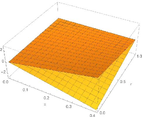
Fig. 1. Equation (20) 10th-order HPM solution at 𝑥 = 0.4, 𝑡 = 0.6, and

0 ≤ 𝑟 ≤ 1

IAENG International Journal of Applied Mathematics, 49:1, IJAM_49_1_04

(4)

[image:4.595.110.547.40.432.2] [image:4.595.294.549.50.699.2]

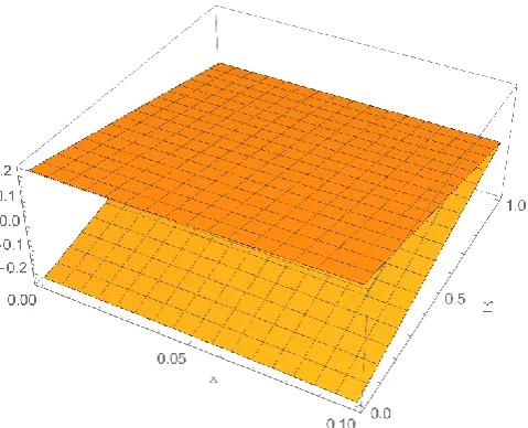
Fig. 2. 10th-order HPM solution of (20) with lower bound accuracy at 𝑡 = 0.6, 0 ≤ 𝑥 ≤ 0.4, and 0 ≤ 𝑟 ≤ 1

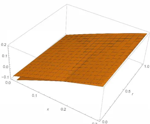
Fig. 3. 10th-order HPM solution of (20) with upper bound accuracy at 𝑡 = 0.6, 0 ≤ 𝑥 ≤ 0.4, and 0 ≤ 𝑟 ≤ 1

Fig. 4. 10-order HPM solution of (20) at 𝑡 = 0.6, 0 ≤ 𝑥 ≤ 0.4, and 0 ≤ 𝑟 ≤ 1

From tables I, II and Fig. 1 to 3 one can conclude that the 10-order HPM solution of (20) satisfies the convex triangular fuzzy number properties [24,27] for the values of 0 ≤ t ≤ 1 and 0 ≤ r ≤ 1.

Case 2. Consider the nonlinear Cauchy FRDE, where 𝑥 > 0, 𝑡 > 0,

𝜕𝑢̃(𝑡,𝑥) 𝜕𝑡 =

𝜕2𝑢̃(𝑡,𝑥)

𝜕𝑥2 + 𝑢̃(𝑡, 𝑥)(1 − 𝑢̃(𝑡, 𝑥)) (26)

𝑢̃(0, 𝑥) = [𝑟 − 1,1 − 𝑟]𝑥2_.

The initial approximation of (26) are specified by

{𝑈0(𝑡, 𝑥; 𝑟) = (𝑟 − 1)𝑥

2

𝑈0(𝑡, 𝑥; 𝑟) = (1 − 𝑟)𝑥2

(27)

According to HPM section IV we have

{

𝑈1(𝑥, 𝑡; 𝑟) = ∫ [

𝜕2𝑈0(𝑡,𝑥;𝑟)

𝜕𝑥2 + 𝑈0(𝑡, 𝑥; 𝑟)

−𝑈0(𝑡, 𝑥; 𝑟)2

]

𝑡

0

𝑈2(𝑥, 𝑡; 𝑟) = ∫ [

𝜕2𝑈1(𝑡,𝑥;𝑟)

𝜕𝑥2 + 𝑈1(𝑡, 𝑥; 𝑟)

−2𝑈1(𝑡, 𝑥; 𝑟)𝑈0(𝑡, 𝑥; 𝑟)

]

𝑡

0 (28)

. .

𝑈𝑘(𝑥, 𝑡; 𝑟) = ∫ [

𝜕2𝑈_𝑘−1(𝑡,𝑥;𝑟)

𝜕𝑥2 + 𝑈𝑘−1(𝑡, 𝑥; 𝑟)

− ∑𝑛−1𝑘−1=0𝑈𝑘−1(𝑡, 𝑥; 𝑟)𝑈𝑛−𝑘−2(𝑡, 𝑥; 𝑟)

]

𝑡 0

{

𝑈1(𝑥, 𝑡; 𝑟) = ∫ [

𝜕2𝑈0(𝑡,𝑥;𝑟)

𝜕𝑥2 + 𝑈0(𝑡, 𝑥; 𝑟)

−𝑈0(𝑡, 𝑥; 𝑟)2

]

𝑡

0

𝑈2(𝑥, 𝑡; 𝑟) = ∫ [

𝜕2𝑈1(𝑡,𝑥;𝑟)

𝜕𝑥2 + 𝑈1(𝑡, 𝑥; 𝑟)

−2𝑈1(𝑡, 𝑥; 𝑟)𝑈0(𝑡, 𝑥; 𝑟)

]

𝑡

0 (29)

. .

𝑈𝑘(𝑥, 𝑡; 𝑟) = ∫ [

𝜕2𝑈𝑘−1(𝑡,𝑥;𝑟)

𝜕𝑥2 + 𝑈𝑘−1(𝑡, 𝑥; 𝑟)

− ∑𝑛−1𝑘−1=0𝑈𝑘−1(𝑡, 𝑥; 𝑟)𝑈𝑛−𝑘−2(𝑡, 𝑥; 𝑟)

]

𝑡 0

Since the exact solution cannot be found from (26) [28], we define the residual error [29,30] to analyze the accuracy of the approximate solution approximate-analytical such that

𝐸̃(𝑥, 𝑡; 𝑟) = = |𝜕𝑈̃𝑘(𝑡,𝑥;𝑟)

𝜕𝑡 −

𝜕2𝑈̃_𝑘(𝑡,𝑥;𝑟)

𝜕𝑥2 −𝑈̃𝑘(𝑡, 𝑥; 𝑟) + [𝑈̃𝑘(𝑡, 𝑥; 𝑟)] 2

| (30) TABLEIII

EQUATION (20)15TH

-ORDER HPM OF (26) WITH LOWER SOLUTION FOR 0 ≤

𝑟 ≤ 1,𝑥 = 0.1, AND 𝑡 = 0.1

r 𝑼 HPM 𝑬

0 −0.2411520 6.514161121629058 × 10−8

0.2 −0.1914090 1.077814432148827 × 10−8

0.4 −0.1424460 1.084306144871760 × 10−9

0.6 −0.0942395 4.46025438805000 × 10−11

0.8 −0.0467649 2.20198859146592 × 10−13

1 −7.56609 × 10−19 _{1.11093988383018 × 10}−19

TABLEIV

15TH-ORDER HPM OF (26) WITH LOWER SOLUTION FOR 0 ≤ 𝑟 ≤ 1,𝑥 = 0.1,

AND 𝑡 = 0.1

r 𝑼 HPM 𝑬

0 0.22388700 2.686822725417315 × 10−8

0.2 0.18037200 4.694926836190660 × 10−9

0.4 0.13624300 4.738556769190438 × 10−10

0.6 0.09148440 1.726832565829283 × 10−11

0.8 −0.0467649 4.450606549966096 × 10−14

1 −7.56609 × 10−16 _{1.110939883830187 × 10}−19

IAENG International Journal of Applied Mathematics, 49:1, IJAM_49_1_04

[image:4.595.299.550.167.427.2] [image:4.595.47.290.468.669.2]

(5)

Fig. 5. 15th_{-order HPM solution of (26) at}_{0 ≤ 𝑟 ≤ 1}_,_{𝑡 = 0.1}_{, and}_{𝑥 =}

0.1

Fig. 6. 15th_{-order HPM solution of (26) with Lower bound accuracy}

∀ 𝑡, 𝑥 ∈ [0,0.1] and 𝑟 = 0.4

Fig. 7. 15th_{-order HPM solution of (26) with Upper bound accuracy}

[image:5.595.309.549.48.242.2]

∀ 𝑡, 𝑥 ∈ [0,0.1] and 𝑟 = 0.4

Fig. 8. 15th_{-order HPM solution of (26) at}_{0 ≤ 𝑟 ≤ 1}_,_{𝑥 ∈ [0,0.1]}_and_{𝑡 =}

0.1.

from Tables III, IV and Fig. 5 to 8 one can conclude that the 15-order HPM solution of (26) satisfies the convex triangular fuzzy number [24,27] for the values of 0 ≤ r ≤ 1. Case 3. Consider the nonlinear nonhomogeneous Cauchy FRDE, where 𝑥 ≥ 0, 𝑡 ≥ 0, 𝛼̃ = [0.9 + 0.1𝑟, 1.1 − 0.1𝑟]

𝜕𝑢̃(𝑡,𝑥) 𝜕𝑡 =

𝜕2𝑢̃(𝑡,𝑥)

𝜕𝑥2 − [𝑢̃(𝑡, 𝑥)]

2_{+ 𝛼̃𝑥}2_𝑡2 ₍₃₁₎

𝑢̃(0, 𝑥) = 0, 𝜕

𝜕𝑥𝑢̃(0, 𝑥) = 𝛼̃𝑥,

The initial approximation of (31) are specified by

{𝑈0(𝑡, 𝑥; 𝑟) = (0.9 + 0.1𝑟)𝑥 𝑈0(𝑡, 𝑥; 𝑟) = (1.1 − 0.1𝑟)𝑥

(32)

According to HPM section 4 we have

{

𝑈1(𝑥, 𝑡; 𝑟) = ∫ [

𝜕2𝑈0(𝑡,𝑥;𝑟)

𝜕𝑥2

−𝑈0(𝑡, 𝑥; 𝑟)2+ 𝛼𝑥2𝑡2

]

𝑡

0

𝑈2(𝑥, 𝑡; 𝑟) = ∫ [

𝜕2𝑈1(𝑡,𝑥;𝑟)

𝜕𝑥2

−2𝑈1(𝑡, 𝑥; 𝑟)𝑈0(𝑡, 𝑥; 𝑟)

]

𝑡

0 (33)

. .

𝑈𝑘(𝑥, 𝑡; 𝑟) = ∫ [

𝜕2_𝑈 𝑘−1(𝑡,𝑥;𝑟)

𝜕𝑥2

− ∑𝑛−1𝑘−1=0𝑈𝑘−1(𝑡, 𝑥; 𝑟)𝑈𝑛−𝑘−2(𝑡, 𝑥; 𝑟)

]

𝑡 0

{

𝑈1(𝑥, 𝑡; 𝑟) = ∫ [

𝜕2𝑈0(𝑡,𝑥;𝑟)

𝜕𝑥2 +

−𝑈0(𝑡, 𝑥; 𝑟)2+ 𝛼𝑥2𝑡2

]

𝑡

0

𝑈2(𝑥, 𝑡; 𝑟) = ∫ [

𝜕2_𝑈 1(𝑡,𝑥;𝑟)

𝜕𝑥2

−2𝑈1(𝑡, 𝑥; 𝑟)𝑈0(𝑡, 𝑥; 𝑟)

]

𝑡

0 (34)

. .

𝑈𝑘(𝑥, 𝑡; 𝑟) = ∫ [

𝜕2𝑈𝑘−1(𝑡,𝑥;𝑟)

𝜕𝑥2

− ∑𝑛−1𝑘−1=0𝑈𝑘−1(𝑡, 𝑥; 𝑟)𝑈𝑛−𝑘−2(𝑡, 𝑥; 𝑟)

]

𝑡 0

Since the exact solution cannot be found from (31) [28], we define the residual error as in case 2 to analyze the accuracy of the approximate solution approximate-analytical such that

IAENG International Journal of Applied Mathematics, 49:1, IJAM_49_1_04

[image:5.595.48.292.219.382.2] [image:5.595.48.289.418.587.2] [image:5.595.303.550.472.746.2]

(6)

𝐸̃(𝑥, 𝑡; 𝑟) = = |𝜕𝑈̃𝑘(𝑡,𝑥;𝑟)

𝜕𝑡 −

𝜕2_𝑈̃_𝑘(𝑡,𝑥;𝑟)

𝜕𝑥2 + [𝑈̃𝑘(𝑡, 𝑥; 𝑟)]

2

− 𝛼̃𝑥2_𝑡2_| ₍₃₅₎ TABLEV

12TH

-ORDER HPM OF (31) WITH LOWER SOLUTION FOR 0 ≤ 𝑟 ≤ 1,𝑥 = 0.3,

AND 𝑡 = 0.3

r 𝑼 HPM 𝑬

0 0.18977833277389260 0.00017066078329187884

0.2 0.19233109735968892 0.00017066078329187884

0.4 0.19481676927664257 0.00017066078329187884

0.6 0.19723547686377807 0.00017066078329187884

0.8 0.19958733383886260 0.00017066078329187884

1 0.20187243969820795 0.00017066078329187884

TABLEVI 12TH

-ORDER HPM OF (31) WITH LOWER SOLUTION FOR 0 ≤ 𝑟 ≤ 1,𝑥 = 03,

AND 𝑡 = 0.3

r 𝑼 HPM 𝑬

0 0.21229924682509757 0.0008404323866298136

0.2 0.21034686942973005 0.0008404323866298136

0.4 0.20832804156767476 0.0008404323866298136

0.6 0.20624272758025700 0.0008404323866298136

0.8 0.20409088014939222 0.0008404323866298136

[image:6.595.45.544.52.486.2]

1 0.20187243969820792 0.0008404323866298136

Fig. 9.12th_{-order HPM solution of (31) at}_{0 ≤ 𝑟 ≤ 1}_,_{𝑡 = 0.3}_{, and}_{𝑥 = 0.3}

[image:6.595.43.299.59.476.2]

Fig. 10.12th_{-order HPM solution of equation (31) with Lower bound} accuracy ∀ 𝑡, 𝑥 ∈ [0,0.3] and 𝑟 = 0.2

Fig. 11.12th_{-order HPM solution of (31) with Upper bound accuracy}

∀ 𝑡, 𝑥 ∈ [0,0.3] and 𝑟 = 0.2

Fig. 12.12th_{-order HPM solution of (31) at}_{0 ≤ 𝑟 ≤ 1}_,_{𝑥 ∈ [0,0.3]}_and_{𝑡 =}

0.3.

from Tables V, VI and Fig. 9 to 12 one can conclude that the 12th_{-order HPM solution of (31) satisfies the convex}

triangular fuzzy number [24,27] for the values of 0 ≤ r ≤ 1. VI. CONCLUSION

The main objective of this research with regard to approximate-analytical solution for the FRDE has been presented. We have achieved this aim by formulating and applying HPM befitting from fuzzy set theory properties. The solution provided by this method has useful feature of fast converging power series with the elegantly computable convergence of for the nonlinear problem without need to compare with exact solution. As far as we know, this is the earliest attempt to solve FRDE with HPM. Three test cases shows that the HPM is a capable and accurate method for obtaining approximate-analytical solution of FPDEs. In addition, the acquired solution demonstrates that HPM results are satisfying the properties of triangular shape fuzzy numbers.

IAENG International Journal of Applied Mathematics, 49:1, IJAM_49_1_04

[image:6.595.305.549.245.446.2] [image:6.595.48.288.504.664.2]

(7)

REFERENCES

[1] X. Guo, D. Shang and X. Lu, “Fuzzy Approximate Solutions of Second-Order Fuzzy Linear Boundary Value Problems,” Journal of Boundary Value Problems, vol. 2013, pp. 1-17, 2013.

[2] D. Qiu, C. Lu and C. Mu,” Convergence of Successive Approximations for Fuzzy Differential Equations in The Quotient Space of Fuzzy Numbers,” IAENG International Journal of Applied Mathematics, vol. 46, no. 4, pp. 512-517, 2016.

[3] H. Zhou and M. Liu,” Analysis of a Stochastic Predator-Prey Model in Polluted Environments,” IAENG International Journal of Applied Mathematics, vol. 46, no. 4, pp. 445-456, 2016.

[4] W. Kraychang and N. Pochai,” Implicit Finite Difference Simulation of Water Pollution Control in a Connected Reservoir System,” IAENG International Journal of Applied Mathematics, vol. 46, no. 4, pp. 47-57, 2016.

[5] S. Tapaswini and S. Chakraverty, “Numerical Solution of Fuzzy Arbitrary Order Predator-Prey Equations,” Applications and Applied Mathematics, vol. 8, no. 1, pp. 647-673, 2013.

[6] A. Omer and O. Omer, “A Pray and Pretdour Model with Fuzzy Initial Values,” Hacettepe Journal of Mathematics and Statistics, vol. 41, no. 3, pp. 387-395, 2013.

[7] M. F. Abbod, D.G Von Keyserlingk, D.A Linkens and M. Mahfouf, “Survey of Utilization of Fuzzy Technology in Medicine and Healthcare,” Fuzzy sets and system, vol. 120, pp. 331-3491, 2001. [8] M. S. El Naschie, “From Experimental Quantum Optics to Quantum

Gravity Via a Fuzzy Kahler Manifold,” Chaos Solution and Fractals, vol. 25, pp. 969-977, 2005.

[9] R.A. Zboon, S.A. Altaie, “Nonlinear Dynamical Fuzzy Control Systems Design with Matching Conditions,” JNUS, vol. 8, no. 2, pp. 133-146, 2005.

[10] A. F. Jameel, N. Anakira, A. K. Alomari I. Hashim, S. Momani, “A New Approximation Method for Solving Fuzzy Heat Equations,” Journal of Computational and Theoretical Nanoscience, vol. 13, pp. 7825–7832, 2016.

[11] M. Stepnicka and R. Valasek, "Numerical solution of partial differential equations with help of fuzzy transform," in The 14th IEEE International Conference on Fuzzy Systems, 2005. FUZZ '05, Reno, NV, USA, 2005.

[12] A. F. Jameel,” Semi-analytical solution of heat equation in fuzzy environment,” International Journal of Applied Physics and Mathematics, vol. 4, pp. 371-378, 2014.

[13] T. Allahviranlo,” An analytic approximation to the solution of fuzzy heat equation by Adomian decomposition method,” Int. J. Contemp. Math. Sciences. vol.4, no. 3, pp.105 – 114, 2008.

[14] J.-H. He, “Homotopy perturbation technique,” Comput. Methods Appl. Mech. Engrg., vol. 178, no. (3-4), no. 257-262, 1999

[15] J.-H. He, “A coupling method of a homotopy technique and a perturbation technique for non-linear problems,” Internat. J. Non-Linear Mech., vol. 35, no. 1, pp. 7-43, 2000.

[16] C. Chun, H. Jafari and Y.-I. Kim, “Numerical method for the wave and non-linear diffusion equations with the homotopy perturbation method,” Comput. Math. Appl., vol. 57, no. 7, pp. 1226-1231, 2009. [17] J. Biazar, and H. Ghazvini, “Convergence of the Homotopy

Perturbation Method for Partial Differential equations,” Nonlinear Analysis, vol. 10, no. 5, pp. 2633–2640, 2009.

[18] J. Biazar, and H. Aminikhah, “Study Of Convergence Of Homotopy Perturbation Method For Systems of Partial Differential Equations,” Computers & Mathematics with Applications, vol. 58, vol. (11-12), pp. 2221–2230, 2009.

[19] P. Olver, Introduction to Partial Differential Equations, Springer International Publishing, 2014.

[20] S. S. Behzadi,” Solving Cauchy reaction-diffusion equation by using Picard method,” SpringerPlus, vol. 2, no. 1, pp. 2-6, 2013.

[21] O. S. Fard, “An Iterative Scheme for the Solution of Generalized System of Linear Fuzzy Differential Equations,” World. Appl. Sci. J., vol. 7, pp. 1597-11604, 2009.

[22] S. Salahshour, “N’th-order Fuzzy Differential Equations under Generalized Differentiability,” Journal of fuzzy set value analysis, vol. 2011, pp. 1-14, 2011.

[23] D. Dubois, H. Prade, “Towards fuzzy differential calculus, Part 3: Differentiation,” Fuzzy Sets and Systems, vol. 8, pp. 225-233, 1982. [24] S. Mansouri. S, N. Ahmady, “A Numerical Method For Solving

N’th-Order Fuzzy Differential Equation by using Characterization Theorem,” Communication in Numerical Analysis, vol. 2012, pp. 1-12, 2012.

[25] L. A. Zadeh, “Fuzzy Sets,” Information and Control, vol. 8, pp. 338-353, 1965.

[26] L. A. Zadeh, “Toward A Generalized Theory Of Uncertainty,” Information Sciences, vol. 172, no. 2, pp. 1–40, 2005.

[27] O. Kaleva, “Fuzzy Differential Equations,” Fuzzy Sets Syst, vol. 24, pp. 301-317, 1987.

[28] J. Leite, M, Cecconello, J, Leite and R.C. Bassanezi, “On Fuzzy Solutions for Diffusion Equation,” Journal of Applied Mathematics, vol. 2014, pp. 1-10, 2014.

[29] S. Liang and D. Jeffrey,” An efficient analytical approach for solving fourth order boundary value problems’” Comput. Phys. Commun, vol. 180, pp. 2034–2040, 2009.