Iterative Algorithms for Computing the Takagi
Factorization of Complex Symmetric Matrices
Xuezhong Wang, Lu Liang and Maolin Che,
Abstract—The main aim of this paper is to establish iterative algorithms for computing the Takagi factorization of complex symmetric matrices. Similar to the classical iterative algorithms of computing the eigenpairs of real symmetric matrices, we derive power-like iterations for computing the Takagi values and associated Takagi vectors of complex symmetric matrices, i.e., the power-like method, the orthogonal-like iteration and the complex symmetric QR-like iteration. We analyze the convergence of these algorithms under some mild conditions. We also investigate the Jacobi-like methods for computing the Takagi factorization of complex symmetric matrices like Jacobi’s methods for real symmetric eigenvalue problems. We illustrate our algorithms via numerical examples.
Index Terms—Complex symmetric matrix, Takagi factor-ization, Singular value decomposition, Power-like method, Orthogonal-like iteration, Complex symmetric QR-like itera-tion, Jacobi-like methods.
I. INTRODUCTION
R
ECENTLY, the study of complex symmetric matrices can be divided into three categories: solving complex symmetric linear systems (see [1], [2], [3], [4], [5], [6], [7], [8], [9], [10]), computing singular value decomposition (SVD) of complex symmetric matrices (see [11], [12], [13], [14]) and solving complex-symmetric eigenvalue problems (see [15], [16], [17], [18], [19], [20]). A complex symmetric matrix can be diagonalized by a unitary matrix, which is referred to as the Autonne-Takagi factorization, sometimes shortened by Takagifactorization. It is originally proved by Leon Autonne [21] and Teiji Takagi [22]. One advantage of Takagi factorization of a complex symmetric matrix is that it reflects the symmetry of the complex symmetric matrix and thus saves the storage and computation about half.The Takagi factorization of a complex symmetric matrix has many applications, such as the Grunsky inequalities [23], computation of the near-best uniform polynomial or rational approximation of a high degree polynomial on a disk [24], the complex independent component analysis problems [25], and nuclear magnetic resonance [26].
Unfortunately, Matlab and LAPACK [27] do not support complex symmetric structures and treat it as a general complex. To compute the SVD of a complex symmetric matrix in LAPACK, the matrix is first reduced to a bidiagonal matrix, in which the symmetric structure is lost. Similar to the computation of the SVD (see [28]), a standard algorithm for computing the Takagi factorization of a complex sym-metric matrix consists of two stages. The first stage is to
X. Wang is with the School of Mathematics and Statistics, Hexi Univer-sity, Zhangye, 734000, P. R. of China. E-mail:[email protected]. L. Liang is with the School of Energy Science and Engineering, Cen-tral South University, Changsha, 410083, P. R. of China. E-mail: [email protected].
M. Che is with the School of Economic Mathematics, Southwest Uni-versity of Finance and Economics, Chengdu, 611130, P. R. of China. E-mail:[email protected].
reduce a n×n complex symmetric matrix to a complex symmetric tridiagonal matrix, and the second stage is to compute the Takagi fctorization of the complex symmetric tridiagonal matrix from the first stage. For the first stage, Qiao, Liu and Xu [29] derive a block Lanczos method for tridiagonalizing complex symmetric matrices. There are two methods for implementing the second stage: the divide-and-conquer method [30] and a twisted factorization method [13]. As we know, these methods for computing Takagi factor-ization of complex symmetric matrices are the direct method. Bunse-Gerstner and Gragg [11] derive an iterative algorithm for computing the Takagi factorization of complex symmetric matrices. In this paper, we focus on the computation of the Takagi factorization of the complex symmetric matrices by iterative methods, analogy to the symmetric QR iteration and Jacobi’s methods for real symmetric matrices.
Throughout this paper, we use small letters x, u, v, . . .
for scalars, small bold letters x,u,v, . . . for vectors and
A, B, C, . . . for matrices. For a given integer n, denote
1 : n or [n] by the set of 1,2, . . . , n. For a given matrix
A ∈ Cm×n, we use |A|, kAk2 andkAkF for the absolute
values, the largest singular value and the Frobenius norm of A. In detailed algorithmic descriptions, we write A(i, j)
or use the Matlab [31] notation A(i : j, k : l) to denote the submatrix of A lying in rowsi through j and columns
k through l. For a given vector v ∈ Cn, diag(v) is a
n×ndiagonal matrix where its diagonal entries are the same as the entries of v. More generality, for given k matrices
Ak ∈Cnk×nk,D= diag(A
1, A2, . . . , Ak)is ak×kblock
diagonal matrix with ith diagonal block equal Ai.0m×n is
am×nzero matrix andIn is the n×nidentity matrix.
The rest of our paper is organized as follows. Section 2 introduces the Takagi factorization of complex symmetric matrices. We consider how to design iterative algorithms for computing the Takagi factorization of a complex symmetric matrix and analyze the convergence of these algorithms in Section 3. In Section 4, we illustrate our algorithms via numerical examples. We conclude our paper in Section 5.
II. PRELIMINARIES
In this section, we introduce the definition of the Takagi factorization of complex symmetric matrices and establish the relationship between the Takagi factorization and the SVD of complex symmetric matrices.
A. Takagi factorization of complex symmetric matrices
The Takagi factorization [32] of a complex symmetric matrixAcan be written as:
A=VΣV>, or
(
Avi=σivi, Avi=σivi,
(II.1)
IAENG International Journal of Applied Mathematics, 48:3, IJAM_48_3_08
whereV = (v1,v2, . . . ,vn) is a unitary matrix,V> is the
transpose ofV, andΣis a nonnegative diagonal matrix. The columns of V are called the Takagi vectors of A and the diagonal elements ofΣare its Takagi values. More general,
V is called the Takagi vector matrix ofAassociated with the Takagi value matrix Σ. SinceV> =V∗, where V and V∗
denote the complex conjugate and the complex conjugated transpose of V, respectively, the Takagi factorization is a symmetric form of the singular value decomposition (SVD); but they are different. The relationships between the Takagi vectors and left-right singular vectors are listed as follows:
(a) Ifvis a Takagi vector, then(v,v)is a pair of left-right singular vectors;
(b) A left singular vector is not necessarily a Takagi vector, Xu and Qiao [30] state an example to illustrate this case. In order to analyze power-like ierations for computing the Takagi factorization of complex symmetric matrices, it is convenient to define an invariant Takagi subspace of a complex symmetric matrix, which is generalized from a Takagi vector.
Definition II.1. An invariant Takagi subspace of a complex symmetric matrix A is a subspace X of Cn, with the property that x∈X implies that Ax∈X. We also write it asAX ⊆X, where X ={x|x∈X}.
If all the Takagi values of A satisfy σ1 ≥ · · · ≥ σp > σp+1≥ · · · ≥σn, according to Definition II.1, the subspace span{v1,v2, . . . ,vp}is called apdominant invariant Takagi
subspace of a complex symmetric matrixA, wherevi is the
Takagi vector corresponding to σi withi= 1,2, . . . , p.
Meanwhile, for a given complex symmetric matrix A ∈
Cn×n, if the Takagi factorization of A is A=VΣV>, for
any unitary diagonal matrixD∈Cn×nwithdii = exp(ιϕi),
then
A= (V D−1/2)D1/2ΣD1/2(V D−1/2)> = (V D−1/2)(DΣ)(V D−1/2)> = (V D−1/2)(DΣ)(V D−1/2)>,
where ϕi ∈ (−π, π] for all i = 1,2, . . . , n. Here, DΣ and ΣD are complex diagonal matrices and the absolute values of DΣandΣD are the same as Σ.
III. ALGORITHMS
In this section, we derive four algorithms for computing the Takagi values and associated Takagi vectors of complex symmetric matrices and analyze the convergence of the algorithms. In details, we propose the power-like method of the Takagi factorization for complex symmetric matrices, this method can compute the largest Takagi value and associated Takagi vector of complex symmetric matrices; secondly, we extend the power-like method to compute a p dominant invariant Takagi subspace of a complex symmetric matrix with p > 1; we also get a complex symmetric QR-like iteration for computing the Takagi factorization of complex symmetric matrices, similar to the symmetric QR algorithm (see, e.g., [33, Chapter 5.3]) for real symmetric matrices. Under some wild conditions, we show that present three algorithms are effectiveness. Finally, Jacobi-like methods are presented to compute the Takagi factorization of complex symmetric matrices.
For the Takagi factorization of complex symmetric matri-ces, we have the following lemma.
Lemma III.1. ([34, Lemma 2]) For given two complex symmetric matricesA, B ∈Cn×n. Suppose that the Takagi factorization of A is A=VΣV>. If there exists a unitary matrix Q ∈ Cn×n such that B =Q∗AQ, then the Takagi values ofAandB are the same and the Takagi factorization ofB isB= (Q∗V)Σ(Q∗V)>.
Proof: Since the Takagi factorization of A is A = VΣV>, where U ∈ Cn×n is unitary and Σ is a positive
semi-definite diagonal matrix, according to the assumptions, we have
B=Q∗AQ=Q∗VΣV>Q= (Q∗V)Σ(Q∗V)>.
SinceQ∗Q=QQ∗=In,
(Q∗V)(Q∗V)∗=V∗(QQ∗)V =In
andB= (Q∗V)Σ(Q∗V)> is the Takagi factorization of B. We complete the proof.
The following lemma should be noted that the Takagi fac-torization of complex symmetric matrices can be determined via its singular value decomposition of matrixA.
Lemma III.2. ([11, Theorem 2.1]) Let A = UΣV∗ be singular value decomposition of the complex symmetric matrix A ∈ Cn×n with the singular values of A satisfies
σµ(1) > σµ(2) > · · · > σµ(k) and ρ(l) the multiplicity of
the singular value σµ(l), so that
k
P
l=1
ρ(l) = n. Let Ul and
Vl be the n×ρ(l) sub-matrices of U and V containing
singular vectors corresponding to σµ(l). ThenWl =Ul>Vl
is a ρ(l)×ρ(l) symmetric unitary matrix if σµ(l) > 0. If for all l ∈ [k], Wl = QlQ>l is an symmetric SVD
of Wl and D is the unitary block diagonal matrix with D = diag(Q1, Q2, . . . , Qk) thenA = (U D)Σ(U D)> is a
Takagi factorization ofA.
A. Power-like methods
Given a complex symmetric matrix A with σ1 > σ2 ≥
· · · ≥σn, let v1 be the Takagi vector corresponding to σ1,
then, we have
B= (I−v1v∗1)A(I−v1v>1) = (I−v1v∗1)A(I−v1v∗1)>
is also complex symmetric matrix and
B = (I−v1v∗1)A(I−v1v∗1)>
= (I−v1v∗1)VΣV>(I−v1v1∗)>
= VΣBV>,
whereV is the same matrix in (II.1) and
ΣB= diag(0, σ2, σ3, . . . , σn).
It is obvious that Takagi values ofB are same as those of
Aexcept forσ1. Now, we design the power-like method for
computing the Takagi pair(σ1,v1) of A. The algorithm is
summarized as Algorithm III-A. Here, we select
kAxk−λkxkk2
k|A||xk|+|λk||xk|k2
< tol
IAENG International Journal of Applied Mathematics, 48:3, IJAM_48_3_08
or
Avek−eσkevk 2
|A||evk|+|eσk||vek| 2
< tol, (III.1)
as the convergence criterion of Algorithm III-A, wheretol(> 0) is arbitrarily small.
Algorithm III.1Power-like method for complex symmetric matrices
Input: Given a complex symmetric matrixA with σ1 >
σ2≥ · · · ≥σn
Output: the Takagi valueσ1 and the Takagi vectorv1
Given an initial vectorx0∈Cn withkx0k2= 1 fork= 0,1,2, . . . do
yk+1=Axk
xk+1=yk+1/kyk+1k2
λk+1=x∗k+1Axk+1
Setσek+1=|λk+1|andevk+1= exp
ιarg(λk+1)
2
xk+1 end for
We first apply this algorithm to the case of A is a diagonal matrix with A = diag(σ1, σ2, . . . , σn) satisfies σ1 > σ2 ≥ · · · ≥ σn ≥0. In this case the Takagi vectors
are the column vectors ei (i = 1,2, . . . , n) of the identity
matrix. According to the results about the power method for diagonalizable matrices, the convergence of Algorithm III-A is easy to prove.
We prove the convergence of Algorithm III-A if A ia a diagonal positive semi-definite matrices. To analyze a more general case, we rewrite A as A = VΣV>, where V is a unitary matrix andΣ = diag(σ1, σ2, . . . , σn)is nonnegative.
Let V = (v1,v2, . . . ,vn), where the columns vi are the
Takagi vectors satisfy kvik2 = 1. Since A = VΣV∗, for
k= 0,1,2, . . ., it is easy to check that
(AA)k = (VΣV>VΣV∗)(VΣV>VΣV∗)
. . .(VΣV>VΣV∗) =VΣ2kV∗,
(AA)kA = (VΣV>VΣV∗)(VΣV>VΣV∗)
. . .(VΣV>VΣV∗)VΣV> =VΣ2k+1V>,
which follows from V>V and V∗V are the identity matrix
In.
For the case of(AA)k, let us write
x0=V(V∗x0)≡V[ξ1, ξ2, . . . , ξn]>.
It finally leads to
(AA)kx0= (VΣ2kV∗)V
ξ1 ξ2 .. . ξn =V
ξ1σ21k
ξ2σ22k
.. .
ξnσn2k
=ξ1σ21kV
1 ξ2σ22k ξ1σ21k
.. .
ξnσ2nk ξ1σ2k
.
As before, the vector in brackets converges to e1, so
(AA)kx
0 gets closer and closer to a multiple ofVe1=v1,
the Takagi vector corresponding toσ1.
Meanwhile, for the case of(AA)kA, denotes
x0=V(V>x0)≡V([ξ1, ξ2, . . . , ξn]>).
It leads
(AA)kAx0= (VΣ2k+1V>)V
ξ1 ξ2 .. . ξn =V
ξ1σ12k+1
ξ2σ22k+1
.. .
ξnσn2k+1
=ξ1σ12k+1V
1 ξ2σ22k+1 ξ1σ21k+1
.. .
ξnσn2k+1 ξ1σ21k+1
.
Similarly, the vector in brackets converges to e1, so
(AA)kAx
0 approximates closer and closer to a multiple
of Ve1 = v1, the Takagi vector corresponding to σ1.
Combining these two cases, we prove the convergence of Algorithm III-A, if the Takagi values of complex symmetric matrices satisfyσ1> σ2≥ · · · ≥σn.
It is well known that the core computation of Algorithm III-A is complex matrix-vector multiplication [28, Problem 4.2.1]. LetA=B+ιCandz=x+ιy, whereB, C ∈Rn×n
are two symmetric matrices andx,y∈Rn, then
Az= (B+ιC)(x+ιy) = (Bx−Cy) +ι(By+Cx).
Then, in each step, we need to implement Algorithm 1.2.3 in [28] eight times. Hence, the computation complexity of Algorithm III-A isO(n2)flops, whenA∈
Cn×nis complex
symmetric.
B. Orthogonal-like iteration
Our next improvement is to present a algorithm which can converge to a p(> 1)-dimensional invariant Takagi subspace, rather than one Takagi vector at each time. It is called orthogonal-like iteration (and sometimes Takagi subspace iteration or Simultaneous Iteration). This algorithm is summarized in Algorithm III-B.
We select
X
i6=j
|Λk(i, j)|2< tol, (III.2)
as the convergence criterion of Algorithm III-B, wheretol(> 0)is arbitrarily small and Λk(i, j)is the (i, j)-entry of Λk.
Here is a detail analysis of this algorithm. Assume that
σp > σp+1. If p= 1, then this method and its analysis are
identical to the power-like method. Whenp >1, we deduce
that span{Xk+1} = span{Yk+1} = span{AXk+1}, so we
have
span{X2k}= span
(AA)kX0 = span
VΣ2kV∗X0 ,
span{X2k+1}= span(AA)kAX0
= span
VΣ2k+1V>X0 .
IAENG International Journal of Applied Mathematics, 48:3, IJAM_48_3_08
Algorithm III.2Orthogonal-like iteration for complex sym-metric matrices
Input: Given a complex symmetric matrixA with σ1 ≥
· · · ≥σp> σp+1≥ · · · ≥σn
Output:Σp∈Rp×p is a nonnegative diagonal matrix and
Vp∈Cn×p such thatAVp=VpΣp andVp∗Vp=Ip
Given an initial matrixX0∈Cn×p withX0∗X0=Ip
fork= 0,1,2, . . . do
Yk+1=AXk
FactorYk+1=Xk+1Rk+1 (QR decomposition)
Λk+1=Xk∗+1AXk+1
Set Σek+1 = |Λk+1| and Vek+1 = Xk+1Dk+1,
where Dk+1 ∈ Cp×p is diagonal and Dk+1,jj = expιarg(x
∗
k+1,jAxk+1,j)
2
with j ∈ [p] and Xk+1 =
(xk+1,1,xk+1,2, . . . ,xk+1,p).
end for
Note that
VΣ2kV∗X0=Vdiag(σ12k, σ 2k
2 , . . . , σ 2k n )V
∗X 0
=σ2pkVdiag((σ1 σp
)2k, . . . ,1. . . ,(σn σp
)2k)V∗X0,
VΣ2k+1V>X0=Vdiag(σ12k+1, σ 2k+1 2 , . . . , σ
2k+1
n )V
>X 0
=σp2k+1Vdiag(( σ1
σp
)2k+1, . . . ,1. . . ,(σn σp
)2k+1)V>X0.
Since σi
σp ≥1 ifi≤p, and σi
σp <1 if i > p, we denote
diag(σ1 σp
)2k, . . . ,1. . . ,(σn σp
)2k)V∗X0=
P2k Q2k
,
diag((σ1 σp
)2k+1, . . . ,1. . . ,(σn σp
)2k+1)V>X0=
P2k+1
Q2k+1
,
where Qk(∈ C(n−p)×p) approaches zero like (σp+1/σp)k,
andPk(∈Cp×p)does not approach zero. Indeed, ifP0 has
full rank, then Pk will have full rank too. Let the Takagi
vectors matrix be V = (v1,v2, . . . ,vn) ≡ (Vp,Vbp), i.e., Vp= (v1,v2, . . . ,vp),Vbp= (vp+1,vp+2, . . . ,vn). Then
VΣ2kV∗X0=σp2kV
P2k Q2k
=σp2k(VpP2k+VbpQ2k), VΣ2k+1V>X0=σp2k+1V
P2k+1
Q2k+1
=σp2k+1(VpP2k+1+VbpQ2k+1).
Thusspan{Xk} converges to
span{X2k}= span
(AA)kX0 = span{VpX2k
+VbpY2k
o
⇒span{VpX2k}= span{Vp},
span{X2k+1}= span(AA)kAX0 = span{VpX2k+1
+VbpY2k+1
o
⇒span{VpX2k+1}= span{Vp}.
Hence, the invariant Takagi subspace spanned by the firstp
Takagi vectors, as desired.
It is well known that the core computation of Algorithm III-B is complex matrix-matrix multiplication and computing thethinQR decomposition [28, Theorem 5.2.3] ofYk+1. Let
A=B+ιC andZ =X+ιY whereB, C ∈Rn×nare two
symmetric matrices andX, Y ∈Rn×p, then
AZ = (B+ιC)(X+ιY) = (BX−CY) +ι(BY +CX).
Then, in each step, we need to implement Algorithm 1.2.3 in [28] 8p times. Hence, the computation complexity of Algorithm III-A isO(pn2)flops, if A∈
Cn×n is complex
symmetric.
Thus, we can letp=n and|X0|=In in the
orthogonal-like iteration (Algorithm III-B). The next theorem shows that under certain assumptions, we can use orthogonal-like iteration to compute the Takagi factorization of complex symmetric matrices.
Theorem III.1. Suppose that A is a complex symmetric matrix. Running orthogonal-like iteration (Algorithm III-B) on matrixAwithp=nand|X0|=In. If the Takagi values
of A have distinct values and the principal submatrices
V(1 : j,1 : j) have full rank, then Ai = Xi∗AXi
converges to DΣ, where D ∈ Cn×n satisfies |D| = In,
i.e., Aei = Vei∗AVei converges to Σ. The Takagi values will
appear in decreasing order.
Proof: The assumption about nonsingularity of V(1 : j,1 :j) for all j implies that X0 is nonsingular. Note that
Xk is a square unitary matrix, so the Takagi values of A
andAk =Xk∗AXk are the same. WriteXk = (X1k, X2k),
whereX1k haspcolumns andX2k hasn−pcolumns, thus
Ak=Xk∗AXk=
X1∗kAX1k X1∗kAX2k X2∗kAX1k X2∗kAX2k
.
Since span{X1k} converges to an invariant Takagi
sub-space ofA, span{AX1k} converges to the same subspace, X2∗kAX1k and (X1∗kAX2k)> = X2∗kAX1k converge to X2∗kX1k=0(n−p)×p. Since this is true for allp < n, every
off-diagonal entry ofAk converges to zero, soAk converges
to a complex diagonal matrix.
C. Complex symmetric QR-like iteration
Now, our goal is to attain a complex symmetric QR-like iteration for computing the Takagi factorization of complex symmetric matrices, which is needed in the proof of Theorem III.1. Algorithm III-C can realize this process.
Algorithm III.3QR-like algorithm for computing the Takagi factorization of complex symmetric matrices
Input:Given a complex symmetric matrix A0 andU0←
In
Output: Λ ∈ Cn×n is a complex diagonal matrix and U ∈Cn×n such thatAU =UΛandU∗U =I
n
fork= 0,1,2, . . . do
FactorAk =QkRk (the QR decomposition)
ComputeAk+1 ←RkQk andUk+1←UkQk
end for
In practice, the matricesXk+1in Algorithm III-B and the
matricesQk in Algorithm III-C do not need to be computed
explicitly. Here, we choose
X
i6=j
|Ak,ij|2< tol (III.3)
as the convergence criterion of Algorithm III-C, where
tol(>0) is arbitrarily small andAk(i, j)is the(i, j)-entry
ofAk withi, j∈[n]. We note that the absolute value ofAk
converges to Σ, i.e., DAkD → Σ and and UkD → V as
IAENG International Journal of Applied Mathematics, 48:3, IJAM_48_3_08
k→ ∞, where theith entry ofD isexpιarg(ai)
2
andai
is the ith entry of Ak withi∈[n].
SinceAk+1=RkQk =Qk∗AkQk,Ak+1 andAk have the
same Takagi values. We claim that theAk computed by
QR-like iteration is identical to the matrix Xk∗AXk implicitly
computed by orthogonal-like iteration.
Lemma III.3. Suppose thatA∈Cn×nis complex symmetric matrix andAk=Xk∗AXk, whereXk is the matrix computed
from orthogonal-like iteration (Algorithm III-B), then Ak
converges toDΣif all the Takagi values are different, where
D ∈ Cn×n is diagonal with |D| = In. The choice of D
depends on all matricesXk and A.
Proof: We use induction. Assume that Ak =Xk∗AXk.
From Algorithm III-C, we can derive AXk =Xk+1Rk+1,
where Xk+1 is unitary and Rk+1 is upper triangular. Then
Xk∗AXk = Xk∗(Xk+1Rk+1) is the product of an unitary
matrix Q =Xk∗Xk+1 and an upper triangular matrix R =
Rk+1 = Xk∗+1AXk; this must be the QR decomposition Ak = QR, since the QR decomposition is unique (except
for possibly multiplying each column ofQand row ofRby
−1). Then
X∗
k+1AXk+1 = (Xk∗+1AXk)(Xk>Xk+1)
= Rk+1(Xk>Xk+1)
= RQ.
This is precisely how the QR iteration maps Ak to Ak+1,
Xk∗+1AXk+1=Ak+1 as desired.
It is well known that we can use the symmetric QR iteration (for example, see [33, Chapter 5.3]) to find all eigenvalues and the eigenvectors of a real symmetric matrix. The symmetric QR iteration can be divided into two phases: 1. Given a real symmetric matrixA, find an orthogonalQ
such thatQAQ>=T is tridiagonal.
2. Employing the symmetric QR iteration to matrix T
and getting a tridiagonal matrices sequence T = T0, T1, T2, . . ., which converges to a diagonal form.
It is obvious that QR iteration keeps all theTkare tridiagonal
matrices, sinceQAQ> is symmetric and upper Hessenberg, it must also be lower Hessenberg, i.e., tridiagonal.
Similar to this process, we consider how to efficiently implement Algorithm III-C for computing the Takagi factor-ization of complex symmetric matrices. The desired process is also divided into three phases:
1. Given a complex symmetric matrix A, find an unitary
Q such that Q∗AQ = T is tridiagonal and complex symmetric, for instance, Qiao, Liu and Xu [29] derive an algorithm for implementing this purpose.
2. Apply the complex symmetric QR-like iteration to T
to get a sequence T = T0, T1, T2, . . . of tridiagonal
matrices converging to a complex diagonal form Σb.
(Note that: Bunse-Gerstner and Gragg [11] derive a unitary matrixQ by computing the QR decomposition ofT∗T to implementT converging to a diagonal form;
however, we derive a unitary matrix Q by computing the QR decomposition ofT.)
3. Convert the final complex diagonal form Σb derived
above to a positive semi-definite diagonal form Σand derive the Takagi matrixV.
We can see that QR-like iteration keeps all theTktridiagonal
and complex symmetric, sinceQ∗AQis complex symmetric
and upper Hessenberg, it must also be lower Hessenberg, i.e., tridiagonal. This keeps each QR iteration very cheap.
However, how to describe QR iteration with a shift for computing the Takagi factorization of complex symmetric matrices remains open.
D. Jacobi-like method
Jacobi’s method1 is historically the oldest method for the
eigenvalue problem, dating to 1846. For a real symmetric matrix A, Jacobi’s method does not start by reducing A
to a tridiagonal form as the symmetric QR method or divide-conquer method, instead of working on the original dense matrix. Now, we generate a Jacobi-like method for computing the Takagi factorization of complex symmetric matrices.
Given a complex symmetric matrix A = A0 ∈ Cn×n.
Jacobi’s like method produces a unitary matrices sequences
A1, A2, . . ., which eventually converges to a diagonal matrix
determined by the Takagi values.Ai+1 is obtained fromAi
by the formulaAi+1=Ji>AiJi, whereJiis a unitary matrix.
Thus
Am=Jm>−1Am−1Jm−1=Jm>−1Jm>−2Am−2Jm−2Jm−1=
· · ·=Jm>−1Jm>−2. . . J0>A0J0. . . Jm−2Jm−1≡J>AJ,
whereJ =J0. . . Jm−2Jm−1 is a unitary matrix.
If we choose each Ji appropriately, then Am approaches
a diagonal matrix Λ for large m. Thus we can write Λ ≈ J>AJ orJΛJ∗= (J)Λ(J)> ≈A. Therefore, according to (II.1) and Lemma III.1, the columns of J¯are approximate Takagi vectors ofA.
We makeJ>AJnearly diagonal by iteratively choosingJi
to make one pair of off-diagonal entries ofAi+1=Ji>AiJi.
To do this, we first consider how to find a unitary matrixQ
for computing the Takagi factorization of a 2×2 complex symmetric matrixA.
It is obvious that a2×2unitary matrixQcan be written
as
ceιϕ1 seιϕ2 −se−ιϕ3 ceιϕ4
, where
c s
−s c
is an orthogonal
matrix andϕ1+ϕ3=ϕ2−ϕ4±πwithϕi∈(−π, π], (i= 1,2,3,4). For a given 2×2 complex symmetric matrixA, we can derive a2×2unitary matrixQsuch thatQ>AQis a diagonal form by Algorithm III-C or some methods given in [11], [30], [13]. Without loss of generality, we assume that
candsare nonnegative.
We derive a Jacobi-like method for computing the Takagi factorization of complex symmetric matrices, summarized in Algorithm III-D.
Now, we analyze the convergence of Algorithm III-D and give the convergent criterion. We first define the quantity
off(A)[28, Secion 8.5.1] as
off(A) =
v u u u t
n
X
i=1
n
X
j=1
j6=i
|aij|2.
We see that off(A) is also the Frobenius norm of the off-diagonal elements. The idea behind Jacobi’s-like method is to systematically reduceoff(A). The basic step in a Jacobi-like Takagi value procedure involves these three phases:
1Demmel [33] describes some results about Jacobi’s method.
IAENG International Journal of Applied Mathematics, 48:3, IJAM_48_3_08
Algorithm III.4 Jacobi-like method for computing the Tak-agi factorization of complex symmetric matrices
Input:Given a complex symmetric matrixAandU ←In
Output:A unitary matrixU ∈Cn×n such thatU>AU is
a diagonal form
U ←In
fork= 0,1,2, . . . do
Step 1: Choose(p, q)such that|apq|= max
i6=j |aij|with p < q
Step 2: WriteAb=
app apq aqp aqq
Step 3: Compute a unitary matrixQ such thatQ>AQb
is a diagonal form
Step 4: FormJ such thatJ ←In except for
Jpp Jpq Jqp Jqq
←Q
Step 5: ComputeA←J>AJ andU ←U J
end for
(i) Choose an index pair(p, q)that satisfies1≤p < q≤n; (ii) Compute a 6-tuple(c, s, ϕ1, ϕ2, ϕ3, ϕ4)such that
ceιϕ1 seιϕ2 −se−ιϕ3 ceιϕ4
>
app apq aqp aqq
ceιϕ1 seιϕ2 −se−ιϕ3 ceιϕ4
(III.4) is a diagonal form;
(iii) OverwriteAwithB =J>AJ whereJ =In except for
(Jpp, Jpq, Jqp, Jqq) = (ceιϕ1, seιϕ2,−se−ιϕ3, ceιϕ4).
Observe that the matrixBagrees withAexcept in rows and columnspand q. Moreover, for a given matrixA∈Cn×n,
when P, Q ∈ Cn×n are unitary, the Frobenius norm of A
andP AQare the same, see, e.g., [28, Secion 2.3.5]. Hence, we find that
|app|2+|aqq|2+ 2|apq|2 = |bpp|2+|bqq|2+ 2|bpq|2 = |bpp|2+|bqq|2.
It follows that
off(B)2=kBk2
F− n
X
i=1
|bii|2=kAk2F− n
X
i=1
|aii|2
+ (|bpp|2+|bqq|2− |app|2− |aqq|2)
=off(A)2−2|apq|2.
(III.5)
In this sense, A moves closer to diagonal form with each Jacobi-like step. Since apq is the largest off-diagonal entry
in each Jacobi-like step of Algorithm III-D, then
off(A)2≤N(|apq|2+|aqp|2)
whereN =n(n2−1). It follows from (III.5) that
off(B)2≤
1− 1
N
off(A)2.
By induction, ifA(k)denotes the matrix afterkJacobi-like
updates, then
off(A(k))2≤
1− 1
N
k
off(A(0))2=
1− 1
N
k
off(A)2.
It implies that the classical Jacobi-like procedure converges with a linear rate.
Next, we consider how to improve the Jacobi-like method for computing the Takagi factorization of complex symmetric matrices. First of all, we state that the trouble of Algorithm III-D is that the updates involveO(n) complex flops while the search for the optimal(p, q)isO(n2). We can overcome
this trouble by row-by-row fashion, (see [28, Section 8.5.4]). The row Jacobi-like method for complex symmetric matrices is summarized in Algorithm 3.5.
Algorithm III.5Row Jacobi-like method for computing the Takagi factorization of complex symmetric matrices
Input:Given a complex symmetric matrixAandU ←In
Output:A unitary matrixU ∈Cn×n such thatU>AU is
a diagonal form
fork= 0,1,2, . . . do
forp= 1 :n−1 do
forq=p+ 1 :n do
Step 1:WriteAb=
app apq aqp aqq
Step 2: Compute a unitary matrix Q such that
Q>AQb is a diagonal form
Step 3:FormJ such that J ←In except for
Jpp Jpq Jqp Jqq
←Q
Step 5:ComputeA←J>AJ andU ←U J
end for end for end for
When Algorithm III-D or 3.5 is terminated, we need to convert the final diagonal form toΣand the unitary matrixU
to the Takagi vector matrixV. LetΛ = diag(λ1, λ2, . . . , λn)
the final diagonal form, the strategy is: (i) Form a diagonal matrixD as
diag
exp
ιargλ1 2
,exp
ιargλ1 2
, . . . ,exp
ιargλ1 2
;
(ii) ComputeΣandV as
Σ =|Λ|, V =U D.
When Algorithm III-C is terminated, we also need to convert the final diagonal form to the Takagi value matrixΣandU
to the Takagi vector matrixV by the above strategy. In following, for a given2×2 complex symmetric matrix
A, we consider how to more efficiently compute a unitary
Q such that Q>AQ is a diagonal form, similar to the process about computing the Schur decomposition of2×2
real symmetric matrices, (see [28, Section 8.5.2]), that is, implementing Step 2 in Algorithm III-D or 3.5.
Let the2×2 complex symmetric matrixAas
A=
a1 a2
a2 a3
=
r1eιθ1 r2eιθ2
r2eιθ2 r3eιθ3
, (III.6)
whereai∈C, nonnegativeri∈Randθi∈(−π, π]withi=
1,2,3. When the matrix
app apq aqp aqq
in (III.4) is replaced
byA, given in (III.6), and there exists a2×2unitary matrix
Q such thatB =Q>AQ is a diagonal matrix, then b12 =
IAENG International Journal of Applied Mathematics, 48:3, IJAM_48_3_08
b21= 0, that is,
b12=a1ceιϕ1seιϕ2+a2ceιϕ1ceιϕ4−a2seιϕ2se−ιϕ3
−a3ceιϕ4se−ιϕ3
=r1cseι(θ1+ϕ1+ϕ2)+r2c2eι(θ2+ϕ1+ϕ4)
−r2s2eι(θ2+ϕ2−ϕ3)−r3cseι(θ3+ϕ4−ϕ3)
= 0,
wherecandsare nonnegative, andϕ1+ϕ3=ϕ2−ϕ4±π
withϕi ∈(−π, π] andi = 1,2,3,4. We can find a unitary
matrix Q ∈ C2×2 such that Q>AQ is a diagonal form
through the process:
(i) Compute two nonnegative scalarsc andssuch that
c s
−s c
|AA|
c s
−s c
>
is a nonnegative diagonal matrix;
(ii) Choose a pair(ϕ1, ϕ2, ϕ3, ϕ4)such that
r1cseι(θ1+ϕ1+ϕ2)+r2c2eι(θ2+ϕ1+ϕ4)−r2s2eι(θ2+ϕ2−ϕ3)
−r3cseι(θ3+ϕ4−ϕ3)= 0
where ϕ1+ϕ3 = ϕ2−ϕ4±π with ϕi ∈ (−π, π] and i= 1,2,3,4.
IV. NUMERICAL EXAMPLES
In this section, the computations are implemented in Matlab Version 2013a on a laptop with Intel Core i5-4200M CPU (2.50GHz) and 7.89GB RAM. We test the accuracy and efficiency of our algorithms by computing the Taka-gi factorization or the TakaTaka-gi-like factorization of random complex symmetric matrices. Suppose that the computational accuracytolis10e−10. All floating point numbers in each example have 4 significant digits after the decimal point.
We assume that the dimension of testing matrices in each example is 100 and program our Algorithms III-A, III-B and III-C in Matlab for random generated complex symmetric matrices. Random complex symmetric matrices with pre-determined singular values in the following examples were generated as follows 2. First, a vector s, which includes n
Takagi values, is initialized. Then, a random unitary matrix
V was generated by the QR decomposition of a randomn×n
complex matrix. Finally, a complex symmetric matrixAwas obtained by the productVΣV>, where Σ = diag(s).
Example IV.1. In this example, we use Algorithm III-A
to compute the largest Takagi value and associated Takagi vector of a random complex symmetric matrixA, where the largest Takagi value of Ais larger than others ofAand its termination condition is given in (III.2).
Letσbe the largest Takagi value ofAandvbe the Takagi vector corresponding toσ. Meanwhile, denotingvb andσbas the computed Takagi vector and Takagi value, respectively, we compute the error, determined by the computed Takagi value, via
γσ=kσ−σkb 2,
and the orthogonality of the computed Takagi vectorbvmade by
γo=kbv
∗
b
v−1k2.
2Xu and Qiao [13] use a similar strategy to generate random complex symmetric tridiagonal matrices.
Fig. 1. All results about computing the largest Takagi value and associated Takagi vector of random complex symmetric matrices by Algorithm III-A
Running Algorithm III-A 200 times, Figure 1 show the computational results.
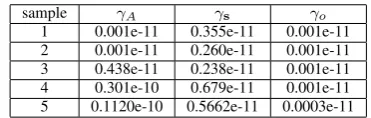
Example IV.2. In this example, we use Algorithm III-B to compute the first p Takagi values and associated Takagi vectors of a random generated complex symmetric matrixA, where the firstpTakagi values of A are larger than others ofAand the termination condition of algorithm is given in
(III.2).
Letspbe the vector determined by the firstpTakagi values
of A andVp be the Takagi vector matrix corresponding to
sp. Meanwhile, denoting Vbp andbsp as the computed Takagi
vector matrix and the vector of the computedpTakagi values, respectively, we compute the error in thepdominant Takagi factorization measured by
γA=
AVbp−Vbpdiag(bsp) 2,
the error in the computed Takagi values had by
γs =ksp−bspk2,
and the orthogonality of the computed Takagi vector Vbp
determined by
γo=
Vb
∗
pVbp−Ip
2,
where the order of all entries insp is the same as the order
of all entries inbsp.
Running Algorithm III-B 5 times, Table I show computa-tional results withp= 5.
TABLE I
ALL RESULTS ABOUT THE ERROR IN THE LARGEST5COMPUTED
TAKAGI VALUES AND ASSOCIATEDTAKAGI VECTORS OF RANDOM COMPLEX SYMMETRIC MATRICES.
sample γA γs γo
1 0.001e-11 0.355e-11 0.001e-11 2 0.001e-11 0.260e-11 0.001e-11 3 0.438e-11 0.238e-11 0.001e-11 4 0.301e-10 0.679e-11 0.001e-11 5 0.1120e-10 0.5662e-11 0.0003e-11
Example IV.3. In this example, we use Algorithm III-C
to compute the Takagi factorization of a random complex
IAENG International Journal of Applied Mathematics, 48:3, IJAM_48_3_08
[image:7.595.332.518.685.744.2]symmetric matrixA, where all Takagi values ofAare distinct and its termination condition is given in (III.3).
Let sbe the vector of all the Takagi values of A and V
be the Takagi vector matrix corresponding tos. Meanwhile, denotingVb andbsas the computed Takagi vector matrix and
the vector of the computed Takagi values, respectively, we compute the error in the Takagi factorization measured by
γA=
AVb −Vbdiag(bs) 2,
the error in the computed Takagi values made by
γs=ks−bsk2,
and the orthogonality of the computed Takagi vector Vb
characterized by
γo=
Vb
∗
b
V −In
2,
where the order of all entries in sp is the same as the order
of all entries inbsp.
Table II shows that the computed Takagi values and Takagi vectors are accurate.
TABLE II
THETAKAGI FACTORIZATION OF FIVE TESTING MATRICES WITH DISTINCTTAKAGI VALUES.
sample γA γs γo
1 0.366e-10 0.356e-10 0.001e-11 2 0.971e-11 0.263e-11 0.002e-11 3 0.437e-11 0.238e-11 0.001e-11 4 0.301e-10 0.067e-10 0.001e-11 5 0.112e-10 0.056e-10 0.003e-11
Example IV.4. In this example, the testing matrix is chosen from[3], [8]. The testing matrixAis
A= (−ω2M +K) +ι(ωC
V +CH),
where M and K are the inertia and stiffness matrices, respectively; CV and CH are the viscous and hysteretic
damping matrices, respectively; andωis the driving circular frequency.
We take CH = µK with µ = 0.02 being a
damp-ing coefficient, ω = 2π, CV = 12M, and K the five
point centered difference matrix approximating the negative Laplacian operator with homogeneous Dirichlet boundary condition on a uniform mrsh in the unit square[0,1]×[0,1]
with the mesh size h = m1+1. In this case, the matrix
K ∈Rm×m possesses the formK =Im⊗Vm+Vm⊗Im
withVm=h−2tridiag(−1,2,−1)∈Rm×m.
In our example, we assume that m = 3. The meanings of γA, γs and γo are given in Example IV.3. For different
matricesM, all results are given in Table III.
TABLE III
γA,γsANDγoFOR COMPLEX SYMMETRIC MATRICES.
M In 2In 5In 10In 15In
γA 0.114e-11 0.114e-11 0.025e-10 0.468e-11 0.083e-10 γs 0.049e-11 0.186e-11 0.112e-10 0.712e-11 0.122e-10 γo 0.001e-11 0.002e-11 0.001e-10 0.001e-11 0.002e-11
TABLE IV
γA,γsANDγoFOR COMPLEX SYMMETRIC MATRICES.
σ2 5 10 50 80 100
γA 0.157e-10 0.235e-11 0.311e-11 0.236e-11 0.146e-11 γs 0.371e-10 0.294e-11 0.112e-11 0.209e-11 0.219e-11 γo 0.001e-10 0.001e-11 0.001e-11 0.001e-11 0.001e-11
Example IV.5. In this example, the testing complex symmet-ric matrix is chosen from [4], [6]. The testing matrix A is given in
A=H+σ1In+ισ2In,
In addition, we setσ1= 100andHis the same as the matrix
K given in Example IV.4. We see that A is the coefficient matrix of the complex symmetric linear system leaded by the following form of the Helmholtz equation:
−4u+σ1u+ισ2u=f,
where σ1 and σ2 are real coefficient functions, u satisfies Dirichlet boundary conditions in[0,1]×[0,1].
In our example, we assume that n = 9. The meanings of γA, γs and γo are given in Example IV.3. For different
positive scalarsσ2, all results are given in Table IV.
V. CONCLUSIONS
In this paper, we derive iterative algorithms for computing the Takagi factorization of complex symmetric matrices and analyze the convergence of these methods. Numerical exam-ples show that our algorithms are accuracy for implementing this process.
However, we do not consider how to implement efficiently these algorithms for computing the Takagi factorization, if the Takagi values are not always distinct. In the near future, we shall consider how to improve these algorithms for computing the US-eigenpairs of a complex symmetric tensor and the U-eigenpairs of a generic complex tensor, which is referred to Ni, Qi and Bai [35] or the generalized tensor eigenvalue problems [36], [37], [38].
ACKNOWLEDGMENT
The author would like to thank the editor and referees for their detailed comments which greatly improved the presentation of the paper.
REFERENCES
[1] S. R. Arridge, H. Egger, and M. Schlottbom, “Preconditioning of complex symmetric linear systems with applications in optical tomography,”Appl. Numer. Math., vol. 74, pp. 35–48, 2013. [Online]. Available: http://dx.doi.org/10.1016/j.apnum.2013.06.008
[2] O. Axelsson and A. Kucherov, “Real valued iterative methods for solving complex symmetric linear systems,” Numer. Linear Algebra Appl., vol. 7, no. 4, pp. 197–218, 2000. [Online]. Available: http://dx.doi.org/10.1002/1099-1506(200005)7:4¡197::AID-NLA194¿3.0.CO;2-S
[3] Z.-Z. Bai, M. Benzi, and F. Chen, “On preconditioned MHSS iteration methods for complex symmetric linear systems,” Numer. Algorithms, vol. 56, no. 2, pp. 297–317, 2011. [Online]. Available: http://dx.doi.org/10.1007/s11075-010-9441-6
[4] D. Bertaccini, “Efficient preconditioning for sequences of parametric complex symmetric linear systems,” Electron. Trans. Numer. Anal., vol. 18, pp. 49–64 (electronic), 2004.
[5] V. E. Howle and S. A. Vavasis, “An iterative method for solving complex-symmetric systems arising in electrical power modeling,”
SIAM J. Matrix Anal. Appl., vol. 26, no. 4, pp. 1150–1178, 2005. [Online]. Available: http://dx.doi.org/10.1137/S0895479800370871
IAENG International Journal of Applied Mathematics, 48:3, IJAM_48_3_08
[6] C.-X. Li and S.-L. Wu, “A double-parameter GPMHSS method for a class of complex symmetric linear systems from Helmholtz equation,”
Math. Probl. Eng., pp. Art. ID 894 242, 7, 2014. [Online]. Available: http://dx.doi.org/10.1155/2014/894242
[7] T. Sogabe and S.-L. Zhang, “A COCR method for solving complex symmetric linear systems,” J. Comput. Appl. Math., vol. 199, no. 2, pp. 297–303, 2007. [Online]. Available: http://dx.doi.org/10.1016/j.cam.2005.07.032
[8] S.-L. Wu, “Several variants of the Hermitian and skew-Hermitian splitting method for a class of complex symmetric linear systems,”
Numer. Linear Algebra Appl., vol. 22, no. 2, pp. 338–356, 2015. [Online]. Available: http://dx.doi.org/10.1002/nla.1952
[9] X. Wang and Z. Wang, “Preconditioned parallel multisplitting usaor methods for h-matrices linear systems,”IAENG International Journal of Applied Mathematics, vol. 44, no. 1, pp. 45–52, 2014.
[10] M. U. Rehman, C. Vuik, and G. Segal, “Preconditioners for the steady incompressible navier-stokes problem,”IAENG International Journal of Applied Mathematics, vol. 38, no. 4, pp. 223–232, 2008. [11] A. Bunse-Gerstner and W. B. Gragg, “Singular value decompositions
of complex symmetric matrices,” J. Comput. Appl. Math., vol. 21, no. 1, pp. 41–54, 1988. [Online]. Available: http://dx.doi.org/10.1016/0377-0427(88)90386-X
[12] M. Ferranti, T. H. Le, and R. Vandebril, “A comparison between the complex symmetric based and classical computation of the singular value decomposition of normal matrices,” Numer. Algorithms, vol. 67, no. 1, pp. 109–120, 2014. [Online]. Available: http://dx.doi.org/10.1007/s11075-013-9777-9
[13] W. Xu and S. Qiao, “A twisted factorization method for symmetric svd of a complex symmetric tridiagonal matrix,”Numer. Linear Algebra Appl., vol. 16, no. 10, pp. 801–815, 2009.
[14] J. B. Erway, R. F. Marcia, and J. A. Tyson, “Generalized diagonal piv-oting methods for tridiagonal systems without interchanges,”IAENG International Journal of Applied Mathematics, vol. 40, no. 4, pp. 269– 275, 2010.
[15] S. S. Ahmad and V. Mehrmann, “Perturbation analysis for complex symmetric, skew symmetric, even and odd matrix polynomials,” Elec-tron. Trans. Numer. Anal., vol. 38, pp. 275–302, 2011.
[16] P. Arbenz and O. Chinellato, “On solving complex-symmetric eigenvalue problems arising in the design of axisymmetric VCSEL devices,” Appl. Numer. Math., vol. 58, no. 4, pp. 381–394, 2008. [Online]. Available: http://dx.doi.org/10.1016/j.apnum.2007.01.019 [17] P. Arbenz and M. E. Hochstenbach, “A Jacobi-Davidson method
for solving complex symmetric eigenvalue problems,”SIAM J. Sci. Comput., vol. 25, no. 5, pp. 1655–1673 (electronic), 2004. [Online]. Available: http://dx.doi.org/10.1137/S1064827502410992
[18] J. Danciger, “A min-max theorem for complex symmetric matrices,”
Linear Algebra Appl., vol. 412, no. 1, pp. 22–29, 2006. [Online]. Available: http://dx.doi.org/10.1016/j.laa.2005.06.020
[19] V. I. Hasanov, “An iterative method for solving the spectral problem of complex symmetric matrices,” Comput. Math. Appl., vol. 47, no. 4-5, pp. 529–540, 2004. [Online]. Available: http://dx.doi.org/10.1016/S0898-1221(04)90043-0
[20] Q. Zhang and X. Wang, “Complex-valued neural network for hermitian matrices,”Engineering Letters, vol. 25, no. 3, pp. 312–320, 2017. [21] L. Autonne,Sur les matrices hypohermitiennes et sur les matrices
unitaires. Rey, 1915, vol. 38.
[22] T. Takagi, “On an algebraic problem reluted to an analytic theorem of carath´eodory and fej´er and on an allied theorem of landau,” in
Japanese Journal of Mathematics: transactions and abstracts, vol. 1, no. 0. The Mathematical Society of Japan, 1924, pp. 83–93. [23] C. Pommerenke, Univalent functions. Vandenhoeck & Ruprecht,
G¨ottingen, 1975, with a chapter on quadratic differentials by Gerd Jensen, Studia Mathematica/Mathematische Lehrb¨ucher, Band XXV. [24] L. N. Trefethen, “Near-circularity of the curve in complex Chebyshev
approximation,”J. Approx. Theory, vol. 31, no. 4, pp. 344–367, 1981. [Online]. Available: http://dx.doi.org/10.1016/0021-9045(81)90102-7 [25] P. Comon, “Independent component analysis, a new concept?”Signal
processing, vol. 36, no. 3, pp. 287–314, 1994.
[26] A. D. Bain, “Chemical exchange in NMR,” Progress in Nuclear Magnetic Resonance Spectroscopy, vol. 43, no. 3, pp. 63–103, 2003. [27] E. Anderson, Z. Bai, C. Bischof, S. Blackford, J. Demmel, J. Dongarra, J. Du Croz, A. Greenbaum, S. Hammerling, A. McKenney et al.,
LAPACK Users’ Guide. SIAM, 1999, vol. 9.
[28] G. H. Golub and C. F. Van Loan,Matrix Computations, 4th ed., ser. Johns Hopkins Studies in the Mathematical Sciences. Johns Hopkins University Press, Baltimore, MD, 2013.
[29] S. Qiao, G. Liu, and W. Xu, “Block Lanczos tridiagonalization of com-plex symmetric matrices,” inOptics & Photonics 2005. International Society for Optics and Photonics, 2005, pp. 591 010–591 010.
[30] W. Xu and S. Qiao, “A divide-and-conquer method for the Takagi factorization,”SIAM J. Matrix Anal. Appl., vol. 30, no. 1, pp. 142–153, 2008. [Online]. Available: http://dx.doi.org/10.1137/050624558 [31] I. T. M. Works,Matlab Reference Guide. Math Works, Incorporated,
1992.
[32] R. A. Horn and C. R. Johnson,Matrix Analysis, 2nd ed. Cambridge University Press, Cambridge, 2012.
[33] J. W. Demmel, Applied Numerical Linear Algebra. Society for Industrial and Applied Mathematics (SIAM), Philadelphia, PA, 1997. [Online]. Available: http://dx.doi.org/10.1137/1.9781611971446 [34] R. C. Thompson, “Singular values and diagonal elements of complex
symmetric matrices,”Linear Algebra Appl., vol. 26, pp. 65–106, 1979. [Online]. Available: http://dx.doi.org/10.1016/0024-3795(79)90173-3 [35] G. Ni, L. Qi, and M. Bai, “Geometric measure of entanglement and
U-eigenvalues of tensors,”SIAM J. Matrix Anal. Appl., vol. 35, no. 1, pp. 73–87, 2014. [Online]. Available: http://dx.doi.org/10.1137/120892891 [36] C. Cui, Y. Dai, and J. Nie, “All real eigenvalues of symmetric tensors,”
SIAM Journal on Matrix Analysis and Applications, vol. 35, no. 4, pp. 1582–1601, 2014.
[37] W. Ding and Y. Wei, “Generalized tensor eigenvalue problems,”SIAM Journal on Matrix Analysis and Applications, pp. 11–36, 2015. [38] T. G. Kolda and J. R. Mayo, “An adaptive shifted power method for
computing generalized tensor eigenpairs,” SIAM Journal on Matrix Analysis and Applications, vol. 35, no. 4, pp. 1563–1581, 2014.