Steady Capillary Gravity Waves on Deep Water

WAVES ON DEEP WATER

Thesis by

Benito Miguel Chen Charpentier

In Partial Fulfillment of the Requirements for the Degree of

Doctor of Philosophy

California Institute of Technology Pasadena, California

1979

ACKNOWLEDGEMENTS

I like to thank my adviser, Professor Philip G. Saffman, for suggesting the topic of this thesis and for his invaluable help and patience during its development. I would also like to express my gratitude to the faculty, fellow students and staff of the Applied Mathematics department for many useful suggestions and for these interesting years.

My stay at Caltech was possible thanks to support by the Consejo Nacional de Ciencia y Tecnolog1a, Mexico, and to a Graduate Research Assist antship. I am indebted to Control Data Corporation for providing me with time on their STAR 100 computer, without which the calculation:· would not have been possible.

A~STRACT

The properties of capillary-gravity waves of permanent form on deep water are studied. Two different formulations to the problem are given. The theory of simple bifurcation is reviewed. For small amplitude waves a formal perturba-tion series is used. The Wilton ripple phenomenon is re-examined and shown to be associated with a bifurcation in which a wave of permanent form can double its period. It is shown further that Wilton's ripples are a special case of a more general phenomenon in which bifurcation into subharmonics and factorial higher harmonics can occur.

Numerical procedures for the calculation of waves of finite amplitude are developed. Bifurcation and limit lines are calculated. Pure and combination waves are continued to maximum amplitude. It is found that the height is limited

in all cases by the surface enclosing one or more bubbles. Results for the shape of gravity waves are obtained by solving an integra-differential equation. It is found that the family of solutions giving the waveheight or equivalent parameter has bifurcation points. Two bifurcation points

CHAPTER

1.

2.

3·

TABLE OF CONTENTS

Acknowledgements Abstract

Table of Contents INTRODUCTION

FORMULATION OF THE PROBLEM

1.1 The Fourier Series Expansion 1.2 The Vortex Sheet Formulation 1.3 Some Integral Properties 1.4 Simple Bifurcation

WEAKLY NON-LINEAR WAVES

2.1 Pure and Combination Waves 2.2 Wilton Ripples

2. 3 Wilton Ripples as a 2 _.1 Bifurcation

PAGE i i i i i iv 1

8 8 14 18 22

27 27 33 39

2.4 Combination (N,M) Waves 42

2.5 The M-+N and N-+M Bifurcations, N

>

!M 46 2. 6 The Case 1 < N

<

iM 48

2.7 The Case N=1, M~4 49

2.8 Bifurcation of (1,3) Combination Waves 52

NUMERICAL PROCEDURES

3.1 The Fourier Series Method 3.2 The Vortex Sheet Method

CHAPTER

4.

5·

3.3 Arclength Continuation

FINITE AMPLITUDE CAPILLARY-GRAVITY WAVES 4.1 Introduction

4. 2 The Finite Amplitude 2-+1 and 2-+ 3 Bifurcations

4.3 The Finite Amplitude M .. N Bifurcation

PAGE 66

72 72

74

with N

>

t

79

4.4 The 1-+M Limit Line 81

4.5 Waves of Maximum Height on Deep Water 83

FINITE AMPLITUDE GRAVITY WAVES 5.1 Introduction

5.2 Numerical Results for Regular Waves

89 89

of Class 1 95

5.3 Bifurcation of Regular Class 2 Waves:

a New Type of Symmetrical Solution 98 5.4 Bifurcation of Regular Class 3 Waves 102

5.5

Discussion 106

APPENDIX A APPENDIX B FIGURES TABLES REFERENCES

108 110 112

INTRODUCTION

Since the last century, there has been an undecaying interest in the study of periodic, irrotational, permanent surface waves on a deep heavy inviscid fluid. Most of the work done considers gravity as the only restoring force. In his now classic paper of 184?, Stokes (27) proposed the existence of a solution for the non-linear problem as a perturbation series in the amplitude. He calculated the first three terms of the series and found that the speed of propagation

c

depends on the amplitude. When he revised this paper in 1880 (28), he found i t simpler to reformulate the problem using the complex potential as the independent variable. He also added an appendix proving that if the surface has a cusp, the internal angle is 120°. Since, as the amplitude grows, the crests become steeper and the troughs shallower, he speculated that the highest wave would have a 120° corner and a wide shallow trough. Michel l

(1?) and Yamada

(32)

incorporated this singular behavior into the approximate calculation of waves of maximum

solutions for waves of any height up to almost the maximum. His surface profiles tend to those of Michell and Yamada, as the waveheight increases. Longuet-Higgins (13), using the same method as Schwartz, found that the wavespeed and the energy are not monotonic functions of the waveheight, and established some integral and differential properties of gravity waves. Longuet-Higgins and Fox (15) constructed asymptotic expansions close to the 120G-cusped wave of greatest height and showed that both the wavespeed and the energy oscillate infinitely often as the limiting wave is approached, and moreover, the maximum slope is greater than 30°. The stability of finite amplitude, steady gravity waves to infinitesimal sinusoidal disturbances has also been investigated by Longuet-Higgins (14). He determined

that for a superharmonic perturbation (the wavelength of the perturbation is less than that of the unperturbed steady wave) there is an instability at

h!J ..

:=·

0.13'1

which is also the value for which the wavespeed has a max-imum. When the perturbations are subharmonic, he found that for small amplitudes all modes are neutrally stable; become unstable when the waveheight reaches a certain value corresponding to the Benjamin

& Feir (1) instability, and,

as the amplitude continues to increase, become stable and then unstable again at about h/,.\:::0.129

force, Crapper (4) solved the problem analytically. He

found that the wavespeed decreases monotonically with the

waveheight, and that the highest wave encloses a bubble.

For higher amplitudes the surface crosses itself making

the solution unphysical.

Harrison

(6)

approximated the solution to the problem

with both surface tension and gravity by a Fourier series

using Stokes' hypothesis that the nth Fourier coefficient

is nth order in the amplitude. He calculated three terms

and found that the approximation broke down when the

wave-length was such that the wavespeed was the same as the

speed of waves with a half or a third of the wavelength.

He showed that the profiles for waves of very short and

very long wavelength are essentially different. Wilton

(3

1

)

extended the expansion to fifth order and showed how to

correct the inconsistency at the critical wavelengths

~

AN:4n(NT/pg)

,

where

N

is an integer greater than 1,

I

the surface tension,~ the density of the fluid and

3

the

acceleration due to gravity. He proposed that at the

crit-ical wavelengths, the first and Nth harmonics are of the

same order and all the others of smaller order. He found

~

further that two different solutions exist at A

1

·~n(4~,)

,

the so-called Wilton ripples.

Pierson and Fife (21) using the method of strained

coordinates extended Wilton's solutions to wavelengths

second order expansion valid near _.\

3 ( ).. 3 =2.

99

om in water)

using the technique of multiple scales and found three

different profiles.

Schooley (22) observed experimentally in wind generated

waves profiles close to those predicted by Wilton near

A=2.44 em. However, McGoldrick (16) using a wavemaker

could not produce a uniform profile for

A

=2.

44

em. The

physical existence of capillary-gravity waves near the

critical wavelengths is still an open question.

Results about the mathematical existence and

unique-ness are few and most are limited to small amplitude. For

gravity waves \\=0), Nekrasov (20) formulated the problem,

for symmetric waves about verticals through the crest and

trough, as a non-linear integral equation. He proposed a

series solution and proved the convergence for sufficiently

small amplitude, but did not give the radius of convergence.

Levi-Civita (12) used a similar series to prove the

exis-tence of water waves for sufficiently small amplitude. His

proof yields solutions that are symmetric with respect to

crest and trough, but, contrary to popular belief, he did

not prove that all gravity waves must be symmetric. More

recently, Krasovskii

(9)

gave an existence proof valid for

waves of finite amplitude with slopes measured from the

horizontal less than )0°. Keady and Norbury

(7)

reformulated

the problem using the inverse of the speed at the crest

series for all crest speeds down to but not including zero. The highest wave with an stagnation point at the crest is the only wave not included in the proof, which allows even

0

for the existence of waves with slopes greater than

30

.

Garabedian

(5)

using variational methods gave another existence proof and, under the assumption that there is only one crest and trough per period, proved that the waves are symmetric about the crest and trough. A corollary of his proof is the uniqueness of symmetric waves with the same crests and troughs. He could not prove symmetry for waves whose crests or troughs have unequal heights. Toland

(30)

proved the existence of the highest wave having a stagnation point at the crest, and showed that the crest has to be either a 120° cusp or the limit point of a sequence of steep ripples.

For capillary-gravity waves, Sekerzh-Zen'kovich (24) gave the outline of an existence proof. Zeidler

(33)

did a comprehensive study of existence and uniqueness proofs, together with the functional analysis methods used. One of the most important results is his constructive proof of existence and uniqueness for capillary-gravity waves of sufficiently small amplitude for all wavelengths, except the critical ones found by Wilton. He supposed symmetry of the waves.

for sufficiently small amplitude and it is likely that

they cease to exist when the amplitude reaches some finite

critical value. Gravity waves do not appear to exist when

VA)

o.

ILl 'l. Also, capillary waves cease to exist for

h/J...)

o. 7 )0. The limiting wave touches i tsel:f and encloses

a bubble but the shape is otherwise smooth. The results of

Wilton (31), Pierson and Fife (21) and Nayfeh (19) show

that capillary-gravity waves are not unique, even for

wave-lengths not equal to the critical ones. It is not obvious

that permanent nonsyrnmetrical capillary-gravity waves of

sufficiently large amplitude do not exist. Wilton ripples

are not symmetric with respect to all their crests or

troughs.

Our main objective is to investigate the properties

of capillary-gravity waves, analytically for small

ampli-tude and numerically for ampliampli-tudes up to the maximum. We

will study the bifurcation of waves into subharrnonics and

fractional higher harmonics, and show that finite amplitude

capillary-gravity waves are not unique. We will also give

evidence of nonuniqueness for gravity waves. We will

re-strict ourselves mainly to symmetrical waves about a crest

or a trough. But for gravity waves we will explore the

possi-uili ty of nonsyrnmetrical solutions. The mathematical

existence and stability of the solutions are beyond the

In chapter 1, the physical problem is established and

the mathematical equations derived. Some integral and

differential properties of water waves are formulated. A

review of simple bifurcation and arclength continuation is

given.

In chapter 2, we consider the form of weakly

non-linear waves of permanent shape on deep water under the

effects of both surface tension and gravity. A formal

per-turbation series is used to find uniformly valid solutions

and to establish the bifurcation of waves. Wilton ripples

are a special case of this phenomenon.

Chapter

3

is the development of the numerical

proce-dures used to solve the problem for finite amplitude.

Chapter

4

contains the numerical results for finite

amplitude capillary-gravity waves.

Chapter

5

is the numerical study of high amplitude

CHAPTER 1

FORMULATION OF THE PROBLEM

1.1 The Fourier series expansion.

We consider periodic, steady or permanent,

one-dimen-sional, inviscid, irrotational, progressive water waves of

finite amplitude on deep water otherwise at rest, under

the influence of both gravity and surface tension. The

density of the upper fluid, usually air, is neglected.

We take rectangular coordinate axes Ox'y', with Ox'

horizontal and Oy' vertically upwards in a frame of

refer-ence moving with the wave. Let 2=~~~y denote the complex

physical coordinate. We study the wave in a window of

horizontal extent

L,

where Lis an integral multiple of

the wavelength

A

,

that is defined as the shortest period

of the wave. Let c be the wave speed and

h

the height,

defined as the vertical distance between the top of the

highest crest and the bottom of the lowest trough. Denote

the components of the velocity vector in the direction Ox'

and Oy' by~ and~. respectively, the pressure by

?

and

density )' of the fluid will be taken equal to 1 with no

loss of generality.

Since in this frame of reference the motion is steady,

the equations of motion for an inviscid, incompressible

and one-dimensional fluid are

~+~-.::0

~')( ~1

u. ~..,.. .r ~ -:: _

cP..

'b'X

()6

~

u.

~

+ \]"

}.\t -=- -~ - ~

b'X ~~ d ~~ •

Further, since the motion is irrotational~

(1.1.1)

(1.1.2)

(1.1.3)

~- ~::

0 (1.1.4)

ax

(}~

and there exists a complex potential w~; +-1."{1 such that

u..- ..\ v ::

~

_d~ ( 1 1 _{• •} 5)

For incompressible fluids, we have Bernoulli's integral

(1.1.6)

where

A

is a constant.

Next consider the boundary conditions. Let f(x~~)=O

describe the surface, then the condition that there is no

transfer of matter across the surface gives the first

boundary condition

That is, the velocity at the surface is tangential to the

surface. Since the surface is not known a priori, we need

an additional condition. This is the dynamic condition

-p:

-

T

"R"

(1.1.8)

where

T

is the surface tension and R the radius of

curva-ture of the interface taken positive when the surface is

concave upwards.

Since the surface is a streamline, say

'I' •

o, i t is

more convenient to work with ~ as a function of the complex

potential. The fluid occupies the region 'f'~ 0. See figure

1. The equation of continuity (1.1.1) and the

irrotation-ality of the fluid (1.1.4) give

(1.1.9)

on 'f'~

o.

The boundary conditions imply that

f"+

1.~'1'- ~:::

cl.(t-b)

(1.1.10)

on

't'

=o. In ( 1.1.10) <:J,=

l

d~/cAwl ~'

evaluated on the surface,

Y

is the height of the free surface above some or1g1n.

Bernoulli's constant is written as c~(l-b}, where c i s the

wavespeed. The magnitude of the wave determines the

param-eter

b,

but its precise specification depends upon the

choice of origin for

Y.

For instance, i f

Y

is measured

from the mean water level, then the argument in Lamb (10,

to show that

b=O.

(See appendix A). However, we find i t convenient in our discussion to measure "'( , and the horizon-tal coordinate, from a crest or a trough (i.e. a local maximum or minimum of Y) where w is also supposed to

van-ish. In this case

b ~

1-1.. V..o c1..

+ l. T ,

R

0 c'1..

(1.1.11) where suffix ₀ refers to the origin and ~₀ is the speed at the crest or trough.

We are going to use two completely different methods to find solutions to the problem. The first one consists in expressing

z

in terms of the complex potential w by a Stokes type expansion. The second is to consider the sur-face as a vortex sheet and obtain an integra-differential equation for the problem. This method will be developed in section 1.2.

Returning to the first method, let

..0

z.: W- ~.A.

b.

<;" ("'

e.><p(-:tl\1'\.i'AikL)

+

~

C l.lT

4-

n .2.1T

(1.1.12)

which satisfies Laplace's equation (1.1.9). Since ~(0)=0,

we have that

Co

is given in terms of all the other C~ 's. The unknowns are the complex constants en, the wavespeed and the parameter

b.

They are determined by Bernoulli's equation (1.1.10) and by the amplitude of the wave.

potential

¢ .

Evaluation of ~ and ~and substitution into

(1.1.10), which must be satisfied foro~ p~cL, together

with a specification of the amplitude, provides the

neces-sary equations for the unknowns.

We now assume further that the waves are symmetrical

about the origin; that is, we suppose that a crest or a

trough exists about which the wave is symmetrical and

choose i t as the origin. It was proved by Levi-Civita (12)

and others that permanent symmetric gravity waves exist.

Zeidler (33) proved the same for capillary-gravity waves.

To our knowledge, i t has not been proved that all waves

must be symmetric. However, this is a matter for further

study and we shall restrict attention to symmetrical waves.

Then i t can be supposed that the constants Cn~An+~Bn, say,

are real (i.e. Bn~o) and the parametric equation of the

interface is

oO

X==-

_L

S

t

h "

_L

A ...

_{__..., Sirl.}

ns

2.1T lTT I I')

(1.1.13)

y

~

LlT

f._

~

((OS Y\F -1)

;l_ Y\ .J ~ (1.1.14)

where

(1.1.15)

'2_ I l .\_

and the origin is taken at

5

=o. Since g,.;c.~ (X'

t-Y

)

and

R-'

=

cx'Y"-x"Y')/(X' 2

+Y'

2)312 , where I =d/d"_5, equation

(1.1.16)

Because of the assumed symmetry, s~n is also a crest or trough and i t is sufficient to satisfy ( 1.1.16) for o~

5

~ TT •

This equation was given by Wilton (31), with a slightly different notation.

The unknowns in (1.1.16) are the An, n

=

1,2, ••• , the wave speed c, and the parameter

b.

The period L is supposed known. Therefore a fUrther condition is necessary to

spec-ify the solution. This is usually taken to be the wave-height

h,

say, i.e. vertical distance between crest and trough, or perhaps the energy of the wave measured relative to a fixed frame, or the leading coefficient

A

_{1 •} We found from experience that none of these parameters were univer-sally useful for describing the bifurcation phenomenon to be described in this work, and in fact we have been unable to construct a parameter which characterized the magnitude of the wave for all the phenomena in a satisfactory way. For the computations we used the following method of

characterizing the wave magnitude in terms of an amplitude parameter £. • The sequence A1,

Al.).

~

I

;\Y\ \

=

1. Then we take

L

AY\ An::

f. I

(1.1.17)

Different classes of waves correspond to various choices

of the sequence ~ . The parameter E. may be positive or

negative. This approach is not particularly elegant and

lacks a clear physical interpretation, but i t is the most

convenient one we have found so far. The basic difficulty

is the lack of a parameter which is a monotonic function

of a physically significant wave magnitude. An alternative

approach is to specify b as the amplitude parameter.

Our task will be to study the solutions of (1.1.16).

1.2 The vortex sheet formulation.

There are several alternative schemes which reduce

the calculation of the wave profile to the solution of

non-linear integra-differential equations. See, for

example, Nekrasov (20), Milne-Thompsen (18) and Bloor (2).

We have found convenient a method of this type based on

the fact that the surface of a water wave is a vortex

sheet.

We work in the coordinate system fixed in the wave,

see figure 1. Since the inertia of the air is neglected,

the air (or upper fluid) is identically zero. Then the

surface of the wave is a vortex sheet of strength '?t\$) ,

where s is arclength along the surface and ~ is the

tangen-tial velocity of the fluid. The surface has the parametric

representation

Zl

s)

=

X(

s}+ J....

Y

(S) . Let

u... -

A.v denote

the components of velocity in the fluid. Then from the

Biot-Savart law, the velocity at z.

=

x + ...l ~

u..-iv-

=-

i.._Joo=t(S,)

ds,

+ J..

c.

:nr z.-

2cs,)

:z

-..c

is given by

(1.2.1)

The reason for the

1c

is that the Biot-Savart law gives

the velocity only to the extent of an arbitrary constant.

The velocity induced by the vortex sheet has equal and

opposite limits as ':} .... -too. Hence, to make the velocity as

'j - + a ( ) equal to zero and the velocity as ~ _.-0 0 equal to

c, the additive constant must be

ic.

Plemelj's formula states that

llm ( f(s,)

ds, ::

Pj

f

(SJ

Js, .-;

~

n

_:f,.W_

2

-+Zfs)j

z-7As,)

Zts)-Z{s,)

2

cs>

(1.2.2)

The minus sign is for z. approaching the surface from above,

and the plus sign from below.

P

denotes the Cauchy

princi-pal value.

From (1.2.1) and (1.2.2), we have

(1.2.3)

where

8(s)

is the slope of the surface measured from the

d.Z

~e

g

_

-i.e

cl

s

=

e

J Js -

e

"

(1.2.4)

where the overbar denotes the complex conjugate. Thus

'""'

~ ~(s)

cli ::: _

.:i..

Pj 51

<s,)

cls,

-+ -\. <-. cis l.TT -..o L(s)· 'Z(S,)

Bernoulli's equation (1.1.10) gives I

~(s)= (c~(l-b)-:z~)(S)-t-2T

)2

R<s)

(1.2.5)

(1.2.6)

Equation (1.2.5) is then a non-linear, singular, integra-differential equation for

Z(s).

It can be simplified by a change of variable. Introduce

¢

or

5

as independent

variables instead of

s.

Then

(1.2.7)

and aO

-

- _;_ Pj d¢,

+-Lc 2.1r - o D Zf~)-7

MJ

2 ~

(1.2.8)

or since the problem is periodic of period L for

Z

and

cl

for

¢ ,

using that

<><> _,

,L

c.L

p

r

d

¢,

=

L

PJ

d

rA

.::

JL

p(

<.Ot[n (7.(~)

-

Zl~,)~d¢,J

(

1. 2.

9)

~-a

71¢)-lf¢,)

~"

--

o

7A~)-

Lf¢,)-Yll L

~

L

and writing

z-

l

s

~lT ~ (1.2.10)

(1.2.11)

where

..L

=

:2..

rr

Tm (

Q

d

S

/I

c.lij

3

)

R L d ~4

J

5

d

5

•

(1.2.12)

To equation (1.2.11) must be added some condition that specifies the magnitude of the wave. The simplest procedure conceptually is to specify

h= Yl'\axlY)-mi.n(Y). (1.2.13)

Equation (1.2.11) then has solutions of period 2rr in

J ,

provided ~ is sufficiently small. These solutions are, however, not isolated for

(1.2.15)

is obviously also a solution of (1.2.11) and (1.2.13) for arbitrary values of ~ , ;(0 and

'J

₀ • Equation ( 1. 2 .15)

describes the same wave displaced horizontally and vertical ly, moving in the same or opposite direction, with the

X(O)

=

0, (1.2.16)

The three equations (1.2.16) then suffice in principle to

determine the three arbitrary constants in the general

solution (1.2.15). Implementation of (1.2.16) can be made

automatic when the solution is assumed to be symmetric.

However, for T=O we also prepared a numerical method which

does not assume that the wave is necessarily symmetric.

The purpose was twofold; first to provide a check on

cal-culations assuming symmetry, and second to try and find

nonsymmetrical solutions. Implementation of (1.2.16) then

proved difficult until overcome by a trick; see equation

(3.2.13) of chapter 3.

Equations (1.2.11) and (1.2.16) together with (1.2.13)

or an equivalent measure of wave magnitude, provide us in

principle with a complete set of equations to determine

water waves of finite amplitude. This approach is very

usefUl in calculating high amplitude gravity waves.

1.3 Some integral properties.

Integral properties of interest are the kinetic and

potential energies per unit length. The kinetic energy

K

is measured in a frame fixed relative to the fluid.

(1.3.1)

The physical and potential planes are sketched in figure 1.

The last equality of (1.3.1) is Stokes' theorem. The

inte-gration along the boundary is in the clockwise direction.

Using the periodicity of the solution, and that the fluid

is at rest at ::1 = -co , the only contribution to the line

integral is from the boundary OAB where

'f-::-

cl

₎

~

=

~-eX.

It follows that

(1.3.2)

Here

Y is the mean height defined as

L l.1T

Y=

L_

J

YJx

::_L

l

Y~

ds

(1.3.3)

o

L

o

I

Substituting (1.1.13) and (1.1.14) into (1.3.3) and

inte-grating we have

(1.3.4)

Now, using (1.1.14) and (1.3.4), the kinetic energy is

The potential energy has two contributions, V~ due to gravity and

VT

due to surface tension. The gravitational

L y 2.1T

v~

-=

~ j

j _

~

'j d'j d

x :::

.i.. ( ,

Y l_ 9 l )

~

J

5

J

o '(

.2 L

)o

cl_5 (1.3.6) and upon substitution of the parametric equations for

X

(1.3.7)

or calculating the integral,

(1.3.8) The surface tension contribution is

L

2n

~

vT=

I

((ds-dx)=

t (

l

[[&X)~(J'<}]

-ax}Js

Jo

.)0

l

d

~

J1

a)

,J (1.3.9)

or using (1.1.13) and (1.1.14)

~n ~

VT =

~ joi[(I+~A

..

~~~j)\(4A"str~V\g)L]~-IJ~_5.

(1.3.10)

Other important physical quantities are the momentum per unit length

l y

1

=

t

J

~ ~

)(

d'j d

>( )

0 --o

(1.3.11)

the excess flux of momentum due to the wave

defined by

L y

f

=

T

J

(

[

-p +

~

\

~\

L +

d (

J-

Y )]

1x

dJ

d

X •

0 - cD

(1 . .3.1.3)

Levi-Civita (11), Starr (25), Starr and Platzman (26) and Longuet-Higgins (1.3) established the following rela-tions

(1..3.14)

5

=

L!

K-3\J'~ (1 • .).15)

f

o= (

3 T -

2

v~

>

c

(1..3.16)

Of these three relations, only the first one is valid for

T

~

o .

Provided ~

f

0 , the following relation gives a useful check on the accuracy of the calculations

(1 • .).17)

We will prove i t following Lamb (10, p. 420) and Starr (25)

in appendix A.

If the amplitude is allowed to vary, the following differential relation governs the rates of change of K, V~

and c

(1..3.18)

(1 • .).18) is valid only for gravity waves. It is also a

follows Longuet-Higgins

(13)

and is given in appendix B.

1.4

Simple Bifurcation.

We can write

(1.1.16)

or

(1.2.11)

and

(1.2.16),

to-gether with some amplitude equation such as

(1.1.17)

or

(1.2.13),

abstractly as

(1.4.1)

where the element ~is the solution (the Fourier

coeffi-cients AV~'"'=1,2,

... ,

or the wave profile for 0~ _5 £-2TT

the wavespeed

c

and the parameter b), t i s the parameter

which determines the magnitude of the wave and

T

is the

surface tension. Since we are only going to consider

branches of solutions of

(1.4.1)

that have one of the two

parameters £ or T constant, the notation can be simplified

by writing

(1.4.1)

as

(1.4.2)

where ~ now represents the parameter that is allowed to

vary.

In practice,

&

and~ will be finite dimensional

vec-tors arising from the discretization of the governing

equations. To follow solution branches of

(1.4.2),

determine

branches at the latter, we follow Keller (8) and introduce the arclength S in ( u._, f') space. Instead of finding solu-tions of ( 1.

4.

2) in the form u.-= U.l'f>) with the parameter

"P

given, we calculate u-= u.ts) ,

f::.

pCS) • An additional equation of the form

(1.4.3)

is needed to determine

'P

as a function of S • A point

(u.\~o),p{s,)) on the branch is a regular point if the Fr~chet derivative &u.(u l).,),pl5o)) is non-singular. Otherwise we have a critical point. In general, a critical point is either a limit or a bifurcation point, but i t can be both. At a limit point, the value of

f

has a maximum or a minimum and ~ is not a single valued function of

-p

in the vicini-ty of the point. Since the arclength

S

is always monotonic on a branch, limit points disappear when

s

is the parame-ter. At a bifurcation point two or more solution branches intersect.

The following relations hold if

s

=5₀ is a simple bifurcation point where two smooth solutions intersect non-tangentially I

di.m

N

{

&: )

= codlWI

ft. (

&-;)

=

I }

&

o

E

R(fr.o)

1' v..

null space and

R.

the range. Denote by

¢,

(1.4.4)

if

unit norm elements which span

/V(&:)

and the adjoint space

!Vl&:~)

respectively.

(1.4.4)

implies the existence of a

unique element

¢

0 such that

-If

It follows from the definition of ~

(1.4.5)

and

(1.4.5)

that

(1.4.6)

this equation provides a way to check for bifurcation and

distinguish i t from limit point behavior.

To find the branches at a simple bifUrcation point we

first differentiate (1.4.2) twice with respect to

s

,

eval-uate at 5₀ , and multiply the second derivative on the left

by

'f.*" ,

giving for each branch ( lAs0~lJ.~<S.\, fs0~f,(5.,)):

(1.4.7)

The right hand side of

(1.4.8)

is zero because

&;

is in

the range of

&

~ and y-'₁ .>J- is orthogonal to the range of &~

Since the null space of is one dimensional, we have

from ( 1.

4. 7)

with

(1.4.10)

Substituting (1.4.9) into (1.4.8) gives the quadratic equation

A

()(., 1. t

B

o<.,o<o + (

o<o ;;

l 0 (1.4.11)

with

"1- 0

A

~

'f.

&

U.\A ~I

¢,

(1.4.12)

B

::

r,'*

{

&u: (

~

0

¢,

+

~

¢o)

t 2 {y

u;

~~}

(1.4.13)

(1.4.14)

Solution of the quadratic, the so called algebraic

bifurcation equation, gives the branches intersecting at the bifUrcation point and makes i t possible to switch from one branch to the other. Note that prior knowledge of one

branch gives one root of the quadratic. For further details

and a general treatment see Keller (8). In chapter

3

we describe the actual procedure by which solution branches were followed and simple bifurcation points found. As we shall see later, i t is likely that more complex behavior may be associated with high order bifurcation, but the

CHAPTER 2

WEAKLY NON-LINEAR WAVES

The object of this chapter is to study the solutions

of (1.1.16) and determine the slope of symmetrical waves

of permanent form. We shall examine analytically the

properties of solutions of small but not infinitesimal

magnitude as described by formal perturbation series. In

later chapters we obtain approximate solutions for finite

amplitude using numerical methods.

2.1 Pure and combination waves.

If we suppose that the magnitude of the wave is

small, we may expand equation (1.1.16) in powers of the An•

We obtain after some algebra an expression

"'0 oo ..o oa

t

)A b-

2

~n

t-/j:

L

A~

-

K

L

n

A~+

L

o(f

Af'

CO'>

p..$

I I :2 ) I

~~ ~

+

f

~

[

~r,,

c.os(

p-~))

+

f

f

)~

cos

(

p+~)

_s]

AP

A~

+

~

[

"(p-p +pff cos

1p_5]

A~

Pt'}

- oa«>

+

~

[

o(1'ff cos

1

s

+

"?f

1'f ws 3

r

3

J

A~

+

~-

~

[ o(

~

1'1' cos

~ ~

+

?

~

PP <.os ( 1p-₁₎

3

1tr

where the omitted terms are quartic and higher order, and

o(f = ~ - M. + K .()I o(

=

l..f-

-Is

K. (p+~~

I / I f>~ 2 ' >

13

::

)"-

-

t }( (

f-t

1 \

f,1

o<.fff -=

' l

+

1

J<-p J

(2.1.2)

PN'f' = -/ +

'i )(

f~ o<.'~fF ::. -2

ft+

.t

I{ (lpt

t),

~

fP

= )"

~

f

X. {2ptj) I

P;,p

~

-

3)"-

-1-

%

K {2pt1).

In these equations the dimensionless parameter

(2.1.3)

measures the relative importance of surface tension and

gravity, while

(2.1.4)

is a dimensionless form of the unknown wavespeed.

We characterize the wave magnitude in terms of an

amplitude parameter

f.

by taking

(2.1.5)

where the sequence ...\,,

A..l.,

,t ₃

'

...

is chosen depending on the

type of wave we want to study, If we now, following Wilton

( Jl), equate the coefficients of c.os ~~ in (2.1.1) to zero

for n:O,I,l, ••• , we obtain an infinite number of algebraic

correct, in the sense that truncation at order M by

setting Al'l =o for n>M and ignoring coefficients of (OS l'l~

for n

>

M gives, together with ( 2.1. 5) , Mt 1. equations for the M ~ 1. unknowns A,,A1, ... A,..,,JA J b • The problem seems,

there-fore, to be well posed, although convergence proofs are

lacking.

Let us suppose now that all the A~ are zero except

AN

,

say. Then

AN=

f._ , and i f

lc l

L..'

I ,

we can expect a

solution to exist in which the

An

are powers of E.. • In

particular, the solution will have A~= o unless VI is a

multiple of

N ,

and further

"''tv)

AYI

-= f) {c. ) (2.1.6)

when

N

divides ~ . We shall call a solution of this kind

a pure wave of degree

N

and magnitude ~ . Pure waves of

degree 1 were calculated by Wilton up to order E5 , using

the ansatz expressed by (2.1.6). A pure wave of degree

N ,

amplitude

c

and k=~' , say, consists, of course, of pure

waves of degree 1, wavelength

LfN ,

and the same magnitude

with !r:. =- N2.1<..' • It might therefore be thought that there

would be no loss of generality in following Wilton and

re-stricting attention to pure waves of degree 1, but this

actually turns out not to be the case.

Since

AN

is the dominant coefficient in a pure wave

of degree

N ,

we expect that the coefficient of

AN

in

(2.1.7)

Only the harmonics of Los NS are generated and their coef-ficients are uniquely determined by the equations derivable from (2.1.1), provided the coefficients

G'< ( _p N) := j_ - u + K f -:1 0

-f / -N (2.1.8)

for

f

a multiple of~ • Elementary algebra shows that (2.1.8) is violated for -p=-rN (i.e. o<.p(N)=o) i f

J<

=

Yf.,..N

4

) .

When (2.1.8) fails, i t is found that the ansatz (2.1.6) is inconsistent and the expansion fails.

Wilton examined in detail the case N=l '("- 2 }(; .L

' - ' 2

He showed that in this case the ansatz (2.1.6) should be replaced by the assumption that both

A,

and

A.,_

are of order

E •

It is then found that in the infinitesimal limit

(2.1.9)

wavelength L and

i

L have the same phase speed when K-=

1 .

Wilton noted that the ansatz might also fail when

, but stated that only £or Y-=2. was there any

ambiguity in the value of'

Ar

for K-= YY • This statement

is literally correct for r>3 , but as we shall see in the

course of this work there can be ambiguity for K slightly

greater than

Yr

.

It is false £or Y~3 . A difference

between ~'""= 2.. and the other cases is that only in the

former case is the important interaction quadratic. For

v- ~ 3 , the interaction is cubic.

We can generalize Wilton's approach by examining the

possibility that, with K given, c>{-p vanishes £or two or

more values o£ ~ • From the definition o£ ~~ , i t is easily

seen that a necessary and sufficient condition is

(2.1.10)

In this case, o<.~

=

o(M :::.

o ,

i£

(2.1.11)

Even though Y~ may be an integer with many decompositions

into a pair o£ factors, £or only one decomposition at a

time can o<"' and o(M vanish. These considerations suggest

the existence of combination waves, in which for an

arbi-trary pair o£ integers N and

M ,

the coefficients

AN

and

AM

are o£ comparable order t.. and all the other

An

are

expansion should fix the ratio of

Atv

to

AM

as for the

Wilton ripple which is the particular case N

=

I , M-= 2

We shall see below that combination waves exist for all

sets of positive integers M and

N

for appropriate value

of K • The Wilton ripples are the simplest but not

particu-larly typical example.

Clearly without loss of generality, we can now suppose

that M and N are copr'ime, and we take for definiteness

I~

N

L M • We will call such a wave a combination ( 1\1, M)

wave. Multiplication of

N

and

M

by an integer

corre-sponds to dividing

K

by the square of the same integer.

The concept of pure and combination waves can be

extended to finite amplitude although not without some

ambiguity. The wave will be said to be pure i f the

coeffi-cient of the lowest order harmonic clearly determines the

wave in a unique manner. Thus, Crapper's exact capillary

waves, for which in our notation

1'\

A~

=

LJ

Y\ (

A,;

_{4 )} J n

=

2) 3, '1, . .. .J (2.1.12)

are pure waves of degree 1. Similarly, Stokes gravity

waves of permanent form found by expansion in

A, ,

where

Al

=A~+

tJ (

A,

4) etc, are pure waves. If, on the other hand,

the lowest order harmonic is relatively insignificant or

does not specify the wave uniquely in a clear way, we

shall speak of a combination wave. A precise classification

as we shall see a combination wave for some value of X

may be the analytic continuation of a pure wave for a

different k. •

The existence of combination waves of small magnitude

will now be considered. First we deal with the case M~lN.

2.2

Wilton ripples.

Combination waves with N"" I , M :::. 1 are typical of

the case M:: lN • We suppose that A, and

A,_

are both B(£)

and that the remaining A~ are of smaller order. The con -sistency of the ordering is easily checked a posteriori.

Then the coefficients of cos

5

give the equations

and c.os 2)

(1-JA+K)A, +(;t- ~

K)A,Al-=

()((3)~

(J.-u+.<.K)A~+lu.-.lK)A4 _{-= 0(E.}3

)

2 / • I 2. I •

in ( 2.1 .1)

(2.2.1)

(2.2.2)

These equations, together with a form of the amplitude

equation (2.1.5)

(2.2.3)

constitute three equations for the three unknowns

A, ,

A

4 ,

p-

in terms of the given parameters /( and {_ •

solution with

A -::. o

_{I '}

A

₄

=

2.€

j

(2.2.4)

In this wave,

, A

=<'(E"'), and i t is a pure

ll'"l

wave of degree 2. There is nothing special about K.

=

f

for

this wave. (There may of course be ambiguity around J<.::: V(2:p) ,

-p>l .)

We wish to consider now the solutions :for which

A.

:1= 0 •

For X not close to

i,

there is a solution with

which is recognisable as a pure wave of degree 1. (The

difficulties that might arise when

K

~

Y

111 , ~"'~) 2 , are the

subjects of the following sections.) But this solution is

not uniformly valid as K approaches

t.

To obtain a

uni-formly valid solution, we solve

(2.2.1)

for

r

and

substi-tute into

(2.2.2),

neglecting the 0(£3) terms on the right

hand sides. This gives

Al=

_I

1-+K--fKAl

1-A._

~

( 1-2.. K )Al. + ( l+ K.)

Al

2-K.

(2.2.6)

(2.2.7)

The dependence on t. can be found by substituting into

(2.2.)),

but i t is better to work with

(2.2.7)

which

con-tains the whole phenomenon of Wilton's ripples in a simple

First we note that i f X is not close to

i,

we recover

the pure wave ( 2. 2. 5) • If 1<

=

t ,

we obtain Wilton's

for-mula (2.1.9). Equation (2.2.7) in fact contains the

uni-formly valid relation between

A,

and

A

₂ • Once the

rela-tion between A, and Al. is established to lowest order,

the equations derivable from (1.1.16) or (2.1.1) allow in

principle the unique calculation of the remaining A~ to

arbitrary order.

There are now two alternative methods of procedure.

The first is to interpret (2.2.7) as a quadratic giving

A

2

in terms of

A. •

Thus

Al.

-::

-I+ .2.K. "t

J

{(I-2 k )4+ 4 (2-K ){It K )All.}

'2.( It K.) • (2.2.8)

This is the approach of Pierson and Fife (21), who studied

the nature of Wilton ripples for K close to

i

by a

some-what different method than that used here. It appears that

one should take the positive square root for K .::

-t

and

the negative square root for K

>

1

, in order to join

smoothly with the pure wave (2.2.5) for K not close to

t.

However, this leaves uncertain the status of the other

root.

The second and more informative approach is to

inter-pret (2.2.7) as specifying

A, .

given

A

₁ • Then we see

that solutions exist only if

A,

is such that the right

hand side is positive. In figure 2.1, we have plotted the

It is convenient to use k :: K/( 1-+K.) in order to include the capillary waves in the figure. Notice that

A,

vanishes

when

Al.:: o

and

A,_

=

3

k-

1 Accessible regions are hatched.

The analysis is for weakly non-linear waves, so we cannot

say which regions are accessible when

A"l.

is 0(1) • From

Crapper' s calculations, we know that A~ '- I. 65 4 for pure

capillary waves of degree

1.

(it is equal to

1.819

for the

pure capillary wave of degree 2.) For the pure gravity

wave of degree

1,

Schwartz's

(23)

results suggest an upper

limit of about 0.18 for

A,

(or 0.29 for the limiting pure

wave of degree 2). Note that these results also suggest

that the highest wave does not have the greatest value of

A'l ,

so that the

A

2,

K

plane will be covered more than once

near the limiting wave.

The boundary of the region is unknown at present and

needs numerical work for its determination. The results of

such study will be reported in chapter

4.

There is, of

course, no reason to believe that the accessible region is

singly covered, so the topology of the covering may be

fairly complicated. The point

K

=

2.13

,

K

=

1.. , has the

property that

A,_

vanishes at this value for the weakly

non-linear pure wave of degree 1. It is an apparent

singu-larity caused by the choice of plot and does not have a

physical significance.

The point K

=

t

is a fundamental

A • _.

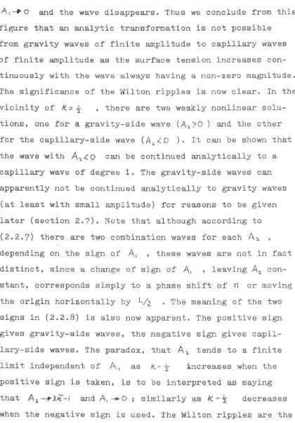
o

and the wave disappears. Thus we conclude from this

figure that an analytic transformation is not possible

from gravity waves of' finite amplitude to capillary waves

of' finite amplitude as the surface tension increases

con-tinuously with the wave always having a non- zero magnitude. The significance of' the Wilton ripples is now clear. In the

vicinity of' I(=

±

, there are two weakly nonlinear

solu-tions, one for

a

gravity-side wave (A~)O) and the other for the capillary-side wave (A

1

~0 ). It can be shown that

the wave with

Al

<

o

can be continued analytically to a

capillary wave of' degree 1. The gravity-side waves can

apparently not be continued analytically to gravity waves

(at least with small amplitude) for reasons to be given

later (section

2.7).

Note that although according to

(2.2.7)

there are two combination waves for each

A,

depending on the sign of'

A. ,

these waves are not in fact distinct, since a change of sign of'

A.

,

leaving

A2.

con-stant, corresponds simply to a phase shift of'

n

or moving

the origin horizontally by

L/2,

•

The meaning of' the two

signs in

(2.2.8)

is also now apparent. The positive sign

gives gravity-side waves, the negative sign gives capil~

lary-side waves. The paradox, that

A,

tends to a finite

limit independent of'

A.

as k..- .L

4 increases when the

positive sign is taken, is to be interpreted as saying

that

A1.

~3k-1 and

A.-

0 ; similarly as 1<.

-1:

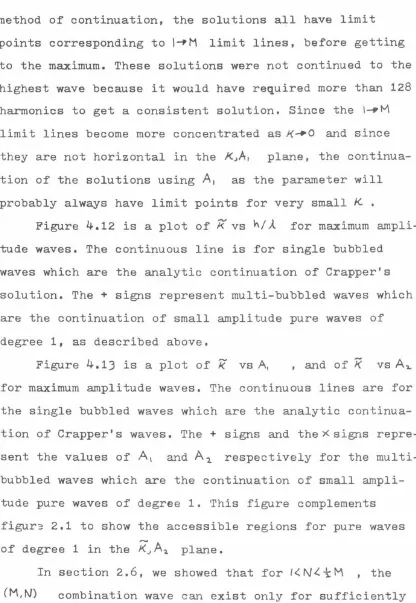
decreases [image:42.530.64.484.83.686.2]

particular solutions on the line ){ ::

1 ,

1<. =

f

, but

there are clearly neighboring solutions £or K not exactly

equal to

!.

There is an interesting di££erence between

capillary-side and gravity-capillary-side waves. For A~<.. 0 , the crests o£ the

combination waves are o£ equal height and unequal spacing,

whereas the troughs are o£ unequal depth but uni£orm

separation Lfl • The waves are symmetrical about troughs

but not about crests. The converse is true for the

grav-ity-side waves. Thus the analytic continuation o£ a pure

capillary wave o£ degree 1 into a Wilton ripple is

asso-ciated with the creation o£ another trough, or going in

the reverse direction with the disappearance o£ a trough.

Conversely the appearance or disappearance o£ the

gravity-side Wilton ripple as K._-.L

:L becomes small or large is

associated with the creation or disappearance o£ a crest.

Sample pro£iles showing these changes are shown in £igure

2.2.

We now discuss an interpretation of Wilton's ripples

as a bifUrcation phenomenon in which the wavelength o£ a

pure wave can suddenly double when i t attains a certain

2.) Wilton ripples as a 2-+1 bifurcation.

The regions marked 'no solution' in figure 2.1 show where no combination (1,2) wave exists. However, pure waves

of degree 2 exist in these regions (provided the magnitude is less than some as yet unknown value). Thus if we de-scribe waves by the relation between

A,

and

A

'l. , we see

that there are solutions with

A,:::

0 for arbitrary

A

4

(within the limits of existence of pure waves), and there are also solutions with non- zero

A

1 provided, according to ( 2. 2. 7) ,

or (2.).1)

for k <... 2 . The result ( 2. J .1) is of course limited to

I A

1

1<<.

I , and is therefore valid only for K close to

t.

These results are shown graphically in figure 2.), where we sketch

A,

vs

A"t

for fL <...

t

and K

>

-5:- , with

).k-1:1<<..\

,

as given by equation (2,2.?). For a given

value of I(

>-!:' ,

there always exists a pure wave of degree 2, marked by the

A2..

axis. For

A

2

<.o

there is also a

combination wave which is a capillary-side wave. Thus

A

1=0

combination wave of twice the wavelength. The bifUrcation

wave has the shape shown in figure 2.2, the middle crest

being slightly decreased (

A

1 ) 0 ) or increased (A ,I.. O ) ,

and is a gravity-side wave. Similarly for K <

t

,

there

is a trivial bifurcation at

A

₄

=

0 into a combination gravity-side wave, and a non-trivial bifurcation at

Al.

:::(.lk-1)/( l+K.) of the pure wave of degree 2 into a

combina-tion wave. For I(::

-I ,

the figure would reduce to the two straight lines

A, ::

.:t

A

₂ •

It is to be noted that although the solutions

A,

and

-A

1 are mathematically distinct in the formulation, they

are physically the same wave displaced a distance L/~ .

The difference between the pure wave of degree 2 with A~

and -

A

2 is a similar transformation. The reason why

bifurcation occurs for A~

>o

when k

>

y ,

say, and not also for A~<o

,

lies in the constraint that the wave is

symmetrical about the origin. When Al ) 0 , the origin is a crest and the bifurcated waves for /(

> -i

are symmetrical about crests. They are not symmetrical about troughs and

therefore bifurcation with

Al

<

0 , when the origin is a trough, is excluded for K

>

-f

It is to be expected that the bifurcation phenomenon will be associated with a change in stability of the pure

wave to small disturbances, the combination wave being

perhaps stable while the pure wave loses its stability.

although calculations of stability are straightforward

they seem to be rather tedious and we shall defer the

question for later study. The present work is restricted

to an investigation of possible forms of steady waves.

Suppose now that we have a weakly non-linear pure

wave of height h (vertical distance between crest and

trough) and wavelength

A. •

This wave can be described as a

pure wave of degree 2, with

(2.).2)

Then i f the amplitude of the wave is such that

h

>

4

A Ill

'l.T - ..L \

311 ~A 1. 4 ) (2.J.J)

the wave can bifurcate into a combination wave of

wave-length

2A.

In other words, waves such that ~~T/jAL is

close to

i

could spontaneously double their wavelength when

the amplitude exceeds the critical value given by (2.J.J).

The locus of bifurcation points given by (2.J.J) is

only valid for small amplitude. The shape of the curve for

•

finite amplitude can be investigated by numerical means, to

be described in chapter

4.

We now continue the analysis by

2. 4 Combination ( N , M ) waves.

The coefficients

A.,.,

of a permanent wave can be

de-rived in principle from the equations obtained by setting

the coefficients of cos n ~ to zero in the master equation

(2.1.1). As mentioned earlier, pure waves of degree 1 can

be constructed by solving recursively, and the series

presumably converges if A, is sufficiently small, provided

K

"*

YM • If K

=

YM , c:>(M ~ 0 and the first approximation

to

AM

gives

At1:?

.a • The previous sections studied this problem for the case M

=-

1. , and it was seen that the way

to avoid the difficulty and obtain a uniformly valid

solu-tion was to suppose that

A,

and

A

1 are both of order E •

We now study the existence of a combination (

N ,

M )

wave, with l. N 't"M , for which

A

=c;)(£)

A

=B(£.)

/{

-

-L-=~(CS")

N J H J

Ml\l

(2.4.1)

and the other coefficients of higher order. The value of s

is to be determined, and will be seen below that 5= 2 •

Without loss of generality, we suppose that

N

and

M

are coprime and I~N<M

.

The case N = \ ,

M-=

3

has special

features and is deferred to a later section.

With the assumption (2.4.1) and supposing that

N

< M ,

N

-:t

~

M

, N

1=

-J

M ,

it follows from ( 2.1 .1) that

A =B(,(·)

A

=0(t.l.)

A

::

O(C)

A

=

0CE

1

) (2.4.2)

and all remaining coefficients are of higher order.

Equat-ing in ( 2 .1.1) the coefficients of cos

Ns ,

c.o5 M ~ , cos 2~5,

c.os .ZM 5 , c.os (N-rM)s and c.os(M-N) ~ to zero, and neglecting

terms smaller than 0([3) , we obtain

-+2o(

A A

+o<

A A'

-o

M•M+t.t M M+N NMM N M - '

(2.4.3)

(2.4.4)

(2.4.5)

(2.4.6)

(2.4.7)

(2.4.8)

The~ and

p

coefficients are given by (2.1.2). However, we

can simplify the expressions by substituting the leading

order values K:: 'IMN , )A=

YM

-t

'IN ,

except in <><rv and

o<M.

p( _ _L _ _1_ .::>( _ J_ _ ...L o<.

=

_1_ o<. _ :l.N-M

.l.N - M ltV J lM- 1'1 .lM ) M-+N t-\HJ J M-tv- MlM-N)

-J -..L o< - _ L . v-.M,M+N - 4t1 ' NJ M+N - 4111 )

= J_ - j_

M lN'

1'\ - J_ j _ 1-M, N Ll M + 4

rv ,

<='<, - I I o(

NfoJN - 8M -

N

l MMI'-1

~ --_2_ I

MIVtv - I.{N -

1M

.1

It is clear £rom these equations that consistency requires

(2.4.9)

The procedure now is to substitute £rom (2.4.5),

(2.4.6), (2.4.7), (2.4.8) into (2.4.J) and (2.4.4), and

then eliminate

)A

to obtain a relation between AM and AN

(2.4.10)

where

'( =

CN+ 10M} (2.4.11)

N I?MN I

It is evident from these expressions that ~N ) 0 for

all appropriate pairs N , M , while ¥M ) 0 for N

>

f

M and

~M /.... 0 for

N

<.

tM .

Then provided AN and

AM

satisfy the

relation ( 2. 4.10) , where 2tv't M , 3N

+

M , a combination wave exists. This wave exists in addition to pure waves of

degree

M ,

for which AN= 0 • Pure waves of degree

N

also

exist if t\1)\ , and have

Ay.,=O •

If

N=-\

,

the pure wave has a more complicated structure and will be discussed

separately. If

I

K-

A-w \

>) E. 4 , the combination waves are

not infinitesimal and must be studied numerically.

Convergence of the expansions has not been proved, but

there is no reason to doubt existence i f the amplitudes are

sufficiently small and K is sufficiently close to 1_{/MN •}

The pure and combination waves all move with approximately

the same speed

c~

::

.1.1:..

(_L

-+

.J._)

2.

5

The M-+N and N-.M bifurcations, N

>

..r

M

We consider first the case that tV

>1M

and examine the implications in terms of bifurcation phenomena.

Equa-tion

(2.4.10)

is now a hyperbola in a plot of

AN

vs

AM

as shown in figure 2.4. There are two cases according as

The figure can be interpreted as follows. For

arbi-trary values of /{- '/M

rv

of (5(Et.) , there exist pure waves

of degree

N

and

M

of (;}([) amplitude. However, the pure

waves of degree M can bifurcate when

Ji

A

=

-:! [ ( _!_ - k) M-N ] for

M MN YM '

I

J( c( Mf\/ '

(2.5.1)

into a combination (N,M) wave. Similarly, the pure wave of

degree

N

can bifurcate into a combination (N)M) wave

when

for i-( )

.-l-M IV •

(2.5.2)

If K

=

YHN , the hyperbolae degenerate into two pairs

of straight lines

(2.5.3)

There are four types of combination waves depending

on the signs of

AN

and

AM •

These waves appear to be

different, they cannot be brought into coincidence by a

arbitrary (small) amplitude. The accessible region is

shown in figure

2.5.

Suppose now that we have a weakly non-linear pure

wave of height h and wavelength A. • This wave can be

described as a pure wave of degree M , with

L=MA.

"

A

M

=

:±

1lh.

)... '

Only the Fourier components which are integer multiples

of M are non-zero. Now according to (2.5.1), this wave

can bifurcate into a combination

(M,N)

wave by adding a

Fourier component

AN ,

and the associated harmonics, i f

~ >l..[(tl_'jn'T)(I-*)~

]-:i

TT N ~ ).._1.. MOM

We call this an M-. N bifurcation. The properties of

combination waves of finite amplitude remain to be

eluci-dated by numerical methods, but i t can be expected that

as the wave grows, the

AN

component will grow so that the

wavelength (interpreted as an average distance between

crests or troughs) will change f'rom

A

to M AjN • Thus

there is the possibility of' an increase of wavelength of

capillary-gravity waves as their amplitude increases.

Similarly, we can have a

N

~

M

bifurcation if'

However, this bifurcation adds a higher harmonic and so

In figure 2.6, we show an example of waves produced

by the

5_.4

and

4_. 5

bifurcation.

2.6 The case ll.. N <.~M .

When ~M~O, as occurs when

N<!M

,

equation (2.4.10)

is that of an ellipse and has solutions only for K

>

I'MN.

Provided

A

't

<. (

K-

MN)

~

or

N '{N

(2.6.1)

a pure wave of degree N (for which

At\=

0 ) or a pure wave

of degree

M

(for which AN = 0 ) can bifurcate

respective-ly into a combination

(M,N)

wave. In this discussion,

N

>

I ; otherwise

AM

-:F 0 for the pure wave of degree N •

(Remember that N and

M

are coprime.) In terms of a wave

magnitude, defined like equation (2.1.5), we see that

€

must be confined to the region such that the line AN+AM=!

intersects the ellipse (2.4.10), i.e.

(2.6.2)

Thus in the K,c plane, the accessible region for the

existence of the

(M,N)

combination is above the parabola

given by (2.6.1), see figure

2.5.

In this case, the

combi-nation wave can exist only for sufficiently small

amplitude is reduced.

2 .

7 The case N -= I

The analysis of the previous section shows that in

the vicinity of K. =

YM

,

there exists a pure wave of

degree

M.

There also exists a combination (M,I) wave, in

which

A,

and

AM

are of comparable magnitude where

and M) 3 • These combination waves can exist only if I<. 'l

YM

and their amplitude is not too large.

We now investigate the structure of the pure wave of

degree

1

in the vicinity of J(=

YM •

Since c< ₁₁₁ is now small,

i t is clear that an expansion in which AM-=

CJ{tM)

is not

possible, where i t is supposed that

A,-= 0(0 •

But we can

proceed as follows to demonstrate that a consistent

expan-sion exists with ~ -= O(t''H). From the coefficients of <.OS J

and c..os l~ in

(2.1.1),

we have

(2.?.2)

The~ and~ coeff