NOTE ON THE CALCULATION OF PROPELLER EFFICIENCY
USING ELONGATED BODY THEORY
JIAN-YU CHENG ANDREINHARD BLICKHAN*†
A. G. Nachtigall, Fachberich Biologie/Zoologie, Universität des Saarlandes, D-66123 Saarbrücken, Germany
Accepted 23 March 1994
Summary
The elongated body theory has been widely used for calculations of the hydrodynamic propulsive performance of swimming fish. In the biological literature, terms containing the slope of the amplitude function at the tail end have been neglected in the calculations of thrust and efficiency, and a slope of zero has been assumed. However, some fishes, such as saithe and trout, have non-zero values of the slope near the tail end and, when this term is taken into account, the efficiency may be reduced by as much as 20% and approaches the result given by the three-dimensional waving plate theory. The inclusion of the slope in the efficiency considerations results in an optimum ratio of the swimming speed to the wave speed that is clearly less than 1. It is suggested that the slope terms should be included in the estimation of propulsive performance for fish swimming with variable amplitude.
Introduction
The propulsive efficiency of swimming motion is a very important variable in the energetics of aquatic animal locomotion. In many studies of fish swimming, a simple formula for hydrodynamic propulsive efficiency (h) based on the elongated body theory (Lighthill, 1960, 1975) has been employed:
where U is the swimming speed and V is the wave speed of undulation (e.g. Webb, 1975; Videler and Wardle, 1978; Tang and Wardle, 1992). This formula was obtained on the assumption that a fish would keep its envelope of swimming motion amplitude constant at the trailing edge (Lighthill, 1960). Kinematic data on some swimming fishes show that a variable amplitude of the wave exists near the trailing edge, although accurate measurements of the movement at the tail end are rare and are complicated by the dorsoventral bending of the tail plate.
*To whom reprint requests should be addressed.
†Present address: Institut für Sportwissenschaft, Biomechanik, Friedrich Schiller Universität, Seidelstrasse 20, D-06649 Jena, Germany
If some species do not utilize a constant-amplitude envelope near the caudal end, it is worthwhile to determine to what extent this affects the value of propulsive quantities in the context of the elongated body theory. This point will be discussed in the present paper using kinematic data on saithe (Videler and Hess, 1984) and on two trout (Blickhan et al. 1992). We also compare these calculations with estimates obtained by applying the three-dimensional waving plate theory (Cheng et al. 1991).
Elongated body theory
It is assumed that the fish swims at speed U. In the fish-centred moving system of coordinates (x,y,z), the net flow is directed in the positive x-direction and the mean surface of the undulating fish is located in the x,y-plane. The z-axis points in the direction of the lateral undulation normal to the x,y-plane. The lateral movement of the body may be described by:
z = h(x,t) , (2)
where h is the lateral deflection and t is time.
If just the hydrodynamic force associated with the vortex sheet from the tail in the absence of any vortex shedding from the body fins (Wu, 1971; Yates, 1983) is considered then, according to the elongated body theory (denoted by EBT, Lighthill, 1960, 1975), the time-averaged values of thrust (T–), power required (P–) and efficiency (h)are:
and
where m(x) represents the added mass per unit length, L is body length and
is the relative fluid velocity at any cross section.
The frequently observed movement pattern consisting of a wave of lateral deflection running with increasing amplitude from nose to tail along the body of the fish may be approximately described by:
h(x,t) = h1(x)cos(kx2 vt) , (7)
Substituting equation 7 into equations 3–6, we have:
and
where V = fl=v/k represents the wave speed and h19=h/x is the local slope.
Thrust and efficiency are obviously dependent on the value of h19(L), i.e. the slope at the caudal end. This result was given in the first paper about the elongated body theory for fish swimming (Lighthill, 1960). In that paper, Lighthill suggested that to make hclose to 1, it is desirable for h19(L) to be practically zero because a non-zero value of h19(L) reduces the thrust without altering the rate of working. Under this condition, the thrust, the efficiency and the relative fluid velocity become:
and
Later, Lighthill arrived at the above expressions by using equation 14 directly and considering the bulk momentum and energy change at the trailing edge of the fish (Lighthill, 1975; Blake, 1983).
Equations 12–14 are widely used by many investigators. However, this is based on the assumption that the animals should adjust h19(L) to zero to achieve high efficiency without examination of whether this is, in fact, the case. The assumption may not be fulfilled in general. Furthermore, in EBT, all time mean quantities are determined by the fin shape and movement at the caudal end.
Influence of the slope at the tail end
Saithe
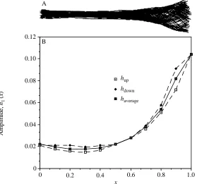
The first example is based on kinematic measurements from a swimming saithe (Videler and Hess, 1984), a subcarangiform swimmer. For this animal, the slope of h1(x)
near the tail end is not equal to zero (Fig. 1). Hess and Videler (1984) noticed the influence of the amplitude slope at the tail end, but still considered a higher efficiency to be more plausible. However, the measurements were highly accurate and the contribution of the term containing the slope at the caudal end should be included in the estimation of thrust and efficiency.
The body dimensions of, and kinematic data on, an ‘average’ saithe needed for the calculation of hydrodynamic quantities are listed in Table 1. The wave speed V (or the wavelength l) measured for the posterior half of the fish is used, as this part of the fish is largely responsible for propulsion. Equation 10 can be written as:
x
1.0 0.8
0.6 0.4
0.2 0
0 0.02 0.04 0.06 0.08 0.10 0.12
Amplitude,
h1
(x
)
B A
where b=U/V and
To determine h19(L), we chose two points, x=L and x=L2DL, at which the amplitude
values are hmand htrespectively. The value of h19(L) is simply obtained from:
giving:
From Table 1, we take b=0.827 and l=1.04L. If we chose DL=0.04L then, from
Fig. 1B, ht=0.076L and hm=0.083L can be estimated, giving a=0.349, h0=0.914 and h=0.673. In the case of the saithe, there is a considerable difference of up to 20% between the calculated values for efficiency obtained with and without a contribution from the slope.
Trout
The second and third examples will use our own kinematic data from two trout (trout 1,
L=0.16m and trout 2, L=0.18m). Their kinematic data are listed in Table 1, in which the
wavelength is obtained by directly measuring the wave form from the centre lines (Webb
[image:5.595.57.427.414.622.2]et al. 1984).
Table 1. Variables for calculation of hydrodynamic quantities and the resulting
efficiencies
Variable Abbreviation Saithe Trout 1 Trout 2
Body length (m) L 0.40 0.16 0.18
Height of caudal fin at trailing edge (L) bt 0.24 0.20 0.20
Half-span (L ) b 0.12 0.10 0.10
Reynolds number Re =UL/n 2×10⁵– 8×10⁵ 0.44×10⁵ 1.2×10⁵
Time period (s) Tt 0.278 0.30 0.21
Swimming speed (L/T) U 0.86 0.516 0.777 Amplitude at the tail end (L) hm 0.083 0.100 0.104 Wave speed (caudal body) (L/Tt) V 1.04 0.864 0.942 Speed ratio (caudal body) β= U/V 0.827 0.598 0.817 Reduced frequency σ = 2p/U 7.302 12.17 8.156 Wave number k =2p/V 6.038 7.269 6.667 Wavelength (caudal body) (L) l 1.04 0.864 0.942
Efficiency without slope term by using EBT h0 0.913 0.799 0.909 Efficiency with slope term by using EBT h 0.673 0.738 0.724 Efficiency by using 3DWPT h 0.602 0.686 0.573 Speed ratio specified by equation 19 bm 0.670 0.652 0.697
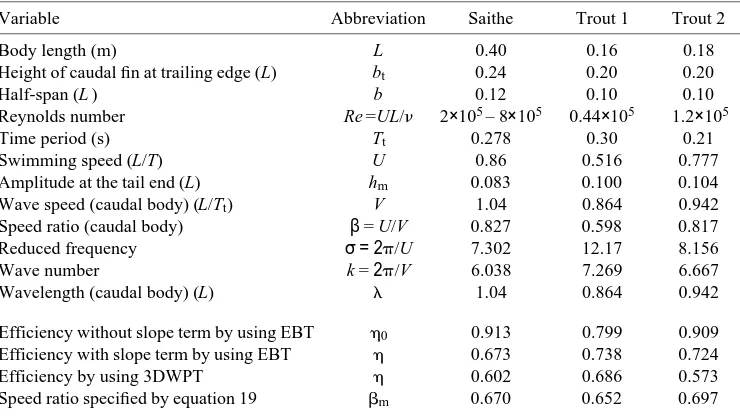
The digitized centre lines of a sequence of movement and the amplitude function of trout 1 are shown in Fig. 2A,B. In one swimming period (Tp=0.38s), 71 centre lines are
digitized. Forty segments are used to construct each line. The non-zero slope near the end of the tail can also be seen. The amplitude distribution shows an asymmetry with respect to the x-axis. The average values of the up and down (left and right movements in reality) amplitudes are plotted in Fig. 2B and will be used in the calculation of locomotory dynamics.
From Table 1, we have b=0.598 and l=0.864L. If we chose DL=0.10L, then ht=0.073L
and hm=0.100L. So a=0.371, h0=0.799 and h=0.738. In this example, the influence of the
actual slope on the calculated efficiency is less pronounced.
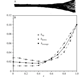
The movement of trout 2 is shown in Fig. 3. Again the average amplitude of up and down movements is used (Fig. 3B). From the table and figure, we have b=0.817,
l=0.942L,DL=0.05L ht=0.092 and hm=0.104L. Hence, a=0.318, h0=0.909 and h=0.724.
The efficiency changes considerably after considering the slope term for trout 2.
Comparison with the three-dimensional unsteady theory and discussion
The three-dimensional waving plate theory (denoted by 3DWPT, Cheng et al. 1991) can be used to obtain a more accurate estimate of the propulsive performance of the examples given above. In this theory, the incompressible potential flow past a flexible
x 0.6 0.8 1.0
0.4 0.2
0 0 0.02 0.04 0.06 0.08 0.10 0.12
hdown hup
haverage
Amplitude,
h1
(x
)
[image:6.595.100.367.346.605.2]B A
thin plate of finite aspect ratio performing a small-amplitude undulatory motion is treated by the linear unsteady vortex ring panel method in the frequency domain. The plate and its wake are replaced by a suitable distribution of vortex rings in a way satisfying the appropriate boundary conditions.
In the calculations we present, the swimming fishes are modelled by rectangular undulating plates (length L and height 2b) corresponding to the centre surfaces of their bodies. The body movement is assumed to be described by equation 7 with amplitude envelopes h1(x) (Figs 1B, 2B and 3B) that are close to exponential functions (Cheng and
Blickhan, 1994). The given parameters are reduced frequency s=vL/U and wave number k=2pL/land the calculated efficiencies are listed in Table 1. It is found that, for each fish, the value of efficiency calculated by 3DWPT is lowest among three results. The efficiency of EBT with the slope term is close to that of 3DWPT, i.e. the slope term should be considered in using EBT for these fishes.
In EBT, the time-averaged propulsive quantities depend only on the events at the caudal end. These estimates are based on the assumption that movement and body shape immediately rostral to the tail end should not be very different (‘slender body’). As shown, the change of movement near the tail tip cannot be neglected for fishes swimming with variable amplitude. The EBT contains a term that approximately considers the influence of the slope. In practice, when determining the slope of the amplitude envelope at the caudal end, a segment as large as the whole tail might be considered.
What is the true efficiency achieved by swimming fishes? The opinion that many
1.0 0.8
0.6 0.4
0.2 0
0 0.02 0.04 0.06 0.08 0.10 0.12
x
A
B
Amplitude,
h1
(x
)
hup
hdown
[image:7.595.87.366.367.628.2]haverage
species swim at efficiencies as high as 90% is based on hydrodynamic calculations. The EBT predicts that a zero slope near the body end is desirable, but this has not been achieved by many fishes, especially those swimming in the subcarangiform mode. For those animals, efficiency should be significantly reduced. Perhaps fishes and cetaceans swimming in the carangiform mode use such a movement pattern and achieve efficiencies of around 90% with lunate fins or flukes.
The increase of the deflection amplitude at the caudal end has an important consequence. If the slope at the tail end is not equal to zero, then efficiency is not simply proportional to b,the ratio of swimming speed to wave speed (Cheng et al. 1991). From equation 15, we can find for a given relative slope aa value of the speed ratio bmat which the efficiency reaches its maximum (see Table 1). Let h/b=0 and considering
b=U/V<1, we have:
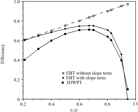
We have used the data from the saithe to see how the efficiency changes with the ratio
bwhen the slope term is included. The wavelength of the waving movement of the body of the fish is almost unchanged when swimming at different speeds for the same fish (Bainbridge, 1963; Webb et al. 1984). Thus, the slope near the tail end of saithe is largely unchanged and the value of aremains constant. The EBT, with the slope term included in the analysis, and 3DWPT give similar results at high values of b, and both depart significantly from the results of EBT without the slope term (Fig. 4). For movement
U/V
Efficiency
EBT without slope term EBT with slope term 3DWPT
1.0 0.8
0.6 0.4
[image:8.595.104.367.387.601.2]0.2 0 0.2 0.4 0.6 0.8 1.0
patterns with variable amplitude, the EBT with the slope term included in the calculations can be considered as suitable for the estimation of swimming performance.
Obviously, both EBT and 3DWPT are limited by their basic assumptions. In order to obtain more precise estimates of hydrodynamic quantities, more realistic fluid-dynamic models are needed.
J.V.C. thanks H. Gebhard, M. Junge, A. Kesel, W. Nachtigall and all the other members of the fish group for their support during his visit to Saarbrücken. J.Y.C. was supported by an Alexander von Humboldt research fellowship, R.B. by a Heisenberg fellowship of the DFG.
References
BAINBRIDGE, R. (1963). Caudal fin and body movements in the propulsion of some fish. J. exp. Biol. 40,
23–56.
BLAKE, R. W.(1983). Fish Locomotion. Cambridge: Cambridge University Press.
BLICKHAN, R., JUNGE, M. ANDNACHTIGALL, W. (1992). Lighthill’s paradox – an artifact? Verh. dt. zool.
Ges. 85, 273.
CHENG, J.-Y. ANDBLICKHAN, R. (1994). Bending moment distribution along swimming fish. J. theor. Biol. (in press).
CHENG, J.-Y., ZHUANG, L.-X. ANDTONG, B.-G. (1991). Analysis of swimming three-dimensional waving plates. J. Fluid Mech. 232, 341–355.
HESS, F. ANDVIDELER, J. J. (1984). Fast continuous swimming of saithe (Pollachius virens): a dynamic analysis of bending moments and muscle power. J. exp. Biol. 109, 229–251.
LIGHTHILL, M. J.(1960). Note on the swimming of slender fish. J. Fluid Mech. 9, 305–317.
LIGHTHILL, M. J.(1975). Mathematical Biofluiddynamics. Philadelphia: SIAM.
TANG, J. ANDWARDLE, C. S. (1992). Power output of two sizes of Atlantic salmon (Salmo salar) at their maximum sustained swimming speeds. J. exp. Biol. 166, 33–46.
VIDELER, J. J. AND HESS, F. (1984). Fast continuous swimming of two pelagic predators, saithe
(Pollachius virens ) and mackerel (Scomber scombrus): a kinematic analysis. J. exp. Biol. 109, 209–228.
VIDELER, J. J. ANDWARDLE, C. S. (1978). New kinematic data from high speed cine film recordings of
swimming cod (Gadus morhua). Neth. J. Zool. 28, 465–484.
WEBB, P. W. (1975). Hydrodynamics and energetics of fish propulsion. Bull. Fish. Res. Bd Can. 190, 1–159.
WEBB, P. W., KOSTECKI, P. T. ANDSTEVENS, E. D. (1984). The effect of size and swimming speed on locomotion kinematics of rainbow trout. J. exp. Biol. 109, 77–95.
WU, T. Y. (1971). Hydrodynamics of swimming fishes and cetaceans. Adv. appl. Math. 11, 1–63. YATES, G. T. (1983). Hydromechanics of body and caudal fin propulsion. In Fish Biomechanics