Electric organ discharges and electric images during electrolocation

Two orders of teleost fish, the Gymnotiformes from South America and the Mormyroidei in Africa, have independently evolved capabilities to generate and sense electric fields, called electrogenesis and electroreception (for reviews, see Bullock and Heiligenberg, 1986; Carr, 1990). Electric discharges (EODs) generated by a specialized electric organ (EO) within the body cause electric current to flow in the surrounding water. Nearby objects with a different electrical impedance from that of water alter the current flowing through sensory electroreceptor organs in the fish’s skin. Electric fish can locate and identify, or electrolocate, nearby objects, on the basis of the spatial and temporal patterns of transdermal potential perturbations called electric images.

Since the discovery of electroreception in the 1950s, great progress has been made in studies of electric fish and the central neurophysiology of electrosensory systems. However, the specific algorithms and neuronal computations involved in active electrolocation are still largely unknown. Understanding how electric fish perceive objects from electric images is difficult, in part because electric images are generally complex functions of object and EOD geometry, and also because

electrolocation is performed through a variety of behaviors that are difficult to maintain in electrophysiological preparations. The fish’s normal movements change the EO source locations and the orientation of the electroreceptor array relative to external objects, and therefore greatly affect the sequence of electric images. Presumably the fish employ behavioral strategies to enhance the information available in the peripheral electrosensory image. However, this hypothesis has not been fully tested because the electrosensory input has not yet been well described during exploratory behaviors in freely moving fish.

Quantifying the pattern of electrosensory stimuli is a crucial step in studying electrosensory information processing and understanding electrolocation at algorithmic and neuronal levels. How is the electric image of the fish’s environment formed? Can we predict changes in the electric field from objects and during natural behaviors? Do the behaviors have significant sensory consequences and thus reflect the animal’s particular strategies or computational requirements?

To answer these questions, we have focused on reconstructing quantitatively the entire pattern of currents JEB2079

Weakly electric fish use active electrolocation – the generation and detection of electric currents – to explore their surroundings. Although electrosensory systems include some of the most extensively understood circuits in the vertebrate central nervous system, relatively little is known quantitatively about how fish electrolocate objects. We believe a prerequisite to understanding electrolocation and its underlying neural substrates is to quantify and visualize the peripheral electrosensory information measured by the electroreceptors. We have therefore focused on reconstructing both the electric organ discharges (EODs) and the electric images resulting from nearby objects and the fish’s exploratory behaviors. Here, we review results from a combination of techniques, including field measurements, numerical and

semi-analytical simulations, and video imaging of behaviors. EOD maps are presented and interpreted for six gymnotiform species. They reveal diverse electric field patterns that have significant implications for both the electrosensory and electromotor systems. Our simulations generated predictions of the electric images from nearby objects as well as sequences of electric images during exploratory behaviors. These methods are leading to the identification of image features and computational algorithms that could reliably encode electrosensory information and may help guide electrophysiological experiments exploring the neural basis of electrolocation.

Key words: electrolocation, electroreception, electric organ discharge, Gymnotiformes, electric fish.

Summary

Introduction

ELECTRIC ORGAN DISCHARGES AND ELECTRIC IMAGES DURING

ELECTROLOCATION

CHRISTOPHER ASSAD1,_{*, BRIAN RASNOW}2,_{† ANDPHILIP K. STODDARD}3

1_{Department of Electrical Engineering and} 2_{Division of Biology, California Institute of Technology, Pasadena,}

CA 91125, USA and 3Department of Biological Sciences, Florida International University, Miami, FL 33199, USA *Present address: Jet Propulsion Laboratory, MC 303-300, 4800 Oak Grove Drive, Pasadena, CA 91109, USA

(e-mail: Chris.Assad@jpl.nasa.gov)

†Present address: Amgen Inc., One Amgen Center Drive, Thousand Oaks, CA 91320, USA

resulting from the fish’s discharge and environment. Because electrosensory input patterns are highly dependent on the EOD pattern, we have re-examined in detail the autogenous EODs. In the first section below, we present and interpret EOD maps for several gymnotiform species. In the second section, we describe computer simulations designed to reconstruct electric images resulting from external objects and the fish’s exploratory behaviors. Electric images depend on many variables, including the fish’s EOD, the electrical impedance of its body and skin, water resistivity, the impedance and geometry of the object and the location, configuration and velocity of the body and object. We have used semi-analytical simulations of static electric images to propose algorithms for extracting sets of object features (e.g. their size, distance, impedance, shape) from sets of electric image features (e.g. position, amplitude, spread, phase). To examine natural dynamic behaviors and to predict sequences of electric images from electric fish exploring novel objects, we have developed a more general three-dimensional electric field simulator. Our results suggest how the fish’s probing movements could help it recognize object features. Our detailed field maps and electric field simulators are powerful new tools for exploring the neurocomputational algorithms for electrolocation. In the final section below, we discuss an electrolocation model based on feature sets and algorithms revealed by systematic analyses of electric images. The preliminary model and its predictions may help guide electrophysiological experiments exploring the neural basis of electrolocation.

Electric organ discharges

Electric organ discharges are generally classified by voltage waveforms measured between electrodes near the fish’s head and tail: ‘wave’ fish produce continuous, periodic discharges, while ‘pulse’ fish have silent intervals between discharges. The head-to-tail waveforms are highly stereotypical for each species (Bennett, 1971; Bass, 1986). Far from the fish, the spatial pattern of the EOD has dipolar geometry, but the near field can be quite complicated and ‘far from dipole-like’ (Knudsen, 1975). Waveforms recorded at different locations near the body surface often vary significantly from the head-to-tail waveform (Bennett, 1971; Watson and Bastian, 1979; Hoshimiya et al., 1980; Bastian, 1986; Rasnow et al., 1993), particularly in species with long electric organs and high-frequency components. Because electrolocation occurs in the near field (Bastian, 1986), these local variations are probably important for electrolocation. They also make it difficult to visualize the EOD pattern.

We have developed a powerful system for mapping EOD potentials and electric field vectors in three dimensions. Using a robotic positioning arm, we digitized the EOD of a stationary fish at hundreds of positions around its body. Potential waveforms were recorded relative to a distant reference electrode, and potential gradients (proportional to electric field components) were recorded differentially between nearby pairs of electrodes. Because we also digitized EODs simultaneously

on a stationary reference electrode, we were able to time-align the multiple records with submicrosecond precision. Slices taken through the aligned EOD records in time and space can be visualized as maps by interpolating and rendering instantaneous potential and field amplitudes in pseudocolor or grayscale (Rasnow et al., 1993; Rasnow and Bower, 1996; Assad et al., 1998).

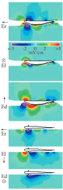
To date we have mapped the EODs of three gymnotiform wave species and seven gymnotiform pulse species. These maps, for the first time, clearly illustrate the full spatiotemporal structure of the EOD (Fig. 1). In the majority of species, the EOD waveforms vary greatly with location, revealing considerably more complex patterns than were previously appreciated. In addition to displaying complex spatiotemporal patterns of amplitude, field direction, direct-current bias, phase and harmonic composition, the EOD maps have revealed many other and sometimes unexpected features. These include: (1) the location of the EO within the body, correlated with areas of greatest amplitude; (2) functional segmentation of the EO, correlated with localized peaks and their spatiotemporal pattern; (3) the range of electrolocation, correlated with the separation and strengths of the sources and far-field amplitude; (4) the effectiveness of EO synchronization mechanisms, correlated with the spatiotemporal pattern of the EOD peaks along the body and local spectra; and (5) suggested phylogenetic relationships.

The maps, in the form of pseudocolor animated EOD movies, are available through the Internet (www.bbb.caltech.edu/ ElectricFish and www.fiu.edu/stoddard/electricfish.html), and highlights for several species are briefly summarized as follows.

Eigenmannia virescens (Valenciennes, 1847)

The lowest-frequency wave fish of the species mapped, Eigenmannia virescens, has a simple EOD that resembles an oscillating dipole. Amplitude peaks reveal the ventral location of the EO (Assad et al., 1998). Synchronized activation along the length of the electric organ implies effective mechanisms for compensation of neuronal propagation delays along the length of the EO (Bennett, 1971). Eigenmannia exhibits a strong jamming avoidance response (JAR), whereby the fish shifts its EOD frequency to avoid interference from the EOD of a neighbor that would degrade electrolocation performance (Heiligenberg, 1991). The JAR relies on EOD comparisons across different body regions, with performance proportional to the surface area, and so may be facilitated by a spatially uniform EOD. In other species with highly variable local field waveforms, the effects of a jamming signal change with location on the body, possibly making direct comparisons across regions more difficult.

suggesting that segments of the electric organ are active sequentially instead of synchronously (Rasnow et al., 1993). The 5–10 cm ms−1 _{velocity of the peaks along the tail is} consistent with the expected conduction velocity of the spinal relay axons driving the electric organ (Lorenzo et al., 1990). The electric field vector in the caudal 50–75 % of Apteronotus spp. also rotates during the EOD cycle (Rasnow and Bower, 1996), whereas rostral of the pectoral fin, the field magnitude

and sign oscillate while maintaining relatively constant orientation.

Brachyhypopomus sp. (soon to be named B. walteri by J. P. Sullivan) and B. Beebei (Schultz, 1944)

The slow biphasic pulse EOD (4 ms) of Brachyhypopomus sp. begins with a widely spaced dipole in the rostral body, which strengthens for 0.5 ms before propagating caudally with

sp.

2 ms

constant pole spacing. B. beebei has a faster biphasic EOD (1 ms), with very rapid phase transitions. In contrast to that of Brachyhypopomus sp., the EOD of B. beebei begins as an initial weak dipole between the mouth and anus, with a considerable current component flowing dorso-ventrally. The EOD then fragments into multipoles as it propagates towards the tail, implying incomplete or heterogeneous EO propagation delay compensation (Stoddard et al., 1995). B. pinnicaudatus (Hopkins, 1991) produces an EOD twice as long but similar in most other respects to that of B. beebei, its closest known relative (Sullivan, 1997). In both species, EODs of males have an extended recovery of the second phase, whereas the female’s EODs are symmetrical around 0 V. However, the spatial activation patterns of the two sexes are virtually identical (Stoddard et al., 1999). In all three Brachyhypopomus species mapped, the sources and sinks of the initial head-positive phases are located more rostral than those of subsequent head-negative phases. This spatial offset of activation is consistent with rostral electrocytes first firing on their posterior face, producing the head-positive phase, but only the caudal subset of electrocytes firing on their non-innervated anterior face, producing the head-negative phase (Bennett, 1971). This pattern of EO activation reduces the dipole moment and spatial extent of the time-averaged far field, perhaps to mask the EOD from ampullary electroreceptive predators (Stoddard, 1994). Furthermore, the asymmetric activation results in a positive direct current field at the head, which is proportional to the EOD pulse rate and which increases during exploratory behaviors. The polarity of this direct current biasing suggests that active electrolocation might be possible with the ampullary system (Stoddard et al., 1995), which could have both evolutionary and behavioral significance.

Gymnotus carapo (L.)

The multiphasic head-to-tail waveform is a mere shadow of the elaborate EOD spatiotemporal pattern (B. Rasnow, P. K. Stoddard and C. Assad, in preparation). The EOD begins with a long-lasting weak dipolar phase in the ventral portion of the head, with the dipole axis tilted approximately 30 ° out of the horizontal plane. After this initial prepulse, the EOD becomes very complicated and rapidly changing, reflecting a complicated and heterogeneous electric organ (Trujillo-Cenóz and Echagüe, 1989). Substantial currents between the dorsal and ventral sides of the body result from the ventral location of the EO and differential activity between the EO tubes (Caputi and Aguilera, 1996) (Fig. 2). The complex EO activation with path-length compensation (Lorenzo et al., 1990) creates the largest separation between the positive and negative peaks seen in any of these fish. Two other South American species, G. podanopterus Leccia, 1994) and G. coatesi (Mago-Leccia, 1994), have very similar EOD patterns, but a Central American species, G. cylindricus (LaMonte, 1935), has instead a simple monophasic EOD with no direct current offset (B. Rasnow, P. K. Stoddard and C. Assad, in preparation). This primitive EOD appears more similar to the EOD produced by

Hunter’s organ in the electric eel Electrophorus electricus (L.), suggesting a close phylogenetic relationship between the two species.

Although many of the spatial and temporal EOD features displayed here could, in principle, convey useful information for electrolocation, we do not know which actually do and which may serve other purposes or even be unimportant artifacts of controlling elongated electric organs. These questions can be addressed by exploring the electrosensory consequences of the rich EOD field, as in the following sections.

Reconstructing electric images of objects and electrosensory consequences of exploratory behaviors

How might electric fish identify object features, such as size, shape, location or velocity, from the object’s electric images? How do fish differentiate between large, distant objects and small, nearby ones, or between large objects with an impedance similar to that of water and smaller objects with a greater differential impedance? To answer these and related

questions, we begin by exploring how geometrically simple objects distort the field pattern and cast electric images onto the electroreceptive surface. We proceed to explore how electric images change during exploratory behaviors.

Previous electrolocation experiments have examined the electrosensory stimuli and the electroreceptor responses from nearby objects, but independently from natural exploratory behaviors. For example, Bastian (1981) measured the change in the root mean square (RMS) EOD potential, together with single-unit electroreceptor responses, after moving conductive and insulating spheres and cylinders at different distances from A. albifrons. He showed that electric image amplitudes generally have different functional dependencies on object distance, size and velocity, so in principle a fish could resolve these quantities by actively varying the distance and velocity. However, the animals were necessarily held in a fixed position, usually curarized and respirated. In the behavioral experiments that have been reported, there were no field measurements or physiology to avoid interference with the natural behaviors (e.g. Toerring and Belbenoit, 1979; Behrend, 1984; Knudsen, 1974; Heiligenberg, 1973; Lissmann, 1963). These two types of experiments need to be bridged in order to study the electrosensory consequences of exploratory behaviors.

Movements of the fish result in significant changes in the sensory input, both in the object image and from the movement itself, a consequence termed sensory reafference (von Holst and Mittelstaedt, 1950). Distinguishing sensory exafference from reafference is critical to the success of active electrolocation (Heiligenberg and Bastian, 1984). For example, tail bending changes the field strength near the rostral body by a few per cent (Bastian, 1995), which can easily mask the weaker electric images typical of small objects (Assad, 1997). Many species, especially those with long electric organs, swim by undulating only a single elongated ventral or dorsal fin, while at the same time holding their bodies rigid (Lissmann, 1963; Behrend, 1984). This allows the fish to swim equally well forwards or backwards and to hold the body in an arc around objects (Bastian, 1986; Toerring and Belbenoit, 1979) while maintaining rigid control over the electroreceptive surfaces. Presumably, by keeping the detector array in a fixed orientation with respect to field generation, this controlled body motion reduces the number of variables that must be taken into account to interpret electrosensory information.

Simulations provide a non-invasive way to study natural exploratory behaviors and provide an efficient means of quantifying the electrosensory images caused by small objects. However, all simulation methods involve trade-offs between accuracy, precision, conceptual simplicity and computational efficiency. We have therefore developed two different electric image simulators, using a three-dimensional semi-analytical approach based on the measured fields (Rasnow, 1996), and a more general three-dimensional boundary element numerical method (BEM; Assad, 1997). These improved methods were a logical step in a progression made clear from previous electric fish modeling efforts, which produced interesting

results from two-dimensional difference and finite-element simulations (Heiligenberg, 1975; Hoshimiya et al., 1980) and from a three-dimensional analytical model (Bacher, 1983). We have added resolution to the spatial and temporal dimensions, both of which are essential to understanding how this sensory modality works.

Electric images

Quantitatively accurate electric images of small elliptical objects can be directly computed from electric field vectors (EOD maps) measured without the object (Rasnow, 1996). The electric images resulting from this semi-analytical simulator have 1–3 phase potential ‘bumps’ across the body, bumps that are weak and broad (no high spatial frequencies) (Fig. 3; Rasnow, 1996; Bacher, 1983; Heiligenberg, 1975). A systematic analysis suggested the following mapping between sensory image features and corresponding physical features of

∆

mV RMS

0 0.1 0.2 0.3

4 6 8 10

Distance from head (cm) ...

.

...

∆

mV RMS

.

...

0 0.1 0.2 0.3

4 6 8 10

A

B

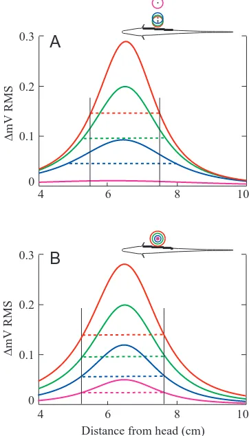
the objects. The location of the phase-averaged (e.g. RMS) image peak coincides with the object’s position over the body surface and thus unambiguously reveals two of the object’s three spatial position coordinates. Because the peak amplitude of the image is affected by multiple object parameters (its size, shape, distance and impedance), the object’s distance depends on more than one image parameter. A simple solution to distinguish a spherical object’s distance from its size is that the relative spatial width of the image (i.e. a parameter like the standard deviation of a Gaussian function) depends solely, and linearly, on the distance to the sphere’s center, and is independent of the sphere’s size (Fig. 3). Object impedance can be extracted from the image polarity and relative phase of the EOD and the electric image. Finally, object size can be determined unambiguously from the distance, the impedance and the peak amplitude of the image, the latter being proportional to the sphere’s volume. These results are summarized in Fig. 4 (for details, see Rasnow, 1996).

Applying the same algorithm to nonspherical ellipsoids resulted in false perceptions of spheres whose proximal surface distance and shape corresponded with the proximal surface of the ellipsoids (Rasnow, 1996). Because the EOD attenuates steeply with distance from the fish, the nearest or proximal parts of the object will contribute disproportionately to the electric image. The resulting distortion, somewhat analogous to perspective distortion inherent in wide-angle optical lenses, might make discrimination of object shape a more complicated task. Tail bending, and phase information in fish with rotating EOD vectors, could contribute to depth perception. For example, electric images of a conductor will be largest when the EOD field is oriented parallel to the major axis because a larger region of water is short-circuited. Thus, tail bending and EOD phase could reveal object asymmetry in a manner crudely analogous to how an object’s shadow depends on illumination angle. Phase information is also necessary to resolve an object’s impedance. Although the model has thus far been applied only to Apteronotus, it should prove informative to examine and compare object images using the EOD patterns of the other species.

The major advantages of the semi-analytical three-dimensional simulator are computational simplicity (relative to the BEM), and the additional intuition provided by analytical (compared with purely numerical) solutions. However, electric images are limited to the proximal side of the body because

the method does not account for the secondary effects of the body on the object perturbation, and simulations require the electric field vector be measured at object locations with the same body configuration. To address these limitations and to simulate exploratory behaviors further, we built a complementary three-dimensional BEM electric fish model.

Exploratory behaviors during electrolocation

The BEM simulator uses a more general and complicated numerical method that can model the fish in any body position (Assad, 1997; C. Assad and J. M. Bower, in preparation). The method requires only surfaces and boundaries to be defined and covered by nodes and elements. After conductivities have been added and sources have been chosen inside the body to represent the EO, the electric potential and normal currents are solved for at each node, and potentials at arbitrary exterior points can then be computed. The model was calibrated by matching its output to measured EOD maps and validated by comparison with analytical methods. For example, in Fig. 5, the simulator produces the expected dipolar distortion from a spherical object near the tail of Apteronotus albifrons. The major advantages of the BEM are that the tail and body can be bent, arbitrarily shaped objects can be included by adding nodes across their surfaces, and the model accounts for secondary effects of the fish’s body on the EOD and electric images. A disadvantage is sensitivity to parameters describing the EO and the impedances of the skin and body.

Electric image features Object features Peak location

Relative size (width) Peak amplitude Sign and phase

Phasic images

Rostrocaudal location Distance

Size

Shape

Conductivity and dielectric constant

Fig. 4. The mapping between sensory electric images and the external environment is sufficient to locate and identify small homogeneous objects.

A

B

Fig. 5. Example boundary element numerical method (BEM) simulation results from a tail-scanning behavior of Apteronotus

leptorhynchus. (These results can also serve to represent the EOD of A. albifrons in the second and third frames of Fig. 6, because the

We have used the BEM simulator to analyze video-taped data of A. albifrons ‘scanning’ objects (Fig. 6) and to analyze a ‘tail-probing’ behavior of Eigenmannia (Assad, 1997). These scanning and tail-probing behaviors have been described previously (Lissmann, 1963; Heiligenberg, 1975; Toerring and Belbenoit, 1979; Bacher, 1983; Behrend, 1984; Bastian, 1986). Two common hypotheses were drawn from these studies. First, many electric fish scan and swim with rigid control of the spine and body posture, which should maintain the relative orientation of field generator to field receptors and so reduce undesirable reafferent modulations. Our video and simulation results strongly support this conclusion. The scanning or probing movements have also been hypothesized to help recognize object features. For example, Heiligenberg’s (1975) relatively coarse finite difference simulation showed that tail bending may help increase spatial contrast, and Bacher’s (1983) analytical three-dimensional model led him to suggest that tail bending could separate object shape from position. The BEM simulation results indicate that electric fish do control their movements to regulate the electrosensory input. For example, in the Eigenmannia tail-probing behavior, the fish’s specific

movements modulate the amplitude of the object image while maintaining a stable image pattern on the rostral body surface (Assad, 1997), perhaps allowing the fish to disambiguate object features. The sensory and computational significance of these behaviors will be reported shortly (C. Assad and J. M. Bower, in preparation).

Neurocomputational algorithms

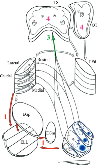
Ultimately, weakly electric fish must extract and interpret any useful signals contained in small-field perturbations superimposed upon the intrinsic EOD pattern. Therefore, a considerable volume of the electric fish brain is devoted to electrosensory processing. For the computational algorithms proposed above to be involved in electrolocation, they must have a plausible neural implementation in the fish’s nervous system. We propose one such projection onto the neural networks in the electric fish brain. Fig. 7 summarizes the gymnotiform fish’s electrosensory pathways and central processing structures (Carr and Maler, 1986). The electrosensory lateral line lobe (ELL) receives the raw peripheral field encoded by the transdermal electroreceptors in

µV

µV

multiple somatotopically organized maps (Carr and Maler, 1986). The first processing step may be to extract the object’s image. This could be done in the ELL by descending feedback and gain control (labeled 1 in Fig. 7), which is capable of subtracting out the expected EOD (Bell et al., 1997; Bastian, 1996). The algorithms suggest that relative image size (spatial width of the peak) is the next calculation. Cells in the ELL maps have center-surround-type receptive fields. Convolving the object’s image with center-surround spatial filters, and applying a threshold, results in an area of activity proportional to the image size (labeled 2 in Fig. 7). The object distance can be calculated by integrating over this active area. Such integration could be achieved within the convergent projections from the ELL onto higher areas (labeled 3 in Fig. 7). Although the ELL projects to both the dorsal preeminential nucleus and the torus semicircularis (TS), the

former is part of the feedback loop to compute object images in the ELL. Therefore, this scenario predicts that object distance may first be represented unambiguously in the amplitude pathway input layers of the torus. In particular, toral or tectal neurons might respond similarly to large and small spheres centered at the same positions (and perhaps even ellipsoids at the corresponding locations), even though the electroreceptor responses in these cases would be quite different. Consistent with this hypothesis, tuning to object distance has been observed in the optic tectum (Bastian, 1986). Finally, knowing object distance is a prerequisite (or corequisite) in the model for deconfounding size, impedance and shape, so these features would first appear in the torus and higher areas. Although this proposal is not yet based on quantitative simulation or modeling, we believe it may be a useful working hypothesis for interpreting and further exploring parts of the electrosensory nervous system.

Conclusions and future directions

These computational algorithms help predict the encoding and transformations of electrosensory information. They suggest how important object features that are confounded and ambiguous in the sensory input may emerge at successive levels of the nervous system. The algorithms can be refined, tested and generalized on the basis of the data and simulations outlined above to arrive at a robust working model of electrolocation.

Research on electric fish has focused recently on the JAR, on descending feedback to the ELL and on other topics more amenable to electrophysiological investigation than electrolocation. Making sense of the complex relationships between object features and neuronal responses is extremely difficult without quantitative models that encapsulate the nonlinearities between object features and peripheral electrosensory images. The models proposed here may therefore stimulate renewed experimental interest in the neural basis of electrolocation. In particular, simulations of peripheral electrosensory images, coupled with models of electroreceptor transfer functions, can produce accurate afferent input patterns to the ELL. These ascending patterns should help to elucidate both the descending input and the neural computations within the ELL. Electrolocation algorithms also lay the groundwork for electrophysiological studies at higher levels of the nervous system, for example, by predicting specific emergent features in the midbrain and cerebellum.

Much of this work was performed in the laboratory of James M. Bower. Rachel Hunter and Maritza Alvarado assisted with the behavioral experiments. Mark Kilburn assisted in mapping the EODs of B. pinnicaudatus and G. cylindricus. Melita Morton and Duanne Jones assisted in raising the pulse fish to maturity. Financial support came from NSF grant IBN-9319968 to J.M.B., FIU Foundation and NIH/NIGMS-GM08205-11 grants to P.K.S. and JPL/CISM to C.A.

Lateral

Caudal

EGm EGp

ELL

Rostral

Medial

OT TS

PEd

References

Assad, C. (1997). Electric field maps and boundary element

simulations of electrolocation in weakly electric fish. PhD thesis, California Institute of Technology, Pasadena, CA. University Microfilms Inc., Ann Arbor, MI.

Assad, C., Rasnow, B., Stoddard, P. K. and Bower, J. M. (1998).

The electric organ discharges of the gymnotiform fishes. II.

Eigenmannia. J. Comp. Physiol. A 183, 419–432.

Bacher, M. (1983). A new method for the simulation of electric fields,

generated by electric fish and their distorsions by objects. Biol.

Cybernetics 47, 51–58.

Bass, A. H. (1986). Electric organs revisited: evolution of a vertebrate

communication and orientation organ. In Electroreception (ed. T. H. Bullock and W. Heiligenberg), pp. 13–70. New York: Wiley.

Bastian, J. (1981). Electrolocation. I. How the electroreceptors of Apteronotus albifrons code for moving objects and other electrical

stimuli. J. Comp. Physiol. 144, 465–479.

Bastian, J. (1986). Electrolocation: behavior, anatomy and physiology. In Electroreception (ed. T. H. Bullock and W. Heiligenberg), pp. 577–612. New York: Wiley.

Bastian, J. (1995). Pyramidal-cell plasticity in weakly electric fish: a

mechanism for attenuating responses to reafferent electrosensory inputs. J. Comp. Physiol. A 176, 63–78.

Bastian, J. (1996). Plasticity in an electrosensory system. I. General

features of a dynamic sensory filter. J. Neurophysiol. 76, 2483–2496.

Behrend, K. (1984). Cerebellar influence on the time structure of

movement in the electric fish Eigenmannia. Neurosci. 13, 171–178.

Bell, C. C., Bodsnick, D., Montgomery, J. and Bastian, J. (1997).

The generation and subtraction of sensory expectations within cerebellum-like structures. Brain Behav. Evol. 50 (suppl. 1), 17–31.

Bennett, M. V. L. (1971). Electric organs. In Fish Physiology, vol. 5

(ed. W. S. Hoar and D. J. Randall), pp. 347–491. New York: Academic Press.

Bullock, T. H. and Heiligenberg, W. (1986). (eds) Electroreception.

New York: Wiley.

Caputi, A. and Aguilera, P. (1996). A field potential analysis of the

electromotor system in Gymnotus carapo. J. Comp. Physiol. 179, 827–835.

Carr, C. E. (1990). Neuroethology of electric fish. Bioscience 40,

259–267.

Carr, C. E. and Maler, L. (1986). Electroreception in gymnotiform

fish. In Electroreception (ed. T. H. Bullock and W. Heiligenberg), pp. 319–373. New York: Wiley.

Ellis, M. M. (1912). The freshwater fishes of British Guiana,

including a study of the ecological groupings of species and the relation of the fauna of the Plateau to that of the Lowlands (ed. C. H. Eigenmann). Mem. Carnegie Mus. 5, 1–578.

Heiligenberg, W. (1973). Electrolocation of objects in the electric

fish Eigenmannia. J. Comp. Physiol. 87, 137–164.

Heiligenberg, W. (1975). Theoretical and experimental approaches to

spatial aspects of electrolocation. J. Comp. Physiol. 103, 247–272.

Heiligenberg, W. (1991). Neural Nets in Electric Fish. Cambridge,

MA: MIT Press.

Heiligenberg, W. and Bastian, J. (1984). The electric sense of

weakly electric fish. Annu. Rev. Physiol. 46, 561–583.

Hopkins, C. D. (1991). Hypopomus pinnicaudatus (Hypopomidae),

a new species of gymnotiform fish from French Guiana. Copeia

1991, 151–161.

Hoshimiya, N., Shogen, K., Matsuo, T. and Chichibu, S. (1980).

The Apteronotus EOD field: waveform and EOD simulation. J.

Comp. Physiol. 135, 283–290.

Knudsen, E. (1974). Behavioral thresholds to electric signals in high

frequency electric fish. J. Comp. Physiol. 91, 333–353.

Knudsen, E. (1975). Spatial aspects of the electric fields generated

by weakly electric fish. J. Comp. Physiol. 99, 103–118.

LaMonte, F. (1935). Two new species of Gymnotus. Am. Mus. Novitates 781, 1–3.

Lissmann, H. W. (1963). Electric location by fishes. Scient. Am. 208,

50–59.

Lorenzo, D., Sierra, F., Silva, A. and Macadar, O. (1990). Spinal

mechanisms of electric organ synchronization in Gymnotus carapo.

J. Comp. Physiol. A 167, 447–452.

Mago-Leccia, F. (1994). Electric Fishes of the Continental Waters of America. Biblioteca de la Academia de Ciencias Fisicas,

Matematicas y Naturales. vol. XXIX. Caracas, Venezuela.

Rasnow, B. (1996). The effects of simple objects on the electric

field of Apteronotus leptorhynchus. J. Comp. Physiol. A 178, 397–411.

Rasnow, B., Assad, C. and Bower, J. M. (1993). Phase and

amplitude maps of the electric organ discharge of the weakly electric fish, Apteronotus leptorhynchus. J. Comp. Physiol. A 172, 481–491.

Rasnow, B. and Bower, J. M. (1996). The electric organ discharges

of the gymnotiform fishes. I. Apteronotus leptorhynchus. J. Comp.

Physiol. A 178, 383–396.

Schultz, L P. (1944). Two new species of fishes (Gymnotidae,

Loricariidae) from Caripito, Venezuela. Zoologica 29, 39–44.

Stoddard, P. K. (1994). Low frequency electric field production and

concealment in gymnotiform fish with pulsed electric organ discharges. Soc. Neurosci. Abstr. 24, 370.

Stoddard, P. K., Rasnow, B. and Assad, C. (1995). Electric organ

discharges of the gymnotiform fish Brachyhypopomus spp. In

Nervous Systems and Behavior, Proceedings of the 4th

International Congress of Neuroethology (ed. M. Burrows, T. Matheson, P. L. Newland and H. Schuppe), p. 417. New York: Theimme Medical Publishers.

Stoddard, P. K., Rasnow, B. and Assad, C. (1999). The electric

organ discharges of the gymnotiform fishes. III. Brachyhypopomus.

J. Comp. Physiol. A (in press).

Sullivan, J. P. (1997). A phylogenetic study of the neotropical

hypopomid electric fishes (Gymnotiformes: Rhamphichthyoidea). Doctoral dissertation, Duke University.

Toerring, M. J. and Belbenoit, P. (1979). Motor programmes and

electroreception in mormyrid fish. Behav. Ecol. Sociobiol. 4, 369–379.

Trujillo-Cenóz, O. and Echagüe, J. A. (1989). Waveform

generation of the electric organ discharge in Gymnotus carapo. I. Morphology and innervation of the electric organ. J. Comp.

Physiol. 165, 343–351.

Valenciennes, A. (1847). Poissons. In D’Orbigny Voyage dans l’Amerique Meridionale, vol. 5, part 2. Paris: Librería de los

Señores Gide.

von Holst, E. and Mittelstaedt, H. (1950). Das Reafferenzprinzip. Naturwissenschaften 37, 464–476.

Watson, D. and Bastian, J. (1979). Frequency response characteristics of electroreceptors in the weakly electric fish,