How to Choose Interesting Points for Template
Attacks More Effectively?
Guangjun Fan1, Yongbin Zhou2, Hailong Zhang2, Dengguo Feng1
1 State Key Laboratory of Computer Science, Institute of Software,
Chinese Academy of Sciences
[email protected],[email protected]
2 State Key Laboratory of Information Security,
Institute of Information Engineering, Chinese Academy of Sciences
[email protected],[email protected]
Abstract. Template attacks are widely accepted to be the most power-ful side-channel attacks from an information theoretic point of view. For template attacks to be practical, one needs to choose some special sam-ples as the interesting points in actual power traces. Up to now, many different approaches were introduced for choosing interesting points for
template attacks. However, it isunknownthat whether or not the
previ-ous approaches of choosing interesting points will lead to the best clas-sification performance of template attacks. In this work, we give a neg-ative answer to this important question by introducing a practical new approach which has completely different basic principle compared with all the previous approaches. Our new approach chooses the point whose distribution of samples approximates to a normal distribution as the in-teresting point. Evaluation results exhibit that template attacks based on the interesting points chosen by our new approach can achieve obvious better classification performance compared with template attacks based on the interesting points chosen by the previous approaches. Therefore, our new approach of choosing interesting points should be used in prac-tice to better understand the practical threats of template attacks.
Keywords: Side-Channel Attacks, Power Analysis Attacks, template attacks, Interesting Points.
1
Introduction
Power analysis attacks have received such a large amount of attention be-cause they are very powerful and can be conducted relatively easily. Therefore, let us focus exclusively on power analysis attacks. As an important method of power analysis attacks, template attacks were firstly proposed by Chari et al. in 2002 [1] and belong to the category of profiled side-channel attacks. Under the assumption that one (an actual attacker or an evaluator) has a reference device identical or similar to the target device, and thus be well capable of character-izing power leakages of the target device, template attacks are widely accepted to be the strongest side-channel attacks from an information theoretic point of view [1]. We note that, template attacks are also important tools to evaluate the physical security of a cryptographic device.
Template attacks consist of two stages. The first stage is the profiling stage and the second stage is the extraction stage. In the profiling stage, one captures some actual power traces from a reference device identical or similar to the target device and builds templates for each key-dependent operation with the actual power traces. In the extraction stage, one can exploit a small number of actual power traces measured from the target device and the templates obtained from the profiling stage to classify the correct (sub)key.
1.1 Motivations
Note that for real-world implementation of cryptography devices, a side-channel leakage trace (i.e. an actual power trace for the case of power analysis attacks) usually contains multiple samples corresponding to the target intermediate val-ues. The reason is that the key-dependent operations usually take more than one instruction cycles. In addition, according to Nyquist-Shannon sampling theorem, the acquisition rate of the signal acquisition device is always set to be several times faster than the working frequency of the target cryptographic device.
For template attacks to be practical, it is paramount that not all the samples of an actual power trace are part of the templates. To reduce the number of samples and the size of the templates, one needs to choose some special points as the interesting points in actual power traces. Main previous approaches of choosing interesting points for template attacks can be divided into two kinds.
introduced. These approaches are Correlation Power Analysis based approach (Chapter 6 in [11]) (CPA), Sum Of Squared pairwise T-differences based ap-proach [10] (SOST), Difference Of Means based approach [1] (DOM), Sum Of Squared Differences based approach [10] (SOSD), Variance based approach [16] (VAR),Signal-to-Noise Ratios based approach(pp. 73 in [11]) (SNR),Mutual In-formation Analysis based approach [17] (MIA), andKolmogorov-Smirnov Anal-ysis based approach [18] (KSA). One uses these approaches to choose the points which contain the most information about the characterized key-dependent oper-ations as the interesting points by computing the signal-strength estimateSSE(t) for each pointPt. For example, when one uses Correlation Power Analysis based approach to choose interesting points for template attacks, the signal-strength estimateSSE(t) is measured by the coefficient of correlation between the actual power consumptions and the hypothetical power consumptions of a pointPt. For these approaches, in each clock cycle, the point with the strongest signal-strength estimateSSE(t) is chosen as the interesting point.
Approaches belong to the second kind based on the principal components or Fisher’s linear discriminant. Principal Component Analysis based approach [3] (PCA) and Fisher’s Linear Discriminant Analysis based approach [9] (LDA) belong to the second kind. We note that, PCA-based template attacks is ineffi-cient due to its high computational requirements [2] and may not improve the classification performance [7]. Therefore, PCA-based template attacks are not considered to be an approach which can be widely used to choose interesting points for template attacks. Moreover, LDA-based template attacks depends on the rare condition of equal covariances [4] (Please see Section 2.2 for more de-tails.), which does not hold for most cryptographic devices. Therefore, it is not a better choice compared with PCA-based template attacks in most settings [4]. Due to these reasons, we ignore PCA-based template attacks as well as LDA-based template attacks and only consider the approaches of choosing interesting points for classical template attacks which are the most widely used profiled side-channel attacks in this paper.
However, up to now, it is stillunknownthat whether or not using the above approaches of choosing interesting points will lead to the best classification per-formance of template attacks. In other words, whether or not there exists other approaches which based on different basic principles will lead to better classi-fication performance of template attacks is still unclear. If the answer to this question is negative, we can demonstrate that one can further improve the clas-sification performance of template attacks by using the more advanced approach to choose interesting points rather than by designing some kind of improvements about the mathematical structures of the attacks. In this paper, we try to answer this important question.
1.2 Contributions
supported by an important mathematical property of the multivariate Gaussian distribution and the Pearson’s chi-squared test for goodness of fit [25].
Furthermore, we experimentally verified that template attacks based on the interesting points chosen by our new approach can achieve obvious better clas-sification performance compared with template attacks based on the interesting points chosen by the previous approaches. This gives a negative answer to the question that whether or not using the previous approaches of choosing interest-ing points will lead to the best classification performance of template attacks.
Moreover, the computational price of our new approach is low and practical. Therefore, our new approach of choosing interesting points for template attacks can be used in practice to better understand the practical threats of template attacks.
1.3 Related Work
Template attacks were firstly introduced in [1]. Answers to some basic and prac-tical issues of template attacks were provided in [2], such as how to choose interesting points in an efficient way and how to preprocess noisy data. Efficient methods were proposed in [4] to avoid several possible numerical obstacles when implementing template attacks.
Hanley et al. [12] presented a variant of template attacks that can be applied to block ciphers when the plaintext and ciphertext used are unknown. In [8], template attacks were used to attack a masking protected implementation of a block cipher. Recently, a simple pre-processing technique of template attacks, normalizing the sample values using the means and variances was evaluated for various sizes of test data [7].
Gierlichs et al. [10] made a systematic comparison of template attacks and stochastic model based attacks [24]. How to best evaluate the profiling stage and the extraction stage of profiled side-channel attacks by using the information-theoretic and the security metric was shown in [22].
1.4 Organization of This Paper
The rest of this paper is organized as follows. In Section 2, we briefly introduce basic mathematical concepts and review template attacks. In Section 3, we in-troduce our new approach of choosing interesting points for template attacks. In Section 4, we experimentally verify the effectiveness of the new approach in improving the classification performance of template attacks. In Section 5, we conclude the whole paper.
2
Preliminaries
2.1 Basic Mathematical Concepts
We first introduce the Gamma function and the chi-squared distribution. Then, we briefly introduce the concept of the goodness of fit of a statistical model and the Pearson’s chi-squared test for goodness of fit.
Definition 1. The Gamma function is defined as follows:
Γ(x) =
∫ ∞
0
e−ttx−1dt,
wherex >0.
Definition 2. The probability density function of the chi-squared distribution with kdegrees of freedom (denoted by χ2
k) is
f(x;k) =
{
1 Γ(k
2)2k/2
e−x/2x(k−2)/2, x >0;
0, x≤0,
whereΓ(·)denotes the Gamma function.
The goodness of fit of a statistical model describes how well it fits a set of observations (samples). Measures of goodness of fit typically summarize the discrepancy between the observed values and the values expected under the statistical model in question. Such measures of goodness of fit can be used in statistical hypothesis testing. ThePearson’s chi-squared test for goodness of fit [25] is used to assess the goodness of fit establishes whether or not an observed frequency distribution differs from a theoretical distribution. In the following, we will briefly introduce the Pearson’s chi-squared test for goodness of fit.
Assume that, there is a populationX with the following theoretical distri-bution:
H0:Pr[X =ai] =fi (i= 1, . . . , k),
where ai, fi (i= 1, . . . , k) are known anda1, . . . , ak are pairwise different,fi> 0 (i= 1, . . . , k).
One obtainsnsamples (denoted byX1, X2, . . . , Xn) from the populationX and uses the Pearson’s chi-squared test for goodness of fit to test whether or not the hypothesis H0 holds. We use the symbol ωi to denote the number of samples in{X1, X2, . . . , Xn}which equal toai. If the numbernis large enough, it will has that ωi/n ≈fi, namely ωi ≈ nfi. The value nfi can be viewed as the theoretical value (TV for short) of the category “ai”. The value ωi can be viewed as the empirical value (EV for short) of the category “ai”. Table 1 shows the theoretical value and the empirical value of the category “ai”.
Clearly, when the discrepancy of the last two lines of Table 1 is smaller, the hypothesis H0 increasingly seems to be true. It is well known that the Pear-son’s goodness of fitχ2 statistic (denoted byZ) is used to measure this kind of discrepancy and is shown as follows:
Z=
k
∑
i=1
Table 1.The theoretical value and the empirical value of each category
Category a1 a2 · · · ai · · · ak
TV nf1 nf2 · · · nfi · · · nfk EV ω1 ω2 · · · ωi · · · ωk
The statistic Z can be exploited to test whether or not the hypothesis H0 holds. For example, after choosing a constant Con under a given level, when
Z ≤Con, one should accept the hypothesis H0. When Z > Con, one should reject the hypothesisH0. Now, let’s consider a more general case. The following lemma aboutZ was given out by Pearson at 1900 [25] and the proof of Lemma 1 is beyond the scope of this paper.
Lemma 1. If the hypothesis H0 holds, whenn→ ∞, the distribution ofZ will approach to the chi-squared distribution with k−1 degrees of freedom, namely
χ2k−1.
Assume that one computes a specific value ofZ (denoted byZ0) by a group of specific data. Let
L(Z0) =Pr[Z≥Z0|H0]≈1−Kk−1(Z0), (2)
where the symbol Kk−1(·) denotes the distribution function of χ2k−1. Clearly, when the probability L(Z0) is higher, the hypothesis H0 increasingly seems to be true. Therefore, the probability L(Z0) can be used as a tool to test the hypothesisH0.
If the theoretical distribution of the populationXis continuous, the Pearson’s chi-squared test for goodness of fit is also valid. In this case, assume that, one want to test the following hypothesis:
H1: The distribution function of the populationX isF(x).
The distribution function F(x) is continuous. To test the hypothesis H1, one should set
−∞=a0< a1< a2<· · ·< ak−1< ak =∞,
and let I1 = (a0, a1],· · ·, Ii = (ai−1, ai],· · · , Ik = (ak−1, ak). Moreover, one obtains nsamples (denoted byX1, X2, . . . , Xn) from the populationX. Let ωi denotes the cardinality of the set{Xj|Xj ∈Ii, j∈ {1,2, . . . , n}}and
fi=Pr[x∈Ii, x←X] =F(ai)−F(ai−1) (i= 1, . . . , k).
2.2 Template Attacks
Template attacks consist of two stages. The first stage is the profiling stage and the second stage is the extraction stage. We will introduce the two stages in the following.
The Profiling StageAssume that there existKdifferent (sub)keyskeyi, i= 0,1, . . . , K−1 which need to be classified. Also, there exist K different key-dependent operations Oi, i = 0,1, . . . , K−1. Usually, one will built K tem-plates, one for each key-dependent operationOi. One can exploit some methods to chooseN interesting points (P0, P1, . . . , PN−1). Each template is composed of a mean vector and a covariance matrix. Specifically, the mean vector is used to estimate the data-dependent portion of side-channel leakages. It is the average signal vector Mi = (Mi[P0], . . . , Mi[PN−1]) for each one of the key-dependent operations. The covariance matrix is used to estimate the probability density of the noises at different interesting points. It is assumed that noises at differen-t indifferen-teresdifferen-ting poindifferen-ts approximadifferen-tely follow differen-the muldifferen-tivariadifferen-te normal disdifferen-tribudifferen-tion. A N dimensional noise vector ni(S) is extracted from each actual power trace S = (S[P0], . . . , S[PN−1]) representing the template’s key dependency Oi as ni(S) = (S[P0]−Mi[P0], . . . , S[PN−1]−Mi[PN−1]). One computes the (N×N) covariance matrix Ci from these noise vectors. The probability density of the noises occurring under key-dependent operationOiis given by theN dimension-al multivariate Gaussian distributionpi(·), where the probability of observing a noise vectorni(S) is:
pi(ni(S)) = 1
√
(2π)N|Ci|exp
(
−1 2ni(S)C
−1 i ni(S)T
)
ni(S)∈RN. (3)
In equation (3), the symbol |Ci|denotes the determinant ofCi and the symbol C−i1denotes its inverse. We know that the matrixCiis the estimation of the true covariance Σi. The condition of equal covariances [4] means that the leakages from different key-dependent operations have the same true covariance Σ = Σ0 = Σ1 =· · · =ΣK−1. In most settings, the condition of equal covariances does not hold. Therefore, in this paper, we only consider the device in which the condition of equal covariances does not hold.
The Extraction StageAssume that one obtainstactual power traces (de-noted by S1,S2, . . . ,St) from the target device in the extraction stage. When the actual power traces are statistically independent, one will apply maximum likelihood approach on the product of conditional probabilities (pp. 156 in [11]), i.e.
keyck:=argmaxkeyi
{∏t
j=1
Pr[Sj|keyi], i= 0,1, . . . , K−1
}
,
wherePr[Sj|keyi] =pf(Sj,keyi)(nf(Sj,keyi)(Sj)). Thekeyckis considered to be the correct (sub)key. The output of the function f(Sj, keyi) is the index of a key-dependent operation. For example, when the output of the first S-box in the first round of AES-128 is chosen as the target intermediate value, one builds templates for each output of the S-box. In this case,f(Sj, keyi) =Sbox(mj⊕keyi), where
3
Our New Approach to Choose Interesting Points For
Template Attacks
Now, we begin to introduce our new approach of choosing interesting points for template attacks. Firstly, we show the following Lemma whose proof is in Appendix A.
Lemma 2. The marginal distribution of multivariate Gaussian distribution is a normal distribution.
The main idea of our new approach is as follows. In template attacks, it is assumed that the distribution of the noises of multiple interesting points follows the multivariate Gaussian distribution. Moreover, by Lemma 2, we know that the marginal distribution of the multivariate Gaussian distribution is a normal distribution. Therefore, in classical template attacks, if the distribution of sam-ples of each interesting point increasingly to approximate a normal distribution, the multivariate Gaussian distribution statistical model will increasingly to be suitable to be exploited to build the templates for template attacks. Otherwise, if the points whose distributions of samples are not similar to normal distribu-tions are chosen as the interesting points, the multivariate Gaussian distribution will not be suitable to be exploited to build the templates and the classification performance of template attacks will be poor. Therefore, for each clock cycle, our new approach chooses the point whose distribution of samples is more ap-proximate to a normal distribution than other points in the same clock cycle as the interesting point.
The Pearson’s chi-squared test for goodness of fit can be used as a tool to assess whether or not the distribution of samples of each point approximates to a normal distribution. Specifically speaking, assume that, for a fixed point Pt, one obtainsnsamples (X1, X2, . . . , Xn) for a fixed operation on fixed data and computes:
ˆ
µ= 1
n·
n
∑
i=1
Xi, s2= 1
n−1 · n
∑
i=1
(Xi−µˆ)2. (4)
Note that, in template attacks, one can operate the reference device as many times as possible and samples a large number of actual power traces in the profiling stage. Therefore, the value of n can be large enough. When the value ofnis large enough, one can assume that the theoretical distribution of samples of the point Pt is the normal distribution N(ˆµ, s2) and to test whether this hypothesis holds by exploiting the Pearson’s chi-squared test for goodness of fit as follows. The distribution function of the normal distribution N(ˆµ, s2) is denoted by F(x; ˆµ, s2). Let a0 = −∞, a1 = ˆµ−2s, a2 = ˆµ−1.5s, . . . , a9 = ˆ
µ+ 2s, a10 = +∞ and I1 = (−∞,µˆ−2s], I2 = (ˆµ−2s,µˆ −1.5s], . . . , I10 = (ˆµ+ 2s,+∞). Then, one computes Z0 =
∑10
i=1(nfi−ωi)2/(nfi), where fi =
normal distribution N(ˆµ, s2) well, the value L(Z
0) will be high. Otherwise, the valueL(Z0) will be low. Therefore, one can choose the interesting points based on the value L(Z0). For points in the same clock cycle, one computes the value
L(Z0) of each point with the same actual power traces and chooses a point whose valueL(Z0) is the highest one as the interesting point.
4
Experimental Evaluations
In this section, we will verify and compare the classification performance of template attacks based on the interesting points chosen by our new approach and the classification performance of template attacks based on the interesting points chosen by the previous approaches. Specifically speaking, our experiments are divided into two groups. In the first group, we tried to choose the interesting points by using different approaches. In the second group, we computed the classification performances of template attacks based on the interesting points chosen by different approaches.
For the implementation of a cryptographic algorithm with countermeasures, one usually first tries his best to use some methods to delete the countermeasures from actual power traces. If the countermeasures can be deleted, then one tries to recover the correct (sub)key using classical attack methods against unprotected implementation. For example, if one has actual power traces with random de-lays [15], he may first use the method proposed in [14] to remove the random delays from actual power traces and then uses classical attack methods to recov-er the correct (sub)key. The methods of deleting countrecov-ermeasures from actual power traces are beyond the scope of this paper. Moreover, considering actual power traces without any countermeasures shows the upper bound of the phys-ical security of the target cryptographic device. Therefore, we take unprotected AES-128 implementation as example.
The 1st S-box outputs of the 1st round of an unprotected AES-128 soft-ware implementation are chosen as the target intermediate values. The unpro-tected AES-128 software implementation is on an typical 8-bit microcontroller STC89C58RD+ whose operating frequency is 11MHz. The actual power traces are sampled with an Agilent DSA90404A digital oscilloscope and a differential probe by measurement over a 20Ω resistor in the ground line of the 8-bit mi-crocontroller. The sampling rate was set to be 50MS/s. The average number of actual power traces during the sampling process was 10 times. For our device, the condition of equal covariances does not hold. This means that the differ-ences between different covariance matrixes Ci are very evident (can easily be observed from visual inspection).
were generated with a fixed main key and random plaintext inputs. The Set B captured 100,000 actual power traces which were generated with another fixed main key and random plaintext inputs. The Set C captured 110,000 actual power traces which were generated with a fixed main key and random plaintext inputs. Note that, we used the same device to generate the three sets of actual power traces, which provides a good setting for the focuses of our research.
4.1 Group 1
In all experiments, we chose 4 continual clock cycles about the target intermedi-ate value (Note that, in our unprotected AES-128 software implementation, the target intermediate value only continued for 4 clock cycles.). In each clock cycle, there are 4 points. Therefore, there are 16 points (denoted by P0, P1, . . . , P15) totally1. Beside our new approach (denoted by CST), we also implemented all the other approaches of choosing interesting points for template attacks includ-ing CPA, SOST, DOM, SOSD, VAR, SNR, MIA, and KSA. All the approaches (CSF, CPA, SOST, DOM, SOSD, VAR, SNR, MIA, and KSA) used 110,000 ac-tual power traces in Set C to choose interesting points. The leakage function of our device approximates the typical Hamming-Weight Model (pp. 40-41 in [11]). Therefore, we adopted this model for CPA, MIA, and KSA.
In order to get more accurate results, we conducted our new approach of choosing interesting points as follows. Due to the leakage function of our device approximates the typical Hamming-Weight Model, we chose 9 different values (denoted byV0, V1, . . . , V8) about the target intermediate value. The hamming weight of the 9 different values respectively are 0,1, . . . ,8 (i.e.HW(Vi) =i, i= 0,1, . . . ,8). For each Vi (i = 0,1, . . . ,8), we selected 400 actual power traces in which the target intermediate value equals toVi from Set C. Therefore, for each value Vi (i = 0,1, . . . ,8), there are 400 samples for each one of the 16 points (P0, P1, . . . , P15) and we computed the empirical mean value ˆµ and the empirical variance s2 of the 400 samples for each one of the 16 points by e-quation (4). Then, for each Vi (i= 0,1, . . . ,8), we tried to assess the goodness of fit establishes whether or not the actual distribution of samples of the point
Pi (i∈ {0,1, . . . ,15}) differs from its assumed theoretical distributionN(ˆµ, s2) by computing the value L(Z0) with the 400 samples like that in Section 3. For the value Vi (i = 0,1, . . . ,8) and the point Pj (j = 0,1, . . . ,15), we comput-ed the value L(Z0) and rewrote it byL(i,j)(Z0). Then, we computed the value
Lj(Z0) (j= 0,1, . . . ,15) for each one of the 16 points as follows:
Lj(Z0) = 1 9·
8
∑
i=0
L(i,j)(Z0), (j = 0,1, . . . ,15)
and chose the interesting points based on the valuesL0(Z0), . . . , L15(Z0). In one clock cycle, the point with the highestLj(Z0) is chosen as the interesting point.
1 The pointsP
0, . . . , P3 are in the first clock cycle. The pointsP4, . . . , P7 are in the
second clock cycle. The pointsP8, . . . , P11 are in the third clock cycle. The points
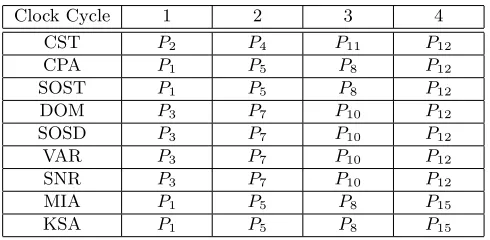
In Table 2, we show the interesting points chosen by different approaches using the 110,000 actual power traces in Set C. From Table 2, we find that our approach chooses different interesting points in the first three clock cycles compared with other approaches.
Table 2.The interesting points chosen by different approaches
Clock Cycle 1 2 3 4
CST P2 P4 P11 P12
CPA P1 P5 P8 P12
SOST P1 P5 P8 P12
DOM P3 P7 P10 P12
SOSD P3 P7 P10 P12
VAR P3 P7 P10 P12
SNR P3 P7 P10 P12
MIA P1 P5 P8 P15
KSA P1 P5 P8 P15
4.2 Group 2
For simplicity, let np and ne respectively denote the number of actual power traces used in the profiling stage and in the extraction stage. In this paper, we use the typical metricsuccess rate [6] as the metric about the classification performance of template attacks.
In order to show the success rates of template attacks based on the inter-esting points chosen by different approaches under different attack scenarios, we conducted 4 groups of experiments. In these groups of experiments, the numbers of actual power traces used in the profiling stage are different. This implies that the level of accuracy of the templates in these groups of experiments are differ-ent. The higher number of actual power traces used in the profiling stage, the more accurate templates will be built. Moreover, in each groups of experiments, we still considered the cases that one can possess different numbers of actual power traces which can be used in the extraction stage.
Specifically speaking, in the 4 groups of experiments, we respectively chose 5,000, 10,000, 15,000, and 20,000 different actual power traces from Set A to build the 256 templates based on the interesting points chosen by different approaches in the profiling stage. Template attacks based on the interesting points chosen by approach A is denoted by the symbol “A-TA”. We tested the success rates of template attacks based on the interesting points chosen by different approaches when one uses ne actual power traces in the extraction stage as follows. We repeated the 9 attacks (CSF-TA, CPA-TA, SOST-TA, DOM-TA, SOSD-TA, SNR-TA, VAR-TA, MIA-TA, and KSA-TA) 1,000 times. For each time, we chose
many times the 9 attacks can successfully recover the correct subkey of the 1st S-box.
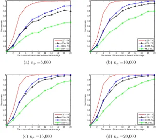
From Table 2, we find that the CPA approach and the SOST approach pro-vide the same result of choosing interesting points. The DOM approach, the SOSD approach, the VAR approach, and the SNR approach provide the same result of choosing interesting points. Moreover, the MIA approach and the KSA approach provide the same result of choosing interesting points. The approaches which provide the same result of choosing interesting points will lead to the same classification performance of template attacks. Therefore, in order to show the success rates more clearly, we only show the success rates of CSF-TA, CPA-TA, DOM-TA, and MIA-TA in Figure 1. The success rates of template attacks based on the interesting points chosen by different approaches whennpequals to 5,000 andne equals to 4, 8, 12, 16,and 20 are shown in Table 3.
0 2 4 6 8 10 12 14 16 18 20 0 0.1 0.2 0.3 0.4 0.5 0.6 0.7 0.8 0.9 1
The number of traces used in the extraction stage
Success rate
CST−TA CPA−TA DOM−TA MIA−TA
(a)np=5,000
0 2 4 6 8 10 12 14 16 18 20 0 0.1 0.2 0.3 0.4 0.5 0.6 0.7 0.8 0.9 1
The number of traces used in the extraction stage
Success rate
CST−TA CPA−TA DOM−TA MIA−TA
(b) np=10,000
0 2 4 6 8 10 12 14 16 18 20 0 0.1 0.2 0.3 0.4 0.5 0.6 0.7 0.8 0.9 1
The number of traces used in the extraction stage
Success rate
CST−TA CPA−TA DOM−TA MIA−TA
(c)np=15,000
0 2 4 6 8 10 12 14 16 18 20 0 0.1 0.2 0.3 0.4 0.5 0.6 0.7 0.8 0.9 1
The number of traces used in the extraction stage
Success rate
CST−TA CPA−TA DOM−TA MIA−TA
(d) np=20,000
Fig. 1.The experiment results
inter-esting points chosen by the previous approaches. For example, whennp= 5,000 andne= 4, the success rate of CST-TA equals to 0.70, while the success rate of DOM-TA equals to 0.32. What’s more, when np = 5,000, CST-TA only need-s 7 actual power traceneed-s in the extraction need-stage to achieve need-succeneed-sneed-s rate higher than 0.9, while DOM-TA needs 20 actual power traces in the extraction stage to achieve success rate higher than 0.9 under the same attack scenario. Therefore, we believe that using our new approach to choose the interesting points can effectively improve the classification performance of template attacks.
Table 3.The success rates of template attacks whennp= 5,000
ne 4 8 12 16 20
CST-TA 0.70 0.94 0.99 1.00 1.00
CPA-TA 0.34 0.58 0.69 0.77 0.79
SOST-TA 0.34 0.58 0.69 0.77 0.79
DOM-TA 0.32 0.63 0.76 0.85 0.90
SOSD-TA 0.32 0.63 0.76 0.85 0.90
VAR-TA 0.32 0.63 0.76 0.85 0.90
SNR-TA 0.32 0.63 0.76 0.85 0.90
MIA-TA 0.19 0.36 0.46 0.53 0.57
KSA-TA 0.19 0.36 0.46 0.53 0.57
5
Conclusion
In this paper, we give a negative answer to the question that whether or not using the previous approaches of choosing interesting points will lead to the best classification performance of template attacks by introduction a new approach with completely different basic principle. Our new approach is based on the important mathematical property of the multivariate Gaussian distribution and exploits the Pearson’s chi-squared test for goodness of fit.
Experiments verified that template attacks based on the interesting points chosen by our new approach will achieve obvious better classification perfor-mance compared with template attacks based on the interesting points chosen by the previous approaches. Moreover, the computational price of our new ap-proach is low and practical. Therefore, our new apap-proach of choosing interesting points can be used in practice to better understand the practical threats of tem-plate attacks. In the future, it is necessary to further verify our new approach in other devices such as ASIC and FPGA.
References
1. Chari, S., Rao, J.R., Rohatgi, P.: Template Attacks. CHES2002, LNCS 2523, pp.
13-28, 2003.
2. Rechberger, C., Oswald, E.: Practical Template Attacks. WISA2004, LNCS 3325,
pp. 440-456, 2004.
3. Archambeau, C., Peeters, E., Standaert, F.-X., Quisquater, J.-J.: Template Attacks
in Principal Subspaces. CHES2006, LNCS 4249, pp. 1-14, 2006.
4. Choudary, O., Kuhn, M.G.: Efficient Template Attacks. CARDIS2013, LNCS 8419,
pp. 253-270, 2013.
5. B¨ar, M., Drexler, H., Pulkus, J.: Improved Template Attacks. COSADE2010, 2010.
6. Standaert, F.-X., Malkin, T.G., Yung, M.: A Unified Framework for the Analysis of
Side-Channel Key Recovery Attacks. EUROCRYPT2009, LNCS 5479, pp. 443-461, 2009.
7. Montminy, D.P., Baldwin, R.O., Temple, M.A., Laspe, E.D.: Improving
cross-device attacks using zero-mean unit-variance mormalization. Journal of Crypto-graphic Engineering, Volume 3, Issue 2, pp. 99-110, June 2013.
8. Oswald, E., Mangard, S.: Template Attacks on Masking—Resistance Is Futile.
CT-RSA2007, LNCS 4377, pp. 243-256, 2007.
9. Standaert, F.-X., Archambeau, C.: Using Subspace-Based Template
Attack-s to Compare and Combine Power and Electromagnetic Information LeakageAttack-s. CHES2008, LNCS 5154, pp. 411-425, 2008.
10. Gierlichs, B., Lemke-Rust, K., Paar, C.: Templates vs. Stochastic Methods A Per-formance Analysis for Side Channel Cryptanalysis. CHES2006, LNCS4249, pp. 15-29, 2006.
11. Mangard, S., Oswald, E., Popp, T.: Power Analysis Attacks: Revealing the Secrets of Smart Cards. Springer 2007.
12. Hanley, N., Tunstall, M., Marnane, W.P.: Unknown Plaintext Template Attacks. WISA2009, LNCS 5932, pp. 148-162, 2009.
13. Jolliffe, I.: “Principal Component Analysis”, John Wiley & Sons, Ltd, 2005. 14. Durvaux, F., Renauld, M., Standaert, F.-X. et al.: Efficient Removal of Random
Delays from Embedded Software Implementations Using Hidden Markov Models. CARDIS2012, LNCS 7771, pp. 123-140, 2013.
15. Coron, J.-S., Kizhvatov, I.: Analysis and Improvement of the Random Delay Coun-termeasure of CHES 2009. CHES2010, LNCS 6225, pp. 95-109, 2010.
16. Mather, L., Oswald, E., Bandenburg, J., W´ojcik, M.: Does My Device Leak
In-formation? An a priori Statistical Power Analysis of Leakage Detection Tests.
ASIACRYPT2013 Part I, LNCS 8269, pp. 486-505, 2013.
17. Gierlichs, B., Batina, L., Tuyls, P., Preneel, B.: Mutual Information Analysis. CHES2008, LNCS 5154, pp. 426-442, 2008.
18. Whitnall, C., Oswald, E., Mather, L.: An Exploration of the Kolmogorov-Smirnov Test as a Competitor to Mutual Information Analysis. CARDIS2011, LNCS 7079, pp. 234-251, 2011.
19. Kocher, P.C.: Timing Attacks on Implementations of Diffie-Hellman, RSA, DSS, and Other Systems. CRYPTO1996, LNCS 1109, pp. 104-113, 1996.
20. Gandolfi, K., Mourtel, C., Olivier, F.: Electromagnetic Analysis: Concrete Results. CHES2001, LNCS 2162, pp. 251-261, 2001.
22. Standaert, F.-X., Koeune, F., Schindler, W.: How to Compare Profiled Side-Channel Attacks? ACNS2009, LNCS 5536, pp. 485-498, 2009.
23. Cover, T.M., Thomas, J.A.: Elements of Information Theory. John Wiley & Sons, Chichester, 2006.
24. Schindler, W., Lemke, K., Paar, C.: A Stochastic Model for Differential Side Chan-nel Cryptanalysis. CHES2005, LNCS 3659, pp. 30-46, 2005.
25. Pearson, K.: On the criterion that a given system of deviations from the probable in the case of a correlated system of variables is such that it can be reasonably supposed to have arisen from random sampling. Philosophical Magazine Series 5 50 (302): pp. 157-175, 1900.
Appendix A: The Proof of Lemma 2
Proof: For simplicity, we only consider the case when N = 2. For the case
N >2, this Lemma holds similarly.
Let (ξ, η) denote a 2 dimensional random vector. The continuous distribution function and the probability density function of the 2 dimensional random vector respectively are F(x, y) and p(x, y). Then, the marginal distribution functions are as follows:
F1(x) =
∫ x
−∞
∫ ∞
−∞
p(u, y)dudy, F2(y) =
∫ ∞
−∞
∫ y
−∞
p(x, u)dxdu.
The marginal density functions are as follows:
p1(x) =
∫ ∞
−∞
p(x, y)dy, p2(y) =
∫ ∞
−∞
p(x, y)dx.
For 2 dimensional multivariate Gaussian distribution, it has that
p(x, y) = 1 2π|C|exp
{
−1
2(x−a, y−b)·C
−1·
(x−a, y−b)T
}
,
where
C=
(
σ12 rσ1σ2
rσ1σ2 σ22
)
and the valuesa, b, σ1, σ2, rare constant,σ1>0, σ2>0,|r|<1. The probability density functionp(x, y) can be rewritten as follows
p(x, y) = 1
2πσ1σ2 √
1−r2exp
{
− 1 2(1−r2)·
[(x−a)2
σ2 1
−2r(x−a)(y−b)
σ1σ2
+(y−b) 2 σ2 2 ]} . Let
x−a σ1
=u,y−b σ2
and it has that
p1(x) =
∫ ∞
−∞
p(x, y)dy
= 1
2πσ1 √
1−r2
∫ ∞
−∞ exp
{
− 1
2(1−r2)·[u
2−2ruv+v2]}dv
=√ 1 2πσ1
e−u2/2
∫ ∞
−∞
1
√
2π(1−r2)·exp
{
−r2u2−2ruv+v2 2(1−r2)
}
dv
=√ 1 2πσ1
e−u2/2
∫ ∞
−∞
1
√
2π(1−r2)e
−(v−ru)2/2(1−r2) dv
=√ 1 2πσ1
e−u2/2=√ 1 2πσ1
e−(x−a)2/2σ12.
Therefore,p1(x) is the probability density function of the normal distribution N(a, σ2
1). Similarly, we can prove that
p2(y) = 1 √
2πσ2
e−(x−b)2/2σ22.