Abstract
GUO, XIANG. Statistical Analysis in Two Stage Randomization Designs in Clinical
Trials. (Under the direction of Dr. Anastasios A. Tsiatis)
Two-stage randomization designs are becoming more common in many clinical trials related to diseases such as cancer and HIV, where an induction therapy is given
followed by a maintenance therapy depending on patients’ response and consent. The main interest is to compare combinations of induction and maintenance therapies and to find the combination leading to the longest average survival time. However, in
practice, the data analysis is typically conducted separately in two stages.
In this Thesis, we tackle the problem based on “treatment policies”. We use the concepts of counting process and risk set as described by Fleming and Harrington
(1991) to find weighted estimating equations whose solution gives an estimator for the cumulative hazard function which, in turn, is used to derive an estimator for the overall survival distribution under a treatment policy with right-censored data. We
call this estimator as the Weighted Risk Set Estimator (WRSE). We show that the WRSE is consistent and asymptotically normally distributed. In addition to survival distribution estimation, we also consider the hypothesis testing problem. Since the
log rank test is the common method for hypothesis testing in survival analysis, we propose a test statistic using an inverse weighted version of the log rank test. We use simulation studies to demonstrate the properties of our method and use data from a
STATISTICAL ANALYSIS IN TWO STAGE RANDOMIZATION
DESIGNS IN CLINICAL TRIALS
by
XIANG GUO
A dissertation submitted to the Graduate Faculty of North Carolina State University
in partial fulfillment of the requirements for the Degree of
Doctor of Philosophy
STATISTICS
Raleigh
2005
APPROVED BY:
Dr. Anastasios A. Tsiatis Dr. Marie Davidian Chair of Advisory Committee
Biography
Xiang Guo was born on December 30th, 1975 to Shengli Guo and Fengming Lei
in Jiangdu, China. He graduated from Jiangdu High School in Jiangdu in 1993. He received a Bachelor of Sciences degree in Probability & Statistics from Peking Univer-sity in Beijing, China in 1997. After working in Ping An insurance company for three
years as a data analyst, he then attended the University of Cincinnati in Cincinnati, Ohio, where he graduated with a Master’s of Sciences degree in Statistics in 2000. He joined the graduate program in the Statistics Department at North Carolina State
Acknowledgements
I would first like to thank my advisor, Dr. Anastasios A. Tsiatis for his guidance,
advice and support throughout my research work. I am also grateful to my committee members, Dr. Marie, Davidian, Dr. John, Monahan and Dr. Daowen Zhang for their valuable suggestions and comments on the revision of the thesis.
I owe thanks to the following people (past and present) in the Statistics Depart-ment of NC State University: Dr. Bibhuti B. Bhattacharyya, Dr. David Dickey, Dr. Leonard Stefanski, Dr. Dennis D. Boos, Dr. Sastry Pantula, Adrian Blue, Terry
Byron and Janice Gaddy.
I couldn’t have accomplished this thesis and this degree without the support from my family. I want to take this time to thank my father, Shengli Guo, for his support,
understanding and encouragement in my pursuit of this degree and to all of my other endeavors in life.
I want to dedicate this work to the loving memory of my mother, Fengming Lei.
Contents
List of Figures vii
List of Tables viii
1 Introduction 1
2 Model Framework and Notation 8
3 Estimation For the Survival Distributions of Treatment policies 12
3.1 Available Estimators . . . 14
3.1.1 Naive Estimator . . . 14
3.1.2 Estimators Based on Inverse Weighting . . . 14
3.2 Weighted Risk Set Estimator . . . 17
3.3 Large-sample Properties . . . 20
3.4 Simulation Study . . . 25
3.5 Application to CALGB Data . . . 28
4.1 Test Statistic for Two-stage Randomization Designs . . . 34
4.1.1 Log Rank Test . . . 34
4.1.2 Weighted Log Rank Test Statistic . . . 35
4.2 Power of the WLR Test . . . 41
4.3 Simulation Study . . . 44
4.3.1 Under Null Hypothesis . . . 45
4.3.2 Under Alternative Hypothesis . . . 51
4.4 Application to CALGB Data . . . 54
5 Discussion 58
Bibliography 60
A Proof: without censoring , WRSE is a member of the class of RAL
estimators proposed by Wahed and Tsiatis (2004) 62
B Proof of proposition 2 67
List of Figures
List of Tables
3.1 Estimates for Survival Distribution . . . 27 3.2 Large Sample Properties of WRSE . . . 28
3.3 Application to CALGB data . . . 30
4.1 The rejection rates, sample means of two tests under the null hypoth-esis and model structure A . . . 46
4.2 Scenarios with different combinations ofαj and βj . . . 48
4.3 The rejection rates, sample means of test statistic under the null hy-pothesis and model structure B . . . 50
4.4 The rejection rates, sample means of WLR test statistic under the alternative hypothesis and model structure B . . . 52 4.5 The rejection rates, sample means of test statistic under the alternative
Chapter 1
Introduction
Some diseases, such as cancers and HIV, have been major threats to human life for
a long time. A lot of effort has been devoted in order to improve the survival time of patients with such diseases. For many of these diseases, it is hard to find a single effective treatment. More and more research is focused on combinations of different
treatments. For example: many breast cancer patients are treated with chemotherapy or hormonal therapy after surgery; patients infected by AIDS now can be treated by “cocktail” therapy, which uses the combination of several drugs. These “combo”
therapies give very significant improvement for patients’ survival time. The AIDs death rate dropped by 47% by 1997 since the implementation of the famous Highly
to 14th place, according to the national Centers for Disease Control and Prevention.
As a result, many clinical trials are studying combinations of several drugs. Two-stage randomization designs is widely used when the combination of two treatments are of interest. In this design, an induction therapy is randomly assigned to a patient
as the patient enters the study. Then, if and only if the patient achieves remission and consent, a maintenance therapy is randomly assigned. One such two-stage random-ized clinical trial, Protocol 8923, was conducted by the Cancer and Leukemia Group
(CALGB) and reported by Stone et al. (1995). It was a double-blind, placebo con-trolled two-stage trial examining the effects of infusions of granulocyte-macrophage colony-stimulating factor (GM-CSF) after initial chemotherapy in 388 elderly
pa-tients with acute myelogenous lukemia (AML). Papa-tients were randomized initially to GM-CSF or placebo following standard chemotherapy. Later, patients who met the criteria for complete remission and consent were offered a second randomization to
one of two intensification treatments.
Because of the randomization, any induction therapy can be assigned to a patient when he/she enters the study. Furthermore, before he/she achieves remission and
consent, we do not know which maintenance therapy will be given or in some cases, there will be no maintenance therapy. Another randomized design is also possible for such two stage study, where the maintenance therapy is pre-specified up front
of induction and maintenance therapies. The advantage of the pre-specified design
is that it makes statistical inference easier. As an example, if we have two induction therapies and two maintenance therapies, we will have a total of four combinations. We can randomly assign patients to these four arms. Then using standard survival
analysis techniques, we can easily find the estimator for the survival distribution and use standard statistical tests for hypothesis testing. But the two-stage randomized design can make more efficient use of the study participants, which makes this design
more efficient than the pre-specified up-front design. But the problem is whether easy-to-implement methods for data analysis under this design can be provided.
In most two-stage randomization design studies, the main interests is to compare
combinations of induction and maintenance therapy and to find the combination lead-ing to the longest average survival time. However, in practice, the data analysis is typ-ically conducted separately in two stages: (i) estimating survival distributions under
different induction therapies using all data while ignoring the maintenance therapies, (ii) estimating survival distributions using data for patients receiving maintenance therapies. These analysis do not directly address the question of finding the best
combination of induction and maintenance therapies.
Th two-stage studies also can be regarded as a special case of the multi-state survival analysis. For each patient entering the study, there can be two states: death
three transition hazards as:
1. λ(u), hazard function from the beginning of the study to death ;
2. µ(t), hazard function from the beginning of the study to response;
3. δ(t, u), hazard function from response to death,
where u is time to death, t is time to response and δ(˙) is a function of both t and u. With the available data, we can find the estimators for three hazard functions. This method can help us to understand the survival distributions in different stages.
But it does not give us an overall view for the distribution under the combinations. And again, the second randomization will add difficulty to the data analysis when we adapt this methodology.
One feasible way to tackle this problem is to use the concept of “treatment pol-icy”. As we mentioned, if we use the pre-specified design, as a patient enters the study, a combination will be assigned. Later if he/she achieves remission/consent,
a maintenance therapy will be given as pre-specified. For this reason, if we are in-terested in the survival probability of patients under a specific arm, we can collect the death or censoring time under that arm and use the Kaplan-Meier estimator to
estimate the survival distribution. Here, the survival time is the overall survival time under a specific arm : treat with an induction therapy followed with a maintenance therapy if and only if the patients achieve remission and consent. It is the time under
remission/consent. It also considers the situation when some patients may not or can
not take the second therapy. In a two-stage randomization design study, a patient assigned to an induction therapy may end up with any one of the maintenance thera-pies or possibly no maintenance therapy. But in the data analysis, we can adapt the
method used for the pre-specified up-front design. We define a treatment policyAjBk
as “treat with a primary therapyAj followed by a maintenance therapyBk if and only
if patients achieve remission and consent to second randomization”. The treatment
policy can be defined in other ways. For example, we also could define a treatment policy AjBk as “treat with a primary therapy Aj followed by a maintenance therapy
Bk if and only if patients achieve remission”. Different definitions of the treatment
policy lead to different data analysis methods. In two stage randomization designs, in order to analyze the data using the second definition of the treatment policy we need to treat the patients who achieve remission but do not consent as missing and
incorporate one more inverse weighting. For simplicity, we will use the first definition. In two-stage randomization designs, the difficulty of statistical inference for a specific treatment policy is that some subjects do not have the treatments consistent
with that treatment policy. For example, consider the estimation or hypothesis testing involving treatment policy A1B1, which is “treating patients with A1 followed with B1 if and only if patient achieve remission and consent to maintenance therapy”. We can divide all subjects assigned to induction therapy A1 into three groups:
to maintenance therapies, which can be called non-responders;
2. patients who achieve remission and consent to maintenance therapies and are
randomly assigned to maintenance therapy B1;
3. patients who achieve remission and consent to maintenance therapies and are randomly assigned to maintenance therapy B2.
Group 1 and 2 are consistent with the treatment policy A1B1, thus their observed death or censoring time can be used as the observed time under the treatment policy. The problem arises in group 3. This group of patients are not consistent with treat-ment policy A1B1. When we conduct statistical inference on treatment policy A1B1, we would not know the survival time for such a policy on patients in group 3.
A naive method is to ignore these subjects and conduct the inference using data from patients who are consistent with A1B1, i.e., subjects in group 1 and 2. As we show in Appendix C, this method is theoretically biased and in most cases underes-timated the survival probability. By considering patients whose treatments are not consistent with a given treatment policy as missing , this problem can be resolved
using inverse weighting method. Recently, estimation of the survival distributions of treatment policies in two-stage randomization designs has been studied by Lunce-ford et al. (2002) (subsequently referred to as LDT) and Wahed and Tsiatis (2004)
of Robins et al. (1994), Wahed and Tsiatis characterized the most efficient
estima-tor for the survival distributions in the case when there is no censoring. Both the LDT and the WT estimators have relatively complicated forms and are difficult to implement in practice. We will propose a new methodology using the concepts of
counting process and risk set as described by Fleming and Harrington (1991) to find weighted estimating equations whose solution gives an estimate for the cumulative hazard function which, in turn, is used to derive an estimator for the overall survival
distribution under a treatment policy with right- censored data. From now on, we call this estimator as the Weighted Risk Set Estimator (WRSE). Since the WRSE is a natural extension of the Aalen-Nelson estimator, it is more intuitive than the
existing estimators. Other advantages of the WRSE include: it is easier to compute and, as we will demonstrate, is more efficient than previously proposed estimators.
On the basis of their estimator for the survival distribution, Lunceford et al (2002)
and Wahed and Tsiatis (2004) used the Wald test to compare treatment policies. Since log rank test is the common method for hypothesis testing in survival analysis, in this thesis, we will also propose a test statistic using a inverse weighted version of the log
Chapter 2
Model Framework and Notation
For concreteness, We will consider the two-stage randomization clinical trials where
patients are initially randomized to one of the induction therapies, say A1 or A2. Then, if eligible and consent is given for maintenance therapies, patients are randomly assigned to one of the maintenance therapies B1 or B2. Our objective is to estimate and compare the survival distributions under the treatment policies AjBk,j, k = 1,2
where AjBk represents the policy “treat with Aj followed byBk if patient is eligible
and consents to maintenance therapy”. As usual, survival time is defined as the time
from initial randomization until death.
As in Lunceford et al. (2002), we conceptualize this problem through potential
outcomes or counterfactuals (Holland, 1991). Assume that each subject i has an associated set of potential outcomes{R1i, R2i, Tj0i, T1Ri, T2Ri, T11∗i, T12∗i, T21∗i, T22∗i}, where
the treatment policies A1Bk, k = 1,2, and similarly for R2i. Tj0i is the survival time
for patientiif he/she is assigned to induction therapyAj and is not eligible or refuses
maintenance therapy. TR
1i is the potential response time that we would observe if
subject i were assigned to one of the treatment policiesA1Bk, k= 1,2, and similarly
for TR
2i. Implicitly, we have made the assumption that potential remission/consent
status is a function only of the induction treatment Aj and is independent of the B
treatment. T∗
jki represent survival time from second randomization to death if patient
i with induction therapy Aj is eligible, willing to receive maintenance therapy and is
assigned to treatmentBk.
With these assumptions, the survival time for patient i, if assigned to treatment policy AjBk, would be Tjki = (1−Ri)Tj0i+Ri(TjiR+Tjki∗ ), j, k = 1,2. Notice that
if Rji = 0, i.e., patient i is not eligible or refuses the maintenance therapy, then
Tj1i =Tj2i =Tj0i.
The set of variables {R1, R2, TR
1 , T2R, T11, T12, T21, T22} is referred as the potential outcomes because they can never be observed at the same time for each patient. These variables represent what potentially would happen under policies.
LetTjk represent the survival time for the population if all patients were assigned
to the treatment policy AjBk. Hence inference on features of these distributions
addresses directly the intent-to-treat question of interest.
Fornpatients that enter our study, letXi denotes the induction treatment
The observed response indicator for theith patient is represented byRi, which equals
1 if the patient achieves remission and consent to further randomization to the main-tenance therapy and 0 otherwise. Rican be related to the potential remission/consent
status byRi =XiR1i+ (1−Xi)R2i. For patients withRi = 1, their response time are
observed and denoted as TR
i . It can also be related to the potential response times
by TR
i =XiT1Ri + (1−Xi)T2Ri. The indicator for B treatment assignment is denoted
byZi, which equals 1 when patient i is assigned with maintenance therapyB1 and 0 with B2. Both TR
i and Zi are only defined for patients achieve remission and consent
to second stage randomization, i.e, Ri=1. If there is no censoring , we would observe
the survival time for i as Ti. Consider patients assigned with induction therapy A1, i.e., Xi = 1, which implies Ri = R1i. Then the observed data can be related to the
potential outcomes as following:
Ti = (1−Ri)T10i+Ri{T1Ri +ZiT11∗i+ (1−Zi)T12∗i}.
The relationship for A2 patients is analogous. Thus the observed data can be repre-sented as a set of i.i.d. random vectors (Xi, Ri, RiTiR, RiZi, Ti), i= 1,· · ·, n.
To account for right censoring, let Ci be the time to censoring. We allow the
censoring distribution to differ by A treatment, i.e. the censoring distributions are Kj(t) = P(Ci < t|Xi = 2− j), j = 1,2. Under these conditions, the observed
data with right censoring can be represented as i.i.d vectors (Ri, RiTiR, RiZi, Ui,∆i),
where ∆i =I(Ti < Ci) and Ui = min(Ti, Ci). For patients who are censored prior to
To derive the estimator for survival distribution and test statistic, we impose two
more assumptions. We assume that Ci is conditionally independent of all other
vari-ables given the induction therapy, i.e.,Ci is independent of (Ri, RiZi, RiTiR, Tj1i, Tj2i)
given Xi =j−1, j = 1,2. We also assume that:
πj =P(Zi = 1|Ri = 1, Xi = 2−j, TjiR, Tj1i, Tj2i, Ci) = P(Zi = 1|Ri = 1, Xi = 2−j),
(2.1) i.e., the second stage randomization is made independently of other potential
out-comes given Ri = 1 and Xj = j −1, j = 1,2. Here πj’s are the probabilities for
patients with induction therapy Aj to be randomized to maintenance therapy B1,
which are defined only when Ri = 1 and are mostly known by design. We allow
Chapter 3
Estimation For the Survival
Distributions of Treatment policies
Since the data from patients who receive different induction treatments are indepen-dent, we will only focus on the data from the patients who receive induction treatment
A1. The analysis of the data from patients who receive induction treatmentA2 is sim-ilar. Thus, from now on, we will index individuals in our study by i = 1,2,· · ·, n, and we will find the estimator for the survival distribution under the two treatment
policies that are associated with the induction treatmentA1, namelyA1B1andA1B2. So in this chapter we will suppress the subscript j on quantities defined in Chapter 2. For example, the probability for patients with remission/consent to be assigned to
B1, π1, will be expressed as π instead.
to the treatment policy A1Bk. Hence inference on features of these distributions
addresses directly the intent-to-treat question of interest. We will estimate the distri-bution for Tk using the observed data from a two-stage randomization design. With
the assumptions in Chapter 2, the survival time for patienti, if assigned to treatment policy A1Bk, would be Tki = (1−R∗i)T0i +Ri∗(TiR +Tki∗), k = 1,2. Tki, k = 1,2.
Tki are also potential outcomes, as only one of them can be observed when patient i
is assigned with a maintenance therapy. Notice that if R∗
i = 0, i.e., patient i is not
eligible or refuses the maintenance therapy, then T1i =T2i =T0i.
Treatment policiesA1B1 andA1B2 are examples of dynamic treatment regimes as defined by Murphy et al. (2001). In a dynamic treatment regime, rules for treatment
assignment are based on time-varying measurements of the study subjects. So, for example, treatment policy A1B1, dictates that patients receive treatment A1 imme-diately and receive B1 if and only if they respond and consent to further treatment. Here the time-varying measurement is the indicator of response and consent.
3.1
Available Estimators
3.1.1
Naive Estimator
We consider estimation of S1k(t) = 1−P(T1k ≤ t)), the survival function for policy
A1Bk. If we have a hypothetical experiment where we could assign A1Bk for all
patients and get the observations for treatment policy A1Bk, then we could use the
standard survival analysis technique to estimate the overall survival distribution. But in a two-stage randomization design, there are some patients who are not consistent
with A1Bk and as a result have no observations forA1Bk. A naive method is to use
the data from those patients who are consistent with that treatment policy. This method is easy to implement, but it is biased. In appendix C, we give a detailed
proof for the biasness of the NAIVE estimator. The NAIVE estimator overestimates the contribution of the non-remitting/consenting to the survival distribution and is theoretically biased. Since in most cases the responders have better survival chance
over the non-remitting/consent. the NAIVE estimator underestimates the overall survival distribution.
3.1.2
Estimators Based on Inverse Weighting
considered for this problem.
To estimate S1k(t) = 1−P(T1k ≤ t) = 1 −F1k(t), ideally, if all subjects were
assigned to A1Bk and there was no censoring, then Ui = Ti = T1ki. Consider A1B1,
a natural estimator for F11(t) is n−1Pni=1I(Ui ≤t). With censoring and
randomiza-tion to maintenance therapy B contingent on remission/consent status, only a subset of the n patients have observed survival time and have actual treatment consistent with A1B1. Lunceford et al. (2002) proposed a class of estimators using two forms of inverse weighting (Robins et al., 1994) to weight the observations from this subset in such a way that, probabilistically, the distribution of the weighted observations mimics that in the ideal case. Let K(t) = P(Ci > t). Every un-censored value
of Ti represents K−1(Ti) individuals, so that, roughly speaking, the response for an
un-censored individual counts for him/herself andK−1(T
i)−1 similar, censored
indi-viduals. Another inverse weight is used for the second randomization to B treatment.
Lunceford et al (2004) define a weight function:
Q1i = 1−Ri+π−1RiZi.
Note that Q1i = 0 if i received B treatment inconsistent with A1B1, i.e., Ri = 1 and
Zi = 0. Q1i = 1 if Ri = 0 and Q1i = π−1 if Ri = 1 and Zi = 1. Thus, when i’s
treatment is consistent with A1B1, Q1i acts as a weight. Non-responders consistent
the weight functionQ1i, Lunceford et al. (2004) proposed a class of estimator for the
survival distribution under treatment policy A1B1:
ˆ
S1LDT(t) = 1−
(
n−1
n
X
i=1
∆i(1−Ri+RiZi/π)I(Ui ≤t)
ˆ K(Ui)
−αn−1
n
X
i=1
∆i(RiZi/π−Ri)
ˆ K(Ui)
)
,
where ˆK(u) is the Kaplan-Meier estimator for the censoring distribution and α is a constant. WithQ2i = 1−Ri+ (1−π)−1Ri(1−Zi), the estimator for survival
distrib-ution under A1B2 is similarly derived. Differentα’s can lead to different estimators. Lunceford et al. (2002) derived the value of α which corresponds to the minimum variance estimator among all LDT estimators. (From now on, the LDT estimator will refer to the minimum variance estimator).
With no censoring and α = 0, the LDT estimator can be expressed as:
ˆ
F1LDT(t) = n−1 n
X
i=1
(1−Ri+RiZi/π)I(Ti ≤t).
The influence function for this estimator can be shown to be equal to :
1−Ri+
RiZi
π
I(Ti ≤t)−F11(t).
Using the semiparametric theory of Robins et al. (1994), Wahed and Tsiatis (2004)
showed that all RAL estimators forF11(t) have an influence function belonging to the class:
1−Ri+
RiZi
π
{I(Ti ≤t)−F11(t)}+Ri(Zi−π/π)f(TiR, Vi), (3.1)
where Vi is a vector of auxiliary covariates collected on individual i prior to second
TR
i and Vi. Wahed and Tsiatis (2004) found the optimal estimators under several
different model assumptions. However, since we are considering censored data here, the results of Wahed and Tsiatis are not relevant.
3.2
Weighted Risk Set Estimator
In developing the Weighted Risk Set Estimator for the survival distribution of a treatment policy, we will rely heavily on the counting process notation as described
by Fleming and Harrington (1991). For the standard one-stage problem, which would be relevant if we were estimating a treatment-specific survival distribution in a one-stage randomized study with censored survival data, the cumulative hazard rate can
be estimated by the Aalen-Nelson estimator given by
ˆ Λ(t) =
Z t
0
dN(u) Y(u) =
X
i∈D(t)
1 Y(Ui)
,
whereD(t) ={i:Ui ≤t,∆i = 1}denotes all the individuals who are observed to fail
before or at time t, and N(u) is the counting process defined as
N(u) =
n
X
i=1
I(Ui ≤u,∆i = 1),
and Y(u) is the at risk process:
Y(u) =
n
X
i=1
I(Ui ≥u).
In our problem, the goal is to estimate the survival distributions ofT1 and T2. We will focus on the estimation of T1, since estimating T2 follows similarly. To motivate the WRSE, consider the hypothetical experiment where all patients were assigned to the treatment policy A1B1, in which case, we could define the potential outcome T1 for all patients and the observed death or censoring timeU1i = min(T1i, Ci). Defining
N1i(u) = I(U1i ≤u,∆i = 1) andY1i(u) = I(U1i ≥u), we could then get an estimator
for the cumulative hazard function as
ˆ
Λ11(t) =
Z t
0
dPn
i=1N1i(u)
Pn
i=1Y1i(u) .
However, in actuality, in a two-stage randomization design, some of the patients who
could have received treatment B1 are instead randomized to receive B2. At a time point t, if a patient have not achieved remission/consent or have achieved remis-sion/consent and is assigned with B1, then the patient is consistent with treatment policyA1B1 and the observed survival time is the survival time underA1B1. But for patients with remission/consent assigned to B2, they are not consistent with A1B1. Thus, from the observed data we cannot observe N1i(u) or Y1i(u) directly for this
part of subjects. Our method is to treat this part as missing and use the inverse weighting method. Since the second randomization, we can use inverse weight on the observations from subjects assigned to B1 and recover the information missed from subjects assigned to B2. To incorporate with the Alan-Nelson estimator, we define a weight function depending on time u,
whereRi(u) = RiI(TiR≤u) andRi,Zi,π,TiR are defined as in Chapter 2. Note that
if at time u, for patient i, a response has not been observed, i.e., Ri(u) = 0. This
patient is still consistent with treatment policy A1B1, thus we assign him/her with weight 1, i.e.,Wi(u) = 1; if patient i have responded and is assigned with maintenance
treatmentB2, i.e.,Ri(u) = 1 andZi = 0, this patient is no longer consistent withA1B1
and get a weight of 0, i.e.,Wi(u) = 0; if patientihave achieved remission/consent and
receives treatment B1 at time u, he/she represents π1 remitting/consenting subjects who could have potentially been assigned toB1, and thus, at timeu, receives a weight ofWi(u) = π1. WithWi∗(u) = 1−Ri(u)+Ri(u)(1−Zi)/(1−π), an analogous argument
may be made for policy A1B2.
The LDT estimators use a weight function Q1i = 1−Ri+RiZi/π, which does not
depend on time u. Consequently, if a patient has a remission, consents to the second randomization, and is randomized to B2, then such a patient receives a weight of 0 at any time u, including time prior to the second randomization. In contrast, Wi(u)
use Ri(u) = RiI(TiR ≤ u) instead of Ri. For subjects assigned with maintenance
therapy B2, if TiR ≤u, i.e., the time point is after the remission, weight of zero will
be assigned. But if TR
i > u, or the assessing time is earlier the response time, a
especially when the response time is long.
With this weight function, we propose an estimator for the cumulative hazard for the survival time under policy A1B1, T1 , as:
ˆ
Λ11(t) =
Z t
0
Pn
i=1Wi(u)dNi(u)
Pn
i=1Wi(u)Yi(u)
, (3.2)
where Ni(u) =I(Ui ≤u,∆i = 1) and Yi(u) =I(Ui ≥ u) are defined on the observed
death or censoring timeUi.
This leads to an estimator for the survival function of T1 as:
ˆ
S1(t) = exp
−
Z t
0
Pn
i=1Wi(u)dNi(u)
Pn
i=1Wi(u)Yi(u)
. (3.3)
Note: When there is no censoring, i.e., Ui =Ti, we can show that the estimator
we derived is a member of the family of RAL estimators proposed by Wahed and Tsiatis (2004). We give a detailed proof in Appendix A.
3.3
Large-sample Properties
In this section, we give a heuristic sketch of steps involved in showing that the WRSE
is consistent and asymptotically normal. We start with two propositions:
Proposition 1 E{Wi(u)Yi(u)}=E{Y1i(u)}.
To prove this proposition, we first show that Wi(u)Yi(u) =Wi(u)Y1i(u), i.e.
{1−Ri(u) +Ri(u)Zi(u)/π}I(Ti ≥u)I(Ci ≥u)
1. If Ri(u) = 1 and Zi = 0, i.e., patient i is assigned to B2, Wi(u) = 0. Thus
equation (3.4) holds and is equal to zero.
2. If Ri(u) = 1 and Zi = 1, i.e., patient i is assigned to B1, then Ti = T1i and
equation (3.4) holds again.
3. IfRi(u) = 0, subjectihas not achieved remission/consent and thus is consistent
with treatment policy A1B1. Therefore Ti =T1i and equation holds.
We complete the proof of proposition 1 as follows:
E{Wi(u)Yi(u)} = E{Wi(u)Y1i(u)}
= E{Wi(u)I(U1i ≥u)}
= E
E{Wi(u)I(U1i ≥u)|Ri, RiTiR, T1i, T2i, Ci}
= E
E{Wi(u)I(T1i ≥u)I(Ci ≥u)|Ri, RiTiR, T1i, T2i, Ci}
= E(I(T1i ≥u)I(Ci ≥u)[1−Ri(u)
+E{Ri(u)Zi/π|Ri, RiTiR, T1i, T2i, Ci}]
(3.5)
= E{I(U1i ≥u)}
= E{Y1i(u)}.
The key to the proof above is that in equation (3.5),
E{Ri(u)Zi/π|Ri, RiTiR, T1i, T2i, Ci}=Ri(u),
Proposition 2 For a deterministic function K(u),
E
Z t
0
K(u)Wi(u){dNi(u)−Yi(u)dΛ11(u)}
= 0.
We give a detailed proof of proposition in appendix B.
With proposition 1 and proposition 2, we will show that the estimator for cu-mulative hazard function is consistent and asymptotically normally distributed. De-fine S1(c)(u) = P(U1i ≥ u). From proposition 1 we know that E{Wi(u)Yi(u)} =
E{Y1i(u)} = S1(c)(u). Then we have a unbiased estimator for S (c)
1 (u) as ˆS (c) 1 (u) = n−1Pn
i=1Wi(u)Yi(u). Using the large sample theory, we deduce that
n
ˆ
S1(c)(u)−S1(c)(u)o converges in probability to 0 uniformly in u. By adding and subtracting common terms, {Λ11(t)ˆ −Λ11(t)} can be expressed as:
ˆ
Λ11(t)−Λ11(t) = n−1
n
X
i=1
Z t
0
Wi(u){dNi(u)−Yi(u)dΛ11(u)}
S1(c)(u) (3.6) +n−1
n X i=1 Z t 0 n
1/Sˆ1(c)(u)−1/S1(c)(u)oWi(u){dNi(u)−Yi(u)dΛ11(u)}. (3.7) To show consistency, we first notice that
E
" Z t
0
Wi(u){dNi(u)−Yi(u)dΛ11(u)}
S1(c)(u)
#
= 0.
This follows from proposition 2 by taking K(u) = 1/S1(c)(u). Since expression (3.6) is the sample average of mean zero i.i.d random variables, it converges in probability
probability to zero. It follows from the inequality: Z t 0 n
1/Sˆ1(c)(u)−1/S1(c)(u)on−1
n
X
i=1
Wi(u){dNi(u)−Yi(u)dΛ11(u)}
≤sup
u≤t
1/Sˆ
(c)
1 (u)−1/S (c) 1 (u) (3.8) × (
n−1
n
X
i=1
Z t
0
Wi(u)dNi(u) +n−1 n
X
i=1
Z t
0
Wi(u)Yi(u)dΛ11(u)
)
. (3.9)
Expression (3.8) will converges to zero as long as S1(c)(t) > 0. The first term of expression (3.9) is bounded by 1/π and the second term converges in probability
to E[Rt
0 Wi(u)Yi(u)dΛ11(u)]. Collecting these developments demonstrates that (3.7) converges in probability to zero.
Now we argue that n1/2{Λ11(t)ˆ −Λ11(t)}, which equals n1/2{(3.6) + (3.7)}, con-verges in distribution to a normal with mean zero. Since (3.6) is made up of a sum of i.i.d mean zero random variables, a simple consequence of the central limit theorem leads to the asymptotic normality of n1/2{(3.6)}. To complete the proof, we need to show that n1/2{(3.7)} converges in probability to zero. Expression (3.7) times n1/2 can be written as:
Z t
0
n1/2n1/Sˆ1(c)(u)−1/S1(c)(u)on−1
n
X
i=1
Wi(u){dNi(u)−Yi(u)dΛ11(u)}. (3.10)
Define
ˆ
Hn(t) = n−1
Z t
0
n
X
i=1
Wi(u){dNi(u)−Yi(u)dΛ11(u)},
E[Rt
in t. Expression (3.10) may be rewritten as:
Z t
0
n1/2n1/Sˆ1(c)(u)−1/S1(c)(u)odHˆn(t). (3.11)
Under suitable regularity conditions, n1/2n1/S(c)
1 (u)−1/S (c) 1 (u)
o
will converge to a Gaussian process with continuous paths and by using method similar to Breslow and
Crowley (1974) or Tsiatis (1981), (3.11) will converge in probability to zero. Hence we have,
n1/2{Λ11(t)ˆ −Λ11(t)}=n−1/2
n
X
i=1
Z t
0
Wi(u){dNi(u)−Yi(u)dΛ11(u)}
S1(c)(u) +op(1), where op(1) is a term that converges in probability to zero.
Thus, ˆΛ11(t) is a consistent estimator of Λ11(t) and n1/2{Λ11(t)ˆ − Λ11(t)} ∼ N(0, σ2), where
σ2 =E
"
Z t
0
Wi(u){dNi(u)−Yi(u)dΛ11(u)}
S1(c)(u)
#2
. Replacing dΛ11(u) and S1(c)(u) by consistent estimators dΛ11(u) =\ Pn
i=1Wi(u)dNi(u) P
n
i=1Wi(u)Yi(u) and ˆS1(c)(u) =n−1Pn
i=1Wi(u)Yi(u), we can get a consistent estimator for σ2 as: ˆ
σ2 =n−1
n X i=1 Z t 0
Wi(u)
h
dNi(u)−Yi(u)
nP n
i=1Wi(u)dNi(u) Pn
i=1Wi(u)Yi(u)
oi
n−1Pn
i=1Wi(u)Yi(u)
2 ,
and a consistent estimator for V AR(ˆΛ11(y)) as n−1σˆ2. By the delta method, ˆS1(t) is also consistent and we obtain a consistent variance estimator for ˆS1(t) as :
[
3.4
Simulation Study
In this section, we conduct several simulation studies to investigate the large sample properties of the WRSE and compare the WRSE with the existing NAIVE estimator and LDT estimator for right-censored data. For simplicity, we only simulate data for
“A1” patients.
We take Ri, the response and consent indicator, to be a Bernoulli with P(Ri =
1) =θ. Two different values 0.5 and 0.8 forθ are used in the simulations. IfRi equals
zero, we then generate a survival time T0i, which follows an exponential distribution
with mean 182.5 days. T0i is the survival time of the patients who do not respond or
do not consent for maintenance therapies, and it is generated only if Ri = 0. When
Ri = 1, a time to response TiR is generated following a exponential distribution with
mean 365 days. If Ri = 1, we also generate a treatment B assignment indicator Zi
from Bernoulli(0.5) distribution. If Zi = 1, a survival timeT1∗i will be generated from
an exponential distribution with mean 365 days and if Zi = 0, another survival time
T∗
2i will be generated from an exponential distribution with mean 547.5 days. T1∗i is
the survival time from remission/consent to death ifB1is assigned as the maintenance treatment and T∗
2i is the survival time from remission/consent to death when B2 is
assigned. The observed survival time for the ith individual thus can be defined as
Ti = (1−Ri)T0i+Ri{TiR+ZiT1∗i+ (1−Zi)T2∗i}.
We set the censoring time Ci to be uniformly distributed between zero and 3.5 years,
censoring time to be Ui =min(Ti, Ci). For simplicity, we only calculate the estimate
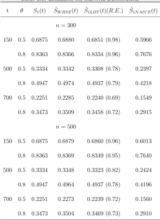
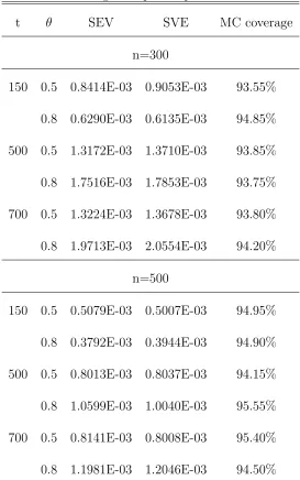
for S1(t) =P(T1 > t), which is the survival distribution for treatment policy A1B1. For each of 2000 Monte Carlo data sets,S1(t) is estimated using (3.3) respectively at t = 150, 500 and 700 days. The variance of ˆS1(t) is also estimated using (3.12). For each estimand, the 95% Wald confidence interval is constructed as the estimator plus or minus the appropriate standard error from (3.12) times 1.96. Both NAIVE estimates and LDT estimates are also considered. To compare the WRSE and the
LTD estimators, which are both unbiased, we use the relative efficiency defined as following:
R.E. = sample variance of WRSE estimator sample variance of the LDT estimator,
i.e., the ratio between the sample variance of WRSE and the sample variance of LTD. Table 3.1 presents the estimates of the survival distribution under treatment policy A1B1 using the WRSE, LTD and NAIVE method along with the relative efficiency between WRSE and LTD. Table 3.2 presents some large sample properties of our estimator. We give sample average of the estimated variance (SEV) and sample variance of the estimator (SVE) for the survival function.
From Table 3.1, we find that the WRSE and the LDT estimator both are unbiased and there is significant bias for the NAIVE estimator. In term of the relative efficiency, the WRSE is more efficient than the LDT estimator, with the biggest gains in the
Table 3.1: Estimates for Survival Distribution
t θ S1(t) SˆW RSE(t) S1ˆLDT(t)(R.E.) S1ˆN AIV E(t)
n = 300
150 0.5 0.6875 0.6880 0.6851 (0.98) 0.5966 0.8 0.8363 0.8366 0.8334 (0.96) 0.7676 500 0.5 0.3334 0.3342 0.3308 (0.78) 0.2397
0.8 0.4947 0.4974 0.4937 (0.79) 0.4218 700 0.5 0.2251 0.2285 0.2240 (0.69) 0.1549 0.8 0.3473 0.3509 0.3458 (0.72) 0.2915
n = 500
150 0.5 0.6875 0.6879 0.6860 (0.96) 0.6013 0.8 0.8363 0.8369 0.8349 (0.95) 0.7640
500 0.5 0.3334 0.3348 0.3323 (0.82) 0.2424 0.8 0.4947 0.4964 0.4937 (0.78) 0.4196 700 0.5 0.2251 0.2273 0.2239 (0.72) 0.1560
0.8 0.3473 0.3504 0.3469 (0.73) 0.2910
Table 3.2: Large Sample Properties of WRSE
t θ SEV SVE MC coverage
n=300
150 0.5 0.8414E-03 0.9053E-03 93.55% 0.8 0.6290E-03 0.6135E-03 94.85% 500 0.5 1.3172E-03 1.3710E-03 93.85%
0.8 1.7516E-03 1.7853E-03 93.75% 700 0.5 1.3224E-03 1.3678E-03 93.80% 0.8 1.9713E-03 2.0554E-03 94.20%
n=500
150 0.5 0.5079E-03 0.5007E-03 94.95%
0.8 0.3792E-03 0.3944E-03 94.90% 500 0.5 0.8013E-03 0.8037E-03 94.15% 0.8 1.0599E-03 1.0040E-03 95.55%
700 0.5 0.8141E-03 0.8008E-03 95.40% 0.8 1.1981E-03 1.2046E-03 94.50%
3.5
Application to CALGB Data
We demonstrate how to apply the proposed methodology to a two-stage
two years), the data did not contain appreciable censoring. In order to illustrate the
performance of various estimators with censored survival data, we artificially censored the data by restricting the follow-up period to 2.5 years after the first enrollment. By doing so, the censoring rate is approximately 27%. Of this data set, 79 out of 193
patients in the GM-CSF group and 90 out of 195 in the placebo group achieved remis-sion and consented to further randomization to intensification therapies; and of these, 37 GM-CSF and 45 placebo patients were randomized to intensification therapy I and
the rest to intensification therapy II.
Our method was used to estimate the survival distributions for all four com-binations. The estimates for the four treatment policies do not show appreciable
differences, consistent with the reported interpretation of CALGB 8923 in Stone et al. (1995).
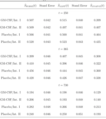
In Table 3.3, we present the estimates of the survival probabilities for each of the
four treatment policies using NAIVE estimator, LDT estimator and WRSE, respec-tively, at times 250, 365 and 730 days. The LDT and our estimator give similar esti-mates while the NAIVE estimator gives significantly smaller estimate. The NAIVE
estimator is theoretically biased and the result is underestimated. From Table 3.3, we also notice that at 250 days and 365 days the variance estimates of the LDT and our method are very similar. At 730 days, when the estimation is at the end of the
Table 3.3: Application to CALGB data ˆ
SW RSE(t) Stand Error S1ˆLDT(t) Stand Error S1ˆN AIV E(t)
t= 250
GM-CSF/Int. I 0.507 0.042 0.515 0.040 0.399 GM-CSF/Int. II 0.509 0.042 0.497 0.041 0.407
Placebo/Int. I 0.566 0.041 0.560 0.041 0.464 Placebo/Int. II 0.520 0.043 0.523 0.043 0.435
t= 365
GM-CSF/Int. I 0.399 0.046 0.407 0.045 0.308 GM-CSF/Int. II 0.410 0.045 0.396 0.046 0.322 Placebo/Int. I 0.456 0.046 0.444 0.045 0.360
Placebo/Int. II 0.420 0.046 0.426 0.047 0.338 t= 730
GM-CSF/Int. I 0.194 0.046 0.198 0.046 0.129
GM-CSF/Int. II 0.206 0.045 0.193 0.048 0.140 Placebo/Int. I 0.282 0.048 0.266 0.048 0.213 Placebo/Int. II 0.248 0.046 0.250 0.051 0.193
From this application, we do not find much improvement by using the WRSE. As we have pointed out, the WRSE is more efficient than the LDT estimator because it
zero in the extreme case, the LDT estimator is equivalent to the WRSE. Since, in this
study, the response to the induction treatment, if it occurs, occurs early in the study as compared to the survival times (the mean survival time is more than 200 days while the mean response time is about 35 days), we would not expect appreciable
Chapter 4
Hypothesis Testing for Treatment
policies
In Chapter 3, we focused on the estimation of the overall survival distribution of treatment policies in two-stage randomization designs. We treated this as a missing
data problem and used the inverse weighting method together with the Aalan-Nelson estimator to derive the WRSE estimator for the cumulative hazard function and the survival function. A natural follow-up is: how we can compare the survival
distributions of two different treatment policies? In the paper of Lunceford et al. (2002) and Wahed and Tsiatis (2004), they both used the Wald test based on the difference of the estimated survival distribution between treatments at specific points
analysis is the log rank test, in this chapter we will derive a hypothesis testing method
based on the standard log rank test.
We will only focus on the hypothesis testing problem comparing the survival distributions of treatment policies A1B1 and A2B1 . The method for comparing other pairs of treatment policies are analogous. Since we will compare two different treatment policies, we will again use the index j which is suppressed in Chapter 3 when we derived the estimator for the survival distribution under one treatment
policy. Denote the survival distribution asS(x, j) =P r(Uj1 > x|Xi =j−1), j = 1,2.
The null hypothesis we want to test is that there is no difference between treatment policiesA1B1andA2B1 in term of overall survival distribution, i.e.,S(x,1) =S(x,2). Our objective is to compare the survival time under treatment policies A1B1 and A2B1, i.e compare the distributions of T11 and T21. Tj1 represents survival time for the population if all patients with induction therapy Aj were assigned to treatment
policy AjB1. In a two-stage randomization design study, patients with induction
4.1
Test Statistic for Two-stage Randomization
De-signs
4.1.1
Log Rank Test
We motivate our test statistic as the natural analog of the standard two-sample log rank test which compares the distributions of the survival time from two independent samples. Considering a hypothetical experiment, we could observe both U11 and U21 which denote the observed death or censoring time for treatment policies A1B1 and A2B1 and could be defined as:
Uj1i = min(Tj1i, Ci), j = 1,2,
where Ci is the censoring time. Assuming that all deaths among n patients happen
at d time points. The log rank test therefore has the following form:
d
X
i=1
(d11i−e11ˆ i),
where the summation is made at each death time point i= 1, . . . , d, dj1i is the total
number of deaths from treatment policies AjB1 at the ith death time point and ˆej1i
is the expected number of deaths from treatment policiesAjB1 at the ith death time
point and can be expressed as
diY11i
Y11i+Y21i
.
Yj1i represents the total number at risk from groupAjB1 at theith death time point
Using counting process representation, we can express the test as:
Z
dN11(u)Y21(u)−dN21(u)Y11(u) Y11(u) +Y21(u)
=
Z Y11(u)Y21(u)
Y11(u) +Y21(u)
dN11(u) Y11(u) −
dN21(u) Y21(u)
, (4.1)
where N11i(u) = I(U11i ≤ u,∆i = 1), N21i(u) = I(U21i ≤ u,∆i = 1), Y11i(u) =
I(U11i ≥ u) and Y21i(u) = I(U21i ≥ u). Under the null hypothesis, the asymptotic
distribution of n−1/2(4.1) is normally distributed with mean zero.
In a two-stage randomization design study, U11, U21 are not observable for some patients. A NAIVE method is to use the log rank test on the data from subjects consistent with the treatment policies that we are interested in, while ignoring the
subjects who do not have the observed time for U11 or U21. As we have mentioned in Chapter 3, this method does not properly reflect the ratio between subjects with remission/consent and subjects without remission/consent and therefore causes bias.
In the rest of this chapter, we will derive a test statistic which uses the inverse weighting method with the observed data that mimics the log rank test given by (4.1) in the hypothetical experiment. It is unbiased and easy to implement.
4.1.2
Weighted Log Rank Test Statistic
Due to the second randomization, we can not observe the survival time under
treat-ment policy AjB1 for some patients. Simply ignoring this data can lead to biased
inverse weighting methods to derive a weighted log-rank test statistic for comparing
the overall survival distributions of treatment policies.
The processes N11i, N21i, Y11i and Y21i in expression (4.1) are defined on the
po-tential outcomes U11i and U21i. To make inference based on the observed data, we
define N1i(u) = I(Ui ≤ u,∆i = 1, Xi = 1), N2i(u) = I(Ui ≤ u,∆i = 1, Xi = 0),
Y1i(u) = I(Ui ≥ u, Xi = 1) and Y2i(u) = I(Ui ≥ u, Xi = 0). We also define two
weight functions respectively for two groups with treatment policies AjB1, j = 1,2, as follows:
Wji(u) = 1−Ri(u) +Ri(u)Zi/πj, j = 1,2, (4.2)
whereRi(u) = RiI(TiR≤u) and πj is the probability for a remission/consent patient
to be assigned to maintenance therapy Bj.
Wji(u) are functions depending on time u. They assign different weights to each
subject according to their status at each time point u. For example, if subject i is assigned toA1, at any timeu, the weight functionW1i(u) will give weight according to
his/her response status and B treatment assignment. If, at a time pointu,Ri(u) = 0,
i.e., i does not achieve remission or does not consent to maintenance therapy, i is consistent with treatment policy A1B1 and thusW1i(u) = 1; ifRi(u) = 1 andZi = 0,
which means thatiachieve remission and is assigned to maintenance groupB2, subject iis no longer consistent with treatment policyA1B1 at this time point and the weight function results in zero ,W1i(u) = 0; ifRi(u) = 1 andZi = 1, patienti, who achieves
treatment policy A1B1 and gets a weight of 1/π1.
The overall survival function under a treatment policy is actually a mixture dis-tribution of the survival disdis-tribution of the remission/consent subjects (who also can be referred to as responders) and that of the non-responders. Another factor which
determines the mixture distribution is the ratio of responders and non-responders. The naive methods for estimation and hypothesis testing in a two-stage randomiza-tion study lead to biased results because they use the wrong ratio and overestimate
the distribution of the non-responders by simply ignoring the patients assigned with treatments not consistent with the policies of interest.
The test statistic for the log rank test is determined by the number at risk and
the number of deaths at each time point when a death occurs. As we have mentioned above, in a two-stage randomization design study, we can not observe the processes needed to calculate the log rank test (4.1) for all the patients. We treat this problem
as a missing data problem and consider the inverse weighting method using the weight functions defined above. Thus substituting the weight function, defined in (4.2), into the log rank test, we derive an inverse weighted version of the log rank test for
comparing treatment policies in two-stage randomization designs as follows:
Zn =
Z Pn
i=1W1i(u)Y1i(u)Pni=1W2i(u)Y2i(u)
Pn
i=1W1i(u)Y1i(u) +
Pn
i=1W2i(u)Y2i(u)
×
Pn
i=1W1i(u)dN1i(u)
Pn
i=1W1i(u)Y1i(u) −
Pn
i=1W2i(u)dN2i(u)
Pn
i=1W2i(u)Y2i(u)
. (4.3)
of zero to subjects who are not consistent with the treatment policies at time u, i.e., subjects achieve remission/consent but assigned to another maintenance therapy by randomization. With a weight of zero, such patients are excluded from the risk set. This agrees with our intuition to ignore those patients who are not consistent with
the policies. However, by doing so, we have changed the ratio between the respon-ders and non-responrespon-ders. With the second randomization, every subject assigned with maintenance therapy B1 can represents 1/πj subjects who could potentially be
assigned to treatment policy AjB1. So we assign a weight of 1/πj to subjects who
achieve remission/consent and are assigned to maintenance therapy B1. With the weight function , we can assure that we use the right ratio and mimic the two sample
log-rank test in the hypothetical experiment.
Next we will show the asymptotic normality ofn−1/2Z
n under the null hypothesis
λ11(u) =λ21(u) = λ(u).
From Chapter 3, we have two propositions:
E{Wji(u)Yji(u)}=E{Yj1i(u)},
and for a deterministic function D(u),
E
Z t
0
D(u)Wji(u){dN1i(u)−Y1i(u)dΛ11(u)}
= 0.
Sj(c)(u). Defining
K(u) = S (c) 2 (u) S1(c)(u) +S2(c)(u) and
ˆ K(u) =
Pn
i=1W2i(u)Y2i(u)
Pn
i=1W2i(u)Y2i(u) +Pni=1W2i(u)Y2i(u)
,
we obtain that ˆK(u) converges in probability to K(u) as long as K(u) > 0. This assumption is valid in most cases since in most clinical trials the follow-up time is limited and we can define an upper bound “τ” for the survival time such thatS(τ)≥ǫ for ǫ > 0. Accordingly, the upper bound for the integral in (4.3) should also be τ. For abbreviation, we will suppress it in the rest of the thesis.
Now notice that Zn can be expressed as:
Z ˆ
Y11(u) ˆY21(u) ˆ
Y11(u) + ˆY21(u)
( Pn
i=1W1i(u)dN1i(u) ˆ
Y11(u)
−
Pn
i=1W2i(u)dN2i(u) ˆ
Y21(u)
)
=
Z ˆ
Y11(u) ˆY21(u) ˆ
Y11(u) + ˆY21(u)
( Pn
i=1W1i(u)dN1i(u) ˆ
Y11(u) −λ(u)du
)
−
Z ˆ
Y11(u) ˆY21(u) ˆ
Y11(u) + ˆY21(u)
( Pn
i=1W2i(u)dN2i(u)
ˆ
Y21(u) −λ(u)du
)
=
Z Y11(u) ˆˆ Y21(u)
ˆ
Y11(u) + ˆY21(u)
Pn
i=1W1i(u){dN1i(u)−λ(u)Y1i(u)du} ˆ
Y11(u)
−
Z ˆ
Y11(u) ˆY21(u) ˆ
Y11(u) + ˆY21(u)
Pn
i=1W2i(u){dN2i(u)−λ(u)Y2i(u)du}
ˆ Y21(u) = Z ˆ Y21(u) ˆ
Y11(u) + ˆY21(u)
n
X
i=1
W1i(u){dN1i(u)−λ(u)Y1i(u)du}
−
Z ˆ
Y11(u) ˆ
Y11(u) + ˆY21(u)
n
X
i=1
W2i(u){dN2i(u)−λ(u)Y2i(u)du}
= Z ˆ K(u) n X i=1
−
Z
{1−K(u)ˆ }
n
X
i=1
W2i(u){dN2i(u)−λ(u)Y2i(u)du}.
Thus,
n−1/2Zn = n−1/2
Z ˆ K(u) n X i=1
W1i(u){dN1i(u)−λ(u)Y1i(u)du}
−n−1/2
Z
{1−K(u)ˆ }
n
X
i=1
W2i(u){dN2i(u)−λ(u)Y2i(u)du}
= n−1/2
Z
K(u)
n
X
i=1
W1i(u){dN1i(u)−λ(u)Y1i(u)du} (4.4)
−n−1/2
Z
{1−K(u)}
n
X
i=1
W2i(u){dN2i(u)−λ(u)Y2i(u)du} (4.5)
+n−1/2
Z
{K(u)ˆ −K(u)}
n
X
i=1
W1i(u){dN1i(u)−λ(u)Y1i(u)du}(4.6)
+n−1/2
Z
{K(u)ˆ −K(u)}
n
X
i=1
W2i(u){dN2i(u)−λ(u)Y2i(u)du}(4.7)
Using method similar to Chapter 3, We can show that (4.6) and (4.7) converge to
zero. From Proposition 2, we know that
E[ Z K(u) n X i=1
W1i(u){dN1i(u)−λ(u)Y1i(u)du}] = 0
and
E[
Z
{1−K(u)}
n
X
i=1
W2i(u){dN2i(u)−λ(u)Y2i(u)du}] = 0
by taking D(u) = K(u) and D(u) = 1− K(u). Then by central limit theorem, (4.4) and (4.5) are asymptotically normally distributed with mean zero and their asymptotic variance are respectively :
E " Z K(u) n X i=1
W1i(u){dN1i(u)−λ(u)Y1i(u)du}
#2
and E " Z
{1−K(u)}
n
X
i=1
W2i(u){dN2i(u)−λ(u)Y2i(u)du}
#2
(4.9)
Because of the independence of (4.4) and (4.5), n−1/2Z
n converges in distribution
to a normal distribution with mean zero and variance σ2 = {(4.8) + (4.9)}. The asymptotic variance can be estimated as:
ˆ
σ2 = 1/n
n
X
i=1
" Z
{K(u)ˆ }
n
X
i=1
W1i(u){dN1i(u)−ˆλ(u)Y1i(u)du}
#2 +1/n n X i=1 " Z
{1−Kˆ(u)}
n
X
i=1
W2i(u){dN2i(u)−λ(u)Y2ˆ i(u)du}
#2
,
where ˆλ(u) = dN1i(u)+dN2i(u)
Y1i(u)+Y2i(u) is the pooled estimator for λ(u), whose true value is not available to us, assuming null hypothesis is true. Therefore we propose a test statistic
for hypothesisλ11(u) =λ21(u) =λ(u) as:
n−1/2Z
n
{σˆ2}1/2 (4.10)
4.2
Power of the WLR Test
In this section we will consider the power that the WLR test has to detect alternatives away from null hypothesis. Since in the asymptotic study of hypothesis testing the test has power converging to one to detect fixed alternatives as the sample sizes
Consider the null hypothesis and alternative hypotheses as a sequence in n:
H0n:λ21n(u) = λ11(u)
H1n:λ21n(u) = λ11(u) exp{BnΘ(u)},
where Θ(u) is a known function of u and Bn converges to zero at the rate of n−1/2,
that is √nBn →Γ6= 0.
Under the alternative hypotheses,
n−1/2Zn = n−1/2
Z ˆ K(u) n X i=1
W1i(u)dN1i(u)−n−1/2
Z
{1−K(u)ˆ }
n
X
i=1
W2i(u)dN2i(u)
= n−1/2
Z ˆ K(u) n X i=1
W1i(u){dN1i(u)−λ11(u)Y1i(u)du} (4.11)
− n−1/2
Z
{1−K(u)ˆ }
n
X
i=1
W2i(u){dN2i(u)−λ11(u) exp{BnΘ(u)}Y2i(u)du(4.12)}
+ n−1/2
Z Y11(u) ˆˆ Y21(u)
ˆ
Y11(u) + ˆY21(u)
λ11(u) [1−exp{BnΘ(u)}]du. (4.13)
Using a taylor series expansion
exp{BnΘ(u)}= 1 +BnΘ(u) +O(n−1).
Thus (4.13) can be expressed as
n−1/2
Z Y11(u) ˆˆ Y21(u)
ˆ
Y11(u) + ˆY21(u)
λ11(u) [1−exp{BnΘ(u)}]du
=n−1/2
Z
ˆ
Y11(u) ˆK(u)λ11(u){−BnΘ(u) +O(n−1)}du
=n−1/2
Z ˆ K(u) n X i=1
W1i(u)Y1i(u)λ11(u){−BnΘ(u)}du
+n−1/2
Z
ˆ
=−
Z
ˆ
K(u)n−1
n
X
i=1
W1i(u)Y1i(u)n1/2BnΘ(u)λ11(u)du (4.14)
+
Z
ˆ
K(u)n−1
n
X
i=1
W1i(u)Y1i(u)O(n−1/2)λ11(u)du (4.15)
In expression (4.15), we have ˆK(u) → K(u), n−1Pn
i=1W1i(u)Y1i(u) → S (c)
1 (u) and O(n−1/2)→0. As a result, (4.15) converges to zero. (4.14) converges to
β =−Γ
Z
K(u)S1(c)(u)Θ(u)λ11(u)du, which is a direct result of n1/2B
n converging to Γ.
Using method similar to Chapter 3, we can show that (4.11) converges to a normal distribution with mean zero and variance as expression (4.8). We can also show that
(4.12) converges to a normal distribution with mean zero and variance as expression (4.9). Since (4.11) and (4.12) are independent, we conclude that, under alternative hypotheses, the numerator of the test statistic converges to a normal distribution
with mean β and variance σ2 = (4.8) + (4.9). For the sequence of alternatives, H1
n,
as n gets larger, H1n gets closer to H0. Using the theory of contiguity developed by
LeCam, we can show that ˆσ2 converges toσ2 under the alternative hypothesis. Thus under the alternative, the test statistic converges in distribution to a normal with mean β/σ and variance 1.
To find an explicit expression for the asymptotic power, we need an explicit form
To illustrate the power calculation, during the above derivation, we assume
propor-tional hazards between two treatment policies. This assumption makes the derivation easier but may not hold in practice due to the complicated structure of the survival time in terms of response and length of response. Thus, it is difficult to find a general
scenario for the asymptotic power. One realistic way to investigate the power is to use simulations once we make assumptions about the distribution of the overall survival time. In the next section we will investigate the power under two model settings.
4.3
Simulation Study
The overall survival distribution is determined by several factors, such as the
dis-tributions of responders and non-responders, the ratio between responders and the non-responders, the distribution of the response time TR and the distribution of the
time for second stage for the responders. There are different ways to construct the
overall distribution. The behavior of our weighted log rank (WLR) test statistic and the naive log rank (NLR) test statistic may both be affected by the model set-tings. In the rest of this chapter we will investigate the performance of the WLR and
4.3.1
Under Null Hypothesis
Assuming the null hypothesis is correct, the overall survival distribution forA1B1 and A2B1 are the same. In the first study, we will assume that subjects in two treatment policy groups have exactly the same distribution.
For each subject, define Xi as the induction therapy indicator, which follows
a Bernoulli(0.5) distribution. Also define Ri as the response indicator, which also
follows a Bernoulli(0.5) distribution. If Ri = 0, we assign a survival time Ti from
an exponential distribution with mean 1.5 years. For subjects with Ri = 1, TiR is
generated from an exponential distribution with mean 0.5 year and Zi is generated
from Bernoulli(0.5) independently. TR
i is the response time and Ziis the maintenance
therapy assignment indicator defined as before. For subjects with Zi = 1, the time
from response to deathT Si is generated from an exponential distribution with mean
2.5 years and with mean 1.5 years if Zi = 0. From now on we refer this model
structure as model A. We use the WLR test and NLR test on 2000 Monte Carlo data
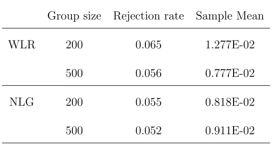
sets, the rejection rates and sample means are summarized respectively for WLR and NLR in table 4.1.
From the result we can find that the WLR test gives rejection rates close to
the nominal value. In Appendix C, we show that the NAIVE method gives biased estimates of the treatment-specific survival distribution ifP(Ti < t|Ri = 1)6=P(Ti <
t|Ri = 0). Thus under this model structure the estimated hazard rates are incorrect
Table 4.1: The rejection rates, sample means of two tests under the null hypothesis and model structure A
Group size Rejection rate Sample Mean
WLR 200 0.065 1.277E-02
500 0.056 0.777E-02
NLG 200 0.055 0.818E-02
500 0.052 0.911E-02
rates is still zero. This explains why the NLR test gives type I errors very close to the nominal value.
Does the NLR work well under every model structure? The answer is no. In real
life, a drug can affect the response rate but not the overall survival. In the second study, we will consider the situation where the subjects in two treatment policy groups have same overall survival distribution, while their response rates are correlated with
the overall survival time and different between two groups. We will see that under this model structure the NLR test is biased and gives inflated type I errors.
Assume the overall survival time for two treatment policy groups A1B1 andA2B1 have the same distribution. A overall survival time Ti is generated for each subjecti
from a exponential distribution with mean 2 years. For each subjecti, the induction therapy assignment indicatorXi is generated from a Bernoulli distribution with
distribution, but the probability is a function of Ti as following:
p= exp(αj+βjTi) 1 + exp(αj +βjTi)
, (4.16)
where j=1 if subject iis assigned to induction therapy A1 and 2 forA2. By doing so, we make the response rate different between two treatment policy groups through a function of the overall survival time. Since P(Ri = 1|Ti) = gj(Ti), we can conclude
that P(Ti < t|Ri = 1) 6= P(Ti < t|Ri = 0), which induces bias when we use the
naive method (see appendix C for the proof that if the equality holds, the naive method is also unbiased). If Ri = 1, since subject i is a responder, an indicator for
maintenance therapy assignment Zi is generated from Bernoulli(0.5). At the same
time we generate a response time TR
i for subject i, which is uniformly distributed
in (0, Ti). Define T Si = Ti − TIR, which is the time from second randomization
until death (we assume that there is no time delay between the response and second
randomization for simplicity). For patients with Zi = 0 or the patients assigned to
B2, they are not consistent with the treatment policies of interest. To make their overall distribution different with patients assigned to B1, we generate T Si from an
exponential distribution with mean two years and redefine Ti =TiR+T Si if Zi = 1.
Thus, for patients consistent with treatment policies AjB1, j = 1,2, they have the
same overall distribution from exp(2). But their response indicators are related to
the overall survival time through a function gj(Ti), j = 1,2 and are different for two
Table 4.2: Scenarios with different combinations ofαj and βj
Scenario 1 Scenario 2 Scenario 3 Scenario 4
α1 -3.0 -3.0 -3.0 -0.405
β1 1.2 1.2 1.2 0.358
P1(R = 1|t = 0) 0.05 0.05 0.05 0.4 P1(R = 1|t = 5) 0.95 0.95 0.95 0.8
α2 3.0 -2.2 -0.847 1.1
β2 -1.2 0.717 0.591 -0.389
P2(R = 1|t = 0) 0.95 0.10 0.30 0.75 P2(R = 1|t = 5) 0.05 0.80 0.65 0.3
Table 4.2 summarizes different scenarios with different combinations of αjs and
uniformly distributed between (0, 4.5). Then the observed death or censoring time
Ui = min(Ti, Ci). From now on we refer this model structure as model B.
Under each Scenario, we calculate the test statistic and the variance estimate and the normalized test statistic is calculated using equation (4.10) for each of the 2000
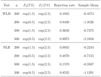
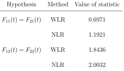
Monte Carlo data sets. If the absolute value of the normalized test statistic is greater that 1.96, we reject the null hypothesis. In table 4.3, we present the rejection rates and the sample means of normalized test statistic under different Scenarios and for
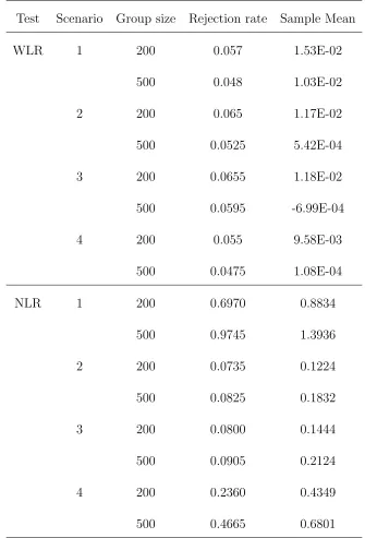
different group sizes (n= 200,500). The rejection rates are close to the nominal value 0.05 and the sample means are close to 0. Both illustrate good approximations to the large sample theory. Under each scenario the rejection rates are slightly larger than
0.05 when the sample size is 200. But when we increase the sample size to 500, they are closer to the nominal value.
We also use the Naive Log Rank (NLR) test on the same data sets we described
above, which ignores all the patients who are not consistent with treatment policies AjB1 and uses the log rank test on the available data. In table 4.3 we present the
results. From table 4.3 we can find that under scenarios 1 and 4 the rejections rates
are very large. Especially when we increase the sample size to 500 under scenario 1, the type I error increases to 0.9745! Under both scenarios 1 and 4, the distributions of the response indicator given the overall survival time for two induction groups,
Pj(R = 1|T = t), j = 1,2, are totally different. It implies that the distributions
Table 4.3: The rejection rates, sample means of test statistic under the null hypothesis and model structure B
Test Scenario Group size Rejection rate Sample Mean
WLR 1 200 0.057 1.53E-02
500 0.048 1.03E-02
2 200 0.065 1.17E-02
500 0.0525 5.42E-04
3 200 0.0655 1.18E-02
500 0.0595 -6.99E-04
4 200 0.055 9.58E-03
500 0.0475 1.08E-04
NLR 1 200 0.6970 0.8834
500 0.9745 1.3936
2 200 0.0735 0.1224
500 0.0825 0.1832
3 200 0.0800 0.1444
500 0.0905 0.2124
4 200 0.2360 0.4349
500 0.4665 0.6801
groups, Pj(Ti < t|R), j = 1,2, also are different. When we use the naive method,