Statistical Inference via Structurally and Functionally Informed Models of Protein Evolution.

(1)

ABSTRACT

WANG, KUANGYU. Statistical Inference via Structurally and Functionally Informed Models of Protein Evolution. (Under the direction of Jeffrey L. Thorne.)

Models of protein evolution tend to pay little attention to functional constraints, although structural constraints are often incorporated. Structure-informed models of protein-coding sequence evolution tend to ignore functional constraints and the pos-sibility that a protein could have more than one native conformations. This disserta-tion details the derivadisserta-tion of a structurally and funcdisserta-tionally informed model that allows protein-coding DNA evolution to be influenced by multiple tertiary structures.

The joint effects of gene expression (a functional constraint) and relative solvent accessibility (RSA), a structural constraint, in modeling protein sequence evolution are investigated in Chapter 2. Hypothesis tests are introduced to explore the relationship between RSA and codon usage at the genomic scale as well as at the individual gene scale. The genome-level results show that synonymous codons exhibit significant RSA preference bias in human. In mouse, the result is not statistically significant, possibly because of insufficient data and possibly because the relationship between RSA and synonymous codon usage is highly species-specific.

The effects of gene expression on synonymous codon usage are studied using proba-bilistic modeling. The combined effects of RSA and gene expression in influencing amino acid usage are modeled using the same probabilistic approach. Although RSA has greater influence on amino acid usage, the effect of gene expression is nevertheless significant at the synonymous codon level and should not be ignored.

(2)

(3)

(4)

Statistical Inference via Structurally and Functionally Informed Models of Protein Evolution

by Kuangyu Wang

A dissertation submitted to the Graduate Faculty of North Carolina State University

in partial fulfillment of the requirements for the Degree of

Doctor of Philosophy

Bioinformatics

Raleigh, North Carolina 2015

APPROVED BY:

David McK. Bird Steffen Heber

Celeste Sagui Jeffrey L. Thorne

(5)

DEDICATION

To my parents,

Weigang WANG and Lingping JU,

who have blessed me with their unconditional love and support. And to my wife,

Jing LI,

(6)

BIOGRAPHY

(7)

ACKNOWLEDGEMENTS

First of all, I would like to thank my advisor, Dr. Jeffrey L. Thorne, for his guidance and his patience with me in the past several years. Jeff sets an example for me both personally and academically by being an extremely nice person, a dedicated scientist and a caring friend. There is an old saying in China that “even if someone is your teacher for only a day, you should regard him like your father for the rest of your life.” With hundreds of days passed, I am so fortunate to have Jeff as an advisor. I also thank Dr. Bird, Dr. Heber and Dr. Sagui for contributing their time to serve in my advisory committee.

I would like to thank all members in Thorne group. I thank Xiang Ji for his support and collaboration in my projects. I thank Hui-jie Lee for her help with thesis proofreading. I thank Alexander Griffing for generously sharing his code and providing advice for implementation. I thank Chris Nasrallah for helping me improve presentation skills.

I also thank my friends in BRC, Yuelong Guo, Wenjing Lu, Jing Zhao, Yiwen Luo, Guozhu Zhang, Qiwen Hu and Shang Xue for their companionship.

(8)

LIST OF TABLES

Table 1.1 The instantaneous rate of change Qij for MG/GY-type models . . . . 10

Table 2.1 Test at genomic scale of whether RSA tendencies vary among synony-mous codons . . . 49 Table 2.2 Test at individual gene scale of whether RSA tendencies vary among

synonymous codons . . . 50 Table 2.3 Codons: MLR estimated coefficients for gene expression using human

data . . . 51 Table 2.4 Codons: LR estimated coefficients for expression using human data . . 52 Table 2.5 Amino acids: MLR estimated coefficients for RSA and gene expression

using human data . . . 53 Table 3.1 Test data set of ligand-binding proteins . . . 81 Table 3.2 Bayes Factor approximations for proteins in test data set . . . 82 Table 3.3 Standard deviations of posterior mean pfor sites that have highly

(11)

LIST OF FIGURES

Figure 2.1 Distance matrix for amino acids using combined human data . . . 54 Figure 2.2 Distance matrix for amino acids using stratified human data . . . 55 Figure 2.3 Predicted probabilities of amino acids across possible ranges of RSA

and gene expression . . . 56 Figure 2.4 Comparison of S = 2N s estimates between nonsynonymous and

syn-onymous point mutations to human genes . . . 61 Figure 3.1 Posterior distributions of parameter p in “shared-p” model . . . 83 Figure 3.2 Posterior means of pand widths of credibility intervals forpaccording

to the independent-p model. . . 84 Figure 3.3 Site-specific pattern of posterior mean pin “independent-p” model . 85 Figure 3.4 Alternative conformation RSA difference and posterior mean p . . . . 89 Figure 3.5 Spatial relationship of sites that have relatively strong conformation

(12)

Chapter 1 Review

One general law, leading to the advancement of all organic beings, namely, multiply, vary, let the strongest live and the weakest die.

Charles Darwin

1.1 Introduction

At the molecular scale, natural selection influences the evolution of species’ genomes at multiple levels. While nucleic acids carry the genetic information of the cell, proteins primarily execute the tasks directed by that information (Cooper, 2000). Within living organisms, proteins perform a vast array of functions . As a result, selection affects both the structure of proteins and the regulation of their production.

(13)

among proteins. Within proteins, amino acids differ in their tendencies to be associated with specific secondary structure types (Lim, 1974; Chou and Fasman, 1978). Also dif-ferent parts of a protein may contain difdif-ferent types of amino acids for other reasons, for example, the more hydrophilic amino acids would organize into protein domains that interact well with water (Stillwell, 2013).

For amino acids that are encoded by more than one codon, variations exist at the synonymous codon level. It has long been known that synonymous codons are used in different frequencies in different species (Nakamura et al., 1998). Codon usage varies among genes in a genome as well. (Sharp and Li, 1987). According to recent studies, codon-usage bias has effects on diverse biological processes, including RNA processing, protein translation and protein folding. In other words, codon usage bias has a crucial role in shaping gene expression and cellular function (Plotkin and Kudla, 2011).

Molecular phenotypes, such as protein structure and protein stability, are important links between genomic information and organismic functions, fitness, and evolution. To better understand the processes that generate protein sequences, structures, and func-tions, biologically realistic models that bring structural and functional considerations into evolutionary analyses are invaluable (Liberles et al., 2012). In this chapter, I will briefly review the development of models of sequence evolution and especially emphasize the problems that motivate my research.

1.2 Models of sequence evolution

(14)

scientists who study sequence evolution build models to investigate a few biologically realistic factors at a time and simplify other factors by making assumptions. Depending on which level of sequence information we want to focus on, a protein coding sequence can be seen as a string of 4 nucleotides, or an array of 20 amino acids, or a combination of 64 possible codons (61 codons if stop codons are excluded and the universal genetic code is used).

A predominant assumption made by most sequence substitution models is that each site in a sequence evolves independently, and substitution events at one site do not affect substitution events at other sites. With this assumption, the problem of sequence evolution breaks down into evolution of individual sites. If we can model the substitutions at one site, we can model the substitutions of entire sequence. Conventionally, a Markov chain is employed to describe the substitution process at a site. Markov models allow no “memory” in the system: the probability of change from character state i to character state j depends upon the amount of time t that has passed and the substitution rate Qij but not on character states that were visited before state i. Knowing all possible

character states, the instantaneous rate matrix Q = {Qij} that specifies instantaneous

substitution rates from one possible character state to another can be defined. Because the number of character states k at one site is finite,

Qii =− k

X

j=1,j6=i

Qij. (1.1)

According to the theory of continuous time Markov process (Karlin and Taylor, 1975), the transition probability matrix P(t) is a k×k matrix with entries denoted by Pij(t).

The Pij(t) terms are referred to as transition probabilities and represent the probability

(15)

not have the rate matrix Q change over time. With a time homogeneous process, P(t) can be calculated by matrix exponentiation:

P(t) =eQt. (1.2)

Many useful substitution models are time-reversible. A Markov model is time re-versible if and only if it satisfies:

πi×pij(t) =πj ×pji(t) for all i, j and t, (1.3)

whereπiis the stationary (equilibrium) probability of statei. If a model has this property,

there is no need to distinguish the ancestor sequence and the descendant sequence for the sake of calculating a likelihood (Felsenstein, 1981). This means that a phylogenetic tree can be rooted using any of the species or anywhere else on the tree without affecting the likelihood.

Because the chronological time duration of phylogenetic branches are typically un-known, the usual situation is that the amount of sequence change (i.e., the rate multiplied by time duration) on a branch can be inferred but this product of rates of molecular evo-lution and times cannot be disentangled into the two factors that form it. However, the conventional approach rescales evolutionary time so that it measures the expected num-ber of sequence changes per site rather than chronological time. With this rescaling and the assumption of stationarity, the average rate of change is one substitution per site. In other words, rates are typically scaled so that,

X

i

X

j6=i

(16)

Then, we can measure the amount of evolution separating two sequences by the expected number of changes between them.

1.2.1 Models of DNA substitution

Molecular sequences were scarce 40 years ago. As a result, early models for DNA were simple. Jukes and Cantor (1969) proposed the first model of DNA substitution (JC69). The basic assumption of this model is that all nucleotides have the same stationary probability πi = 1₄ and, when a nucleotide changes, it is equally likely to change to any

of the other three possible nucleotides. The resulting substitution matrix is:

Q=



       

T C A G

T −3λ λ λ λ

C λ −3λ λ λ

A λ λ −3λ λ

G λ λ λ −3λ



       

. (1.5)

If we scale the above rate matrix by the convention specified in Equation 1.4, we see that we would need λ = 4/3. However, we will illustrate this and other simple models without applying the scaling of Equation 1.4.

(17)

correspondingly. The K2P substitution matrix is: Q=         

T C A G

T −(α+ 2β) α β β

C α −(α+ 2β) β β

A β β −(α+ 2β) α

G β β α −(α+ 2β)

         . (1.6)

To relax the assumption in JC69 that nucleotide frequencies are equal, Felsenstein introduced free parameters to his model F81 to allow different nucleotide frequencies (Felsenstein, 1981). The F81 substitution rate from nucleotide itoj is set to be propor-tional toπj. Combining ideas of K2P and F81, Hasegawa, Kishino, and Yano

parameter-ized their model (HKY) as follows (Hasegawa et al., 1985):

Q=         

T C A G

T −(απC +βπR) απC βπA βπG

C απT −(απT +βπR) βπA βπG

A βπT βπC −(απG+βπY) απG

G βπT βπC απA −(απA+βπY)

         , (1.7)

where πY is the combined frequencies of pyrimidines (T and C), and πR = 1 −πY is

total frequencies of purines (A and G). A model that also permits different treatment of transitions and transversions as well as varying nucleotide frequencies but has a slightly different parameterization is the F84 model (Kishino and Hasegawa, 1989; Felsenstein and Churchill, 1996).

(18)

the most flexible one that assigns a different rate to each pair of nucleotide substitutions. Apart from πA, πC,πG and πT, there are six more parameters (α, β, γ, δ, and ε):

Q=



       

T C A G

T − απC βπA γπG

C απT − δπA πG

A βπT δπC − επG

G γπT πC επA −



       

, (1.8)

JC69, K2P, F81, HKY (and F84) can be viewed as special cases of GTR.

Felsenstein (1981) introduced a dynamic programming algorithm (often called “prun-ing algorithm”) for rapidly comput“prun-ing the likelihood of the tree, namely the probability of the observed data given tree topology, branch lengths, and parameters in the model. By making the assumption that different sites in a sequence evolve independently, the likelihood of the observed sequences arising on a given tree can be computed as the product of likelihood of sites.

(19)

according to the probability of the category.

1.2.2 Models of amino acid replacement

For many analyses, particularly for longer evolutionary distances, evolution is modeled at the amino acid level. Information is lost when we look at amino acids instead of nucleotide bases because an amino acid can be encoded by more than one codon. However, it can be advantageous to use the amino acid information in some cases. For example, DNA suffers much more from back substitutions, making it difficult to accurately estimate longer evolutionary distances. Because of that, it is more appropriate to use amino acid models when the species being studied are distantly related than it is to use nucleotide substitution models. DNA is also much more inclined to show compositional variation among evolutionary lineages than are proteins. Widely used models of DNA evolution are not easily modified to incorporate the change in nucleotide composition along an evolutionary lineage.

(20)

was employed to reconstruct the phylogenetic tree in each group. The estimated number of amino acid replacements were then used to infer relative rates of amino acid change. Because the counts came from global alignments of several protein sequences, the Dayhoff model estimates of replacement rates can be viewed as describing evolution at an average site within an average protein.

Using a similar approach but a substantially higher amount of sequence information, Jones et al. (1992) created the JTT amino acid substitution matrix. Instead of infer-ring ancestral sequences, Jones, Taylor and Thornton conducted pairwise comparisons between observed protein sequences to estimate the number of amino acid replacements. More data also allowed a more robust estimate of the probability of change between rare amino acid pairs.

1.2.3 Models of codon substitution

(21)

The first codon models were proposed by Muse and Gaut (1994) and Goldman and Yang (1994). Most codon models that are frequently used are modifications of those two models. Yang and Nielsen (2000) simplified the model of Goldman and Yang (1994) by introducing the parameterω to describe the rate ratio of nonsynonymous to synonymous changes. If we assume that synonymous substitutions are not subject to selection pressure because they do not affect the protein structure by changing the encoded amino acid, values of ω can be interpreted as the selective pressure on the protein-coding sequence. If ω is greater than 1, it means that a nonsynonymous substitution has higher rate than it would if it were a synonymous one. As a result, this substitution is selectively beneficial. If ω is less than 1, the nonsynonymous substitution is selectively deleterious. The introduction of the ω parameter makes it easier to quantify the effect of natural selection on the sequence.

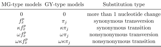
Here, models similar to Muse and Gaut (1994) are called MG-type models and models based on Goldman and Yang (1994) are referred to as GY-type models. The instantaneous rate of changeQij from codonito codonj for MG-type and GY-type of models is shown

in Table 1.1.

Table 1.1: The instantaneous rate of changeQij for MG/GY-type models

MG-type models GY-type models Substitution type 0 0 more than 1 nucleotide change

fxp πj synonymous transversion

κfxp κπj synonymous transition

ωfxp ωπj nonsynonymous transversion

ωκfxp ωκπj nonsynonymous transition

NOTE.—πj is the equilibrium frequency of a target codonj. In

contrast, fxp is the frequency of a target nucleotide.κ represents

(22)

Through analyses of mammalian and yeast sequence data, Seo and Kishino (2008) demonstrated that synonymous substitutions are very informative even for analysis of the sequences that are highly divergent. They found that codon models fit data significantly better than amino acid models, even though amino acid models account for physicochem-ical properties and codon models do not. The authors strongly recommend that protein sequence evolution to be modeled at the codon level rather than at the amino acid level. Doron-Faigenboim and Pupko (2007) developed a method to expand a 20×20 amino acid substitution matrix into a 61×61 codon matrix. This approach takes advantage of the context-dependent empirical amino acid matrices such as secondary structure–specific matrices, while the transition–transversion bias and the nonsynonymous to synonymous substitution ratio can still be taken into account. Kosiol et al. (2007) created an empirical codon model (ECM). They abandoned the assumption that no more than one nucleotide can be changed at the same time and allowed instantaneous doublet and triplet changes. To explicitly account for codon usage bias, Nielsen et al. (2007) extended Muse and Gaut (1994) and Goldman and Yang (1994) by adding the scaled selection coefficient for optimal codon usage (S = 2N s), where s is the selection coefficient acting on a substitution from an unpreferred to a preferred codon and N is the effective population size. Codons were divided into 2 categories: unpreferred and preferred. Employing results of diffusion theory from population genetics (Kimura, 1962), Yang and Nielsen calculated the fixation probability of a mutation from a preferred to an unpreferred codon as:

Ps+ =

S

(23)

and the probability from an unpreferred to a preferred codon as:

Ps− =

−S

1−es. (1.10)

Let Qij to be the MG-type/GY-type instantaneous rate of substitution, the new rate

matrix is:

Q∗_ij =



      

      

QijPs+ if i is unpreferred and j is preferred

QijPs− if i is preferred andj is unpreferred

Qij else

. (1.11)

1.2.4 Models that consider protein structure

Realizing that protein local structure environment could affect amino acid replacement rate, Koshi and Goldstein (1995) constructed substitution matrices as a function of the local structure of the protein. They incorporated parameters such as secondary structure and surface accessibility. Goldman, Thorne, and coworkers introduced an evolutionary model that combines protein secondary structure and amino acid replacement via a hid-den Markov model (Thorne et al., 1996; Goldman et al., 1996; Li et al., 1998).

(24)

Through simulations, Parisi and Echave demonstrated that simulating protein evolution via their model resulted in simulated proteins that qualitatively matched actual protein sequences in that the simulated sequences tended to have the same amino acid types at certain positions as observed in the actual proteins. This realistic variation of preferred residues among protein positions would not be generated by simulating according to other widely used models of protein change.

Building upon the technique pioneered by Parisi and Echave (2001), Robinson et al. (2003) proposed a Markov model to relax the assumption of independent change among codons. Although it is widely accepted that positions in a protein sequence do not evolve independently, dependence among sites was not incorporated into procedures for evo-lutionary inferences prior to this research. In the instantaneous rate matrix R of the Robinson model, the entry in row i and column j represents the rate of change from sequence i to another sequence j. Because the site-independence assumption was aban-doned, for a DNA sequence of lengthN nucleotides, the dimensions of rate matrix R are 4N×4N. Robinson etal.made the assumption that each substitution event changes only a single nucleotide in a residue, which helps to reduce the number of nonzero elements in each row of R to 3N + 1. Their non-zero rate matrix entries are:

Ri,j =



          

          

uπh synonymous transversion

uπhκ synonymous transition

uπhωe(Es(i)−Es(j))s+(Ep(i)−Ep(j))p nonsynonymous transversion

uπhκωe(Es(i)−Es(j))s+(Ep(i)−Ep(j))p nonsynonymous transition.

. (1.12)

(25)

model-based evolutionary approaches. The term e(Es(i)−Es(j))s+(Ep(i)−Ep(j))p _{and the} pa-rameters associated with it represent the effects on rates due to natural selection. For sequence i, Es(i) and Ep(i) denote the solvent accessibility and pairwise measures of

sequence-structure compatibility respectively. Because they are intended to be positively correlated to the free energy of the folded protein,Es(i) and Ep(i) are expected to have

low values when sequences and structures are relatively compatible. With the sequence-structure compatibility measure in place, nonsynonymous substitution rates now depend on whether the implied amino acid replacements would stabilize or destabilize the known and assumed fixed protein tertiary structure.

The high dimension (4N _×₄N_{) of rate matrix} _R _{necessitated an alternative to the}

matrix exponentiation based approach to calculate transition probabilities. To overcome this high dimensionality, the authors employed a new approach by augmenting the ob-served sequence data at tips of a phylogenetic tree with a sequence path. For every branch on the tree, the sequence path contains information about how the sequence at the be-ginning of the branch is transformed by substitution events to the sequence at the end of the branch. It also specifies the exact times of these events. Assume a tree topology that relates k observed sequences i1, i2, . . . , ik at nodes 1, 2, . . . , k. There will be I

internal nodes on this tree that are numbered k + 1, k + 2,. . . , k+I. The unobserved sequences at these nodes will be denotedik+1, ik+2,. . . , ik+I. Because Robinson model is

time reversible, for convenience, node 1 is selected as the root node and then a relative time ordering can be imposed on all nodes of the tree and the nodes that begin and end a branch can therefore be designated. Except for node 1, each node ends exactly one branch. A sequence pathρ on a tree is a collection of sequence pathsρ2, ρ3, . . . ,ρk+I on

(26)

Letting B(a) refer to the parental node of node a and letting θ represent all pa-rameters in the model including the tree topology and branch lengths, inference with a sequence path approach relies on being able to calculatep(ρa_|_iB(a)_{, θ}_{). Suppose there are}_q

substitutions along the branch pathρa_{and let}_ta₍_z_{) be the time of the}_zth _{substitution on}

this branch. Letting rate scaling parameters vary among branches, we can set times of all branches to 1 so thatta(0) = 0 andta(q+ 1) = 1. The sequence after thezth substitution on brancha is defined as ia(z). By design, ia(0) =iB(a) and ia(q+ 1) =ia(q) =ia.

R_i

_·

, the rate at which sequenceichanges to some different sequence, can be obtained by summing over Ri,j for all sequences j that differ from iby one single nucleotide. The

time interval between two consecutive substitution events is exponentially distributed with the rate parameter R_i

_·

. Given that there is a substitution affecting sequence i at some time point, the probability that i changes to j is Ri,j

R

i

·

. The sequence path density for branch a is then:

p(ia, ρa|iB(a), θ) =

q

Y

z=1

Ria₍_z₋₁₎_,ia₍_z₎ Ria₍_z₋₁₎_,_•

Ria₍_z₋₁₎_,_•e−Ria(z−1),•(t(z)−t(z−1))

!

×e−Ria(q),•(t(q+1)−t(q)) (1.13) The factor e−Ria(q),•(t(q+1)−t(q)) _{represents there not being a substitution event during} the last time period. The sequence path density over a phylogeny can be calculated by obtaining the product of all branch path densities using equation 1.13. Markov chain Monte Carlo (MCMC) techniques can be employed to jointly sample sequence paths and all other parameters θ according to their posterior probability.

(27)

Rodrigue et al. (2005) proposed to capture the complexity of protein evolution by using statistical potentials while also making use of the information available in an em-pirical amino acid replacement matrix. They also generalized the sampling technique of Robinson et al. (2003) from two taxa ton taxa.

Rodrigue et al. (2006) suggested to use Bayesian methods of model selection—based on numerical calculations of marginal likelihoods and posterior predictive checks—to evaluate site-interdependent models. Through their assessments, they found that sta-tistical potentials alone do not suitably account for differences in amino acid exchange propensities or heterogeneous rates of substitution across the sites of an alignment. For these features, the modeling strategies developed under the assumption of independence are more appropriate. They emphasized the importance to combine the use of statistical potentials with a suitably rich site-independent model.

In Rodrigue et al. (2008), the sampling of the detailed event history along each branch was improved by combining the accept-reject method described in Nielsen (2002) and the uniformization method. This hybrid approach provided a reasonably good compromise between speed and stability. The sampling method of Robinson et al. (2003) would in-volve an extensive tuning phrase in order to approximate the ratio of two intractable normalizing factors:

D(θ) D(θ0₎ =

P

ke

−2sEs(k)−2pEp(k)QN

n=1πkn

P

ke−2s

0_E

s(k)−2p0Ep(k)QN

n=1π

0

kn

(1.14)

(28)

Although site-interdependent models of protein evolution that incorporate protein structure have been shown to fit data better than the corresponding models that ignore protein structure (Rodrigue et al., 2006), state-of-the-art site-independent codon models can still achieve an even better fit to the data (Rodrigue et al., 2009). In addition, current sampling methods of the site-interdependent models are computationally intensive and thus not yet suitable for general purpose Bayesian phylogenetic applications.

Lakner et al. (2011) tested several empirical amino acid models using simple sequence-structure compatibility measures to study phylogenetic likelihood calculations under these site-independent models. Pseudo-energies for ancestral sequences from pairwise contact potentials, solvent accessibility and threading were calculated. They assessed the extent to which substitution histories that are incompatible with a protein’s three-dimensional structure contribute to the likelihood. They concluded that simple empirical substitution models may be adequate for interpolating changes between observed se-quences during phylogenetic inference.

(29)

be written as:

Qij =



              

              

0 if more than 1 nucleotide change πj synonymous transversion

πjκ(r) synonymous transition

πjω(r) nonsynonymous transversion

πjκ(r)ω(r) nonsynonymous transition

. (1.15)

The authors tested their approach using 600 yeast genes and concluded that their RSA-dependent parameters result in a better model fit than RSA-inRSA-dependent parameters.

1.2.5 Models that are connected to population genetics

Phenotype is the result of the evolutionary process, while evolution occurs in popula-tions. If parameters of interspecific models that incorporate phenotypes can be assigned population genetic interpretations, it would be possible to connect phenotype to interspe-cific evolution. The pioneering work that links population genetics to models of sequence evolution was done by Halpern and Bruno (1998). The authors defined a 64×64 substi-tution matrix at the codon level. Let r_abi be the rate that codon a is changed to codon b at position i, pab be the probability that a mutation from a to b happens at a site

(site-invariant), fi

ab be the probability that a mutation reaches fixation at site i, and k

be a scaling constant:

ri_ab=k×pab×fabi , b 6=a (1.16)

(30)

A more general interpretation of the Halpern and Bruno approach is that the rate of one sequence changing into another can be viewed as a product of two terms: the rate at which a mutation occurs and the probability that the mutation is fixed in a population. In some phylogenetic models, there are two types of parameters, the first type can be interpreted as influencing only the mutation rate and the second type can be interpreted as affecting only natural selection. These two types of parameters correspond to the mutation rate and the fixation probability respectively. In population genetics, fixation probabilities can be expressed in terms of effective population size and relative allele fitness. The Halpern and Bruno technique and its descendants (e.g., Nielsen (2003); Berg et al. (2004); Knudsen and Miyamoto (2005); Sella and Hirsh (2005); Mustonen and Lssig (2005); Thorne et al. (2007); Choi et al. (2008); Yang and Nielsen (2008)) make it possible to estimate the product of effective population size and difference in relative allele fitness from interspecific models of sequence change.

Assume we have 2N copies of allele i, any one of these alleles might give rise to a new allele j. Zij refers to the event that j is fixed in the population. Therefore, P r(Zij)

is the probability that a new mutant allele j eventually gets fixed in a population that otherwise consists of 2N −1 alleles of type i. Using the same notation as Thorne et al. (2007), the rate of sequence ito sequence j can be written as:

Rij =



      

      

uπhκ×2N ×P r(Zij) transition

uπh×2N ×P r(Zij) transversion

0 i and j differ at more than one site

. (1.18)

A few approximations of P r(Zij) are available. It is assumed that mutations are so

(31)

affected by polymorphisms at other sites. Defining sj as the difference of the relative

fitnesses of the sequences i and j, Kimura (1962) uses diffusion theory to approximate P r(Zij) as:

P r(Zij)

.

= 1−e

−2sj

1−e−4N sj. (1.19)

Sella and Hirsh (2005) came up with a more accurate than Equation 1.19:

P r(Zij)

.

= 1−e

−2log(1+sj)

1−e−4N log(1+sj). (1.20) If the above approximation is used by the model in Equation 1.18, the model will be time reversible with stationary probability:

P(j|θ) = e

2(2N−1)log(1+sj)QL

m=1πjm

P

ke2(2N−1)log(1+sk)

QL

n=1πkn

= e

2(2N−1)log(1+sj)_P

0(m|π)

P

ke2(2N−1)log(1+sk)P0(k|π)

. (1.21)

P0(m|π) is the probability of sequencemif evolution is assumed to be neutral. Choi et al.

(2008) showed that P(j|θ) in equation 1.21 can be forced to match a target probability distribution P(J) by choosing suitable selection coefficients according to:

log

P(J)/P0(J|π)

P(I)/P0(I|π)

= 2(2N −1)log(1 +sj). (1.22)

Let

τIJ =

P(J)/P0(J|π)

P(I)/P0(I|π)

, (1.23)

similar to the approximations in Halpern and Bruno (1998) and Yang and Nielsen (2008), Choi et al. (2008) reproduced that 2N × P r(Zij)

.

= logτIJ/(1− 1/τIJ) and 2N sj

(32)

(1/2)logτIJ.

The approaches described in this section successfully bridge population genetics and substitution models of sequence evolution. Based on these approaches, new models with better statistical fit can be developed. More importantly, these new models would yield a biologically plausible population genetic interpretation that can be used to understand biological systems, populations, and evolutionary processes (Thorne et al., 2007; Tamuri et al., 2012). However, some limitations remain due to the assumptions made during the modeling process. For example, it is assumed that the population size is constant, while the actual and effective population sizes can change over time. Also, the assumption that each mutation fixed or lost before next occurs is unrealistic.

1.3 Model comparison techniques

1.3.1 Akaike information criterion

The Akaike information criterion (AIC) (Akaike, 1974) is a model selection technique that is often used in a maximum-likelihood context. Let k be the number of parameters in the model and lmax be the maximized value of the likelihood in log scale, the AIC

value is defined as:

AIC = 2k−2lmax. (1.24)

(33)

Raftery et al. (2007) introduced a posterior simulation-based analog of the AIC cri-terion referred to as AICM. One advantage of AICM is that it can be estimated directly from posterior samples generated by Markov chain Monte Carlo (MCMC), a class of algorithms for sampling from a probability distribution based on constructing a Markov chain that has the desired distribution as its equilibrium distribution. Letting ¯l and s2

l

be the sample mean and variance of the posterior log likelihoods, Raftery et al. showed that k can be estimated by 2s2_l and lmax can be estimated by ¯l+s2l. As a result, AICM

can be estimated as:

AICM = 2k−2lmax

= 2(2s2_l)−2(¯l+s2_l)

= 2¯l−2s2_l. (1.25)

1.3.2 Bayes factor

The evaluation of Bayes factors (BFs) is considered as a standard approach to perform model comparison in a Bayesian phylogenetic framework (Suchard et al., 2001). The marginal likelihood is the probability of observing the data given a specific model. LetD to represent observed data while M0 and M1 are two different models under comparison.

Then, the BF is a ratio of two marginal likelihoods:

BF = P r(D|M1) P r(D|M0)

. (1.26)

(34)

Harmonic mean estimator

The harmonic mean estimator (HME) (Newton and Raftery, 1994) is the simplest method to estimate the marginal likelihood of the posterior distribution. Ifxrepresents the entire dataset,θ is the entire set of parameters andθ1,θ2, . . . ,θnare samples from the posterior

distribution, HME can be computed as:

HME = ₁ n

P(x|θ1) +

1

P(x|θ2) +· · ·+

1

P(x|θn)

= _P_n n

i=1 1

P(x|θi)

. (1.27)

The HME has been used extensively in the field of phylogenetics. For the HME to gen-erate good estimates, an unrealistically large number of samples need to be obtained. As a result, HME is often severely biased, overestimating the true marginal likelihood, especially when the model has higher dimension (Xie et al., 2011). For this reason, the HME should be avoided when Bayes Factor approximations are desired (Lartillot and Philippe, 2006).

Path sampling

Originating from theoretical physics, path sampling (Ogata, 1989; Gelman and Meng, 1998) is a method for high-dimensional integration that addresses the problem of marginal likelihood calculation. Letθbe parameter space withZ0 =P r(D|M0) andZ1 =P r(D|M1),

the goal here is to obtain a numerical evaluation of:

log(BF) = log

Z1

Z0

(35)

According to Bayes’ theorem, the true probability densities are:

P(θ|D, Mi) =

P(D|θ, Mi)P(θ|Mi)

P(D|Mi)

. (1.29)

Let q0(θ) = P(D|θ, M0)P(θ|M0) and q1(θ) = P(D|θ, M1)P(θ|M1):

Zi =

Z

θ

qi(θ)dθ, i= 0,1 (1.30)

are the normalization constants. The key idea is to define a continuous and differentiable path:

qβ(θ) = [P(D|θ, M0)P(θ|M0)]1−β[P(D|θ, M1)P(θ|M1)]β, (1.31)

that connects q0 and q1. When β = 0, qβ(θ) is equal to q0(θ), and when β = 1, qβ(θ) is

equal to q1(θ). Zβ is defined as:

Zβ =

Z

θ

qβ(θ)dθ. (1.32)

It has been shown by Lartillot and Philippe (2006) that

log(BF) = log

Z1

Z0

(1.33)

=

Z 1

0

∂logZβ

∂β dβ (1.34)

=

Z 1

0

Eβ

∂logqβ(θ)

∂β

dβ (1.35)

=

Z 1

0

Eβ[U]dβ. (1.36)

(36)

between 0 and 1. Using MCMC, a collection of samples (βk, θk)k=0...K can be obtained.

Eβ[U] can be evaluated by calculating averages of these samples.

Xie et al. (2011) introduced a method called stepping-stone sampling that combines ideas from both importance sampling and path sampling. The marginal likelihood is esti-mated in a series that bridges the posterior and prior distributions of a model. Baele et al. (2012) showed that path sampling and stepping-stone sampling consistently outperform the AICM and HME for evaluating evolutionary models.

1.4 Structural and functional constraints that affect

protein evolution

Protein evolution is subject to natural selection, while natural selection depends on the stringency of functional or structural constraints. There is a rich body of literature docu-menting constraints from different sources. For the purpose of this thesis, gene expression, a functional constraint, and protein alternative conformations, a structural constraint, will be discussed in this section.

1.4.1 Gene expression

(37)

A classic point of view is that highly expressed proteins are selected to achieve faster translation rates and high accuracy by using “optimal codons” where “optimal codons” are the codons with most abundant tRNAs in a set of synonymous codons. The “optimal codons” are thought to be more robust against translation errors. With this perspective, fitness advantage is achieved through increased translation efficiency (Ikemura, 1982) or accuracy of protein synthesis (Akashi, 1994; Drummond and Wilke, 2008).

To explain consistent correlations between rates of coding-sequence evolution and gene expression levels across taxa, Drummond and Wilke (2008) suggested that mistranslation-induced protein misfolding is a dominant constraint on coding-sequence evolution. Zhou et al. (2009) found translationally optimal codons often encode buried residues. They also found translationally optimal codons at protein locations where non-synonymous mutations lead to large changes in free energy. These findings indicate that coupling mechanisms may exist between structural and functional constraints.

Highly expressed genes are often involved in many protein–protein interactions, lead-ing to a possible conflict between increaslead-ing the strength of functional interactions and avoiding misinteractions (Heo et al., 2011). The evolution of highly expressed protiens could be further constrained by this conflict.

1.4.2 Protein alternative conformations

(38)

conformation to another. For example, ligand-binding proteins carry out their functions by changing their tertiary structure upon binding ligands. In other cases, a single protein can also exist in more than one conformation independent of any conformational changes induced by ligand binding (e.g., James and Tawfik (2003)). The cytokine lympho-tactin (Tuinstra et al., 2008) and the cell cycle control protein Mad2 (Luo et al., 2004) are two such examples.

It has been proposed that conformational diversity may facilitate protein evolution and helps to account for the origins of new biological functions (Meier et al., 2007). In par-ticular, proteins with two alternative native-state conformations (bi-stable proteins) are hypothesized to function as evolutionary bridges at the interface between two groups of protein sequences that fold uniquely into the two different native conformations (Sikosek et al., 2012).

The Elastic network model (ENM) describes a protein as a network of nodes connected by springs (normal modes). The ENM can help to deduce conformational flexibility and dynamics of protein conformation transitions to a reasonable degree (Micheletti et al., 2002; Zheng et al., 2006; Zen et al., 2008). Protein motions such as transitions between ligand-free and ligand-bound conformations can usually be represented using one or a few low-energy normal modes (Bahar et al., 2010). By applying ENM to a set of globin-like proteins, Echave (2012) suggested that the physical explanation of the conservation of lowest normal modes is their robustness against random mutations.

(39)

bioin-formatics tools to be developed to take into account the substitution bias caused by alternative conformations.

(40)

Chapter 2 Role of solvent accessibility and

gene expression in modeling protein

sequence evolution

2.1 Abstract

(41)

model. Instead of focusing on parameter estimation, we concentrate on the population genetic implications of this model. Specifically, we obtain estimates of 2N s, the product of effective population size N and relative fitness difference of alleles s. For a training data set consisting of human proteins with known structures and expression data, 2N sis estimated separately for synonymous and nonsynonymous substitutions in each protein. We then contrast the patterns of synonymous and nonsynonymous 2N sestimates across proteins while also taking gene expression levels of the proteins into account.

2.2 Introduction

Proteins perform a vast array of functions within living organisms. As a result, natural selection affects both the structure of proteins and the regulation of their production. A major source of structural constraints arises because proteins require a stable and suitable three-dimensional structure to function. Mutations that destabilize proteins will be selected against (DePristo et al., 2005). Also, selective constraints in a protein vary according to structural locations. For example, Franzosa and Xia (2009) found a strong, positive and linear relationship between the ratio of nonsynonymous and synonymous rate and relative solvent accessibility (RSA). While structural constraints have mainly been investigated to explain nonsynonymous rate variation within proteins, functional constraints have been shown to explain a large amount of the variation in average non-synonymous rate among proteins (Pal et al., 2001; Drummond et al., 2005, 2006). For example, Drummond et al. (2005) showed that expression level explains roughly half the variation in average nonsynonymous rate amongSaccharomyces cerevisiae protein-coding genes.

(42)

sim-ulation work of Parisi and Echave (2001) had a statistical potential govern the amino acid replacement process. A similar approach was adopted by later inferential studies (Robinson et al., 2003; Rodrigue et al., 2006; Kleinman et al., 2006; Rodrigue et al., 2009). Statistical potentials can include terms related to solvent accessibility, pairwise distance interactions, torsion angles, and flexibility of the residues (e.g., see Kleinman et al., 2010).

Structurally constrained evolutionary models have tended to place less emphasis on codon usage. The assumption that synonymous mutations are selectively neutral has often been made (e.g., Robinson et al., 2003; Rodrigue et al., 2006, 2009). This may be a reasonable first assumption, because so much natural selection depends on the protein sequence. However, synonymous change is also affected by natural selection. For example, Agashe et al. (2013) found that synonymous mutations to a key-enzyme coding gene can decrease gene expression and fitness by more than 90% compared to wild-type. Also, selection acting on gene expression was found to be the single dominant predictor, among all predictors considered, of the number of nonsynonymous substitutions per site in yeast (Drummond et al., 2005).

To explain the negative correlations between rates of coding sequence evolution and gene expression levels that have been inferred across a wide range of taxa, Drummond and Wilke (2008) suggested that mistranslation-induced protein misfolding explains much of coding sequence evolution. Another study discovered that translationally optimal codons are associated with structurally sensitive sites (Zhou et al., 2009). These findings indi-cate that structural and functional constraints are coupled. While protein structures are increasingly considered in protein evolution models, less attention has been paid to the combined effect of gene expression and protein structure.

(43)

(Sharp et al., 1995). Chen et al. (2004) concluded that different patterns of codon usage between species are determined primarily by mutational processes that act throughout the genome, and only secondarily by selective forces acting on protein coding sequences. From a selectionist point of view, a classic explanation for systematic variation across a genome is that certain preferred codons are translated more accurately and/or efficiently (Jia and Higgs, 2008; Higgs and Ran, 2008; Hershberg and Petrov, 2008). Strong evidence for this hypothesis has been found in several species (Post and Nomura, 1979; Ikemura, 1981, 1982; Moriyama and Powell, 1997; Duret, 2000). However, 30% of bacterial species show no evidence of translational selection (Sharp et al., 2005). Understanding codon usage patterns continues to be an active area of research.

(44)

assessed by our estimates of scaled selection coefficients (i.e., twice the product of effec-tive population sizeN and the relative fitness difference s between the mutant and wild type allele).

2.3 Materials and Methods

2.3.1 Structural, sequence and expression Data

We collected protein structures, amino acid sequences, nucleotide sequences and protein-coding gene expression data for two species,H. sapiens and M. musculus. Protein struc-tures were obtained from the PDB database (Berman et al., 2000). Only strucstruc-tures determined by X-ray crystallography with a resolution of 3.0 ˚A or better were employed. We restrict our data to monomeric proteins with one chain. In addition, proteins were required to have lengths greater than 50. Membrane proteins and protein-DNA/RNA hybrid structures were excluded. Homologs were removed from our data by employing a 30 percent identity filter.

Because the Consensus CDS (CCDS) Database (Pruitt et al., 2009) stores a core set of human and mouse protein-coding regions that are associated with highly reliable anno-tation, it was used to identify nucleotide sequences that encode the proteins selected from PDB. To get CCDS IDs, protein PDB IDs were translated to the UniProt Knowledgebase (UniProtKB) IDs. The Uniprot IDs were then mapped to Gene IDs. Finally, Gene IDs were converted to CCDS IDs. Proteins with CCDS IDs that could not be successfully identified were removed.

(45)

program from the EMBOSS tools (Rice et al., 2000). This let us identify the longest ungapped region with an exact match between the nucleotide sequence and amino acid sequence. For each site in the ungapped region in each protein structure, relative solvent accessibility was calculated by the NACCESS software (Hubbard and Thornton, 1996). This process yielded 864 and 156 matches in H. sapiens and M. musculus, respectively.

RNA-seq data forH. sapiensandM. musculus were collected as part of a multi-species multi-organ gene expression study (Brawand et al., 2011) and were downloaded from the Expression Atlas Database (Petryszak et al., 2014). To establish one-to-one mapping between the PDB ID of a protein and the Ensembl ID of a transcript, PDB IDs were translated to the UniProtKB IDs and then the Uniprot IDs were mapped to Ensembl IDs via the ID mapping service hosted by the Protein Information Resource (Wu et al., 2003). Following a previous study by Drummond and Wilke (2008), aggregate mRNA level was quantified as the geometric mean signal of the measurements from the 6 tissues in the Brawandet al. data set. We log-transformed these geometric means in the following analysis. There are 241 human proteins and 60 mouse proteins in our data set that have both structure and gene expression information available.

(46)

context, and the functional context. For a codon C of a protein sequence, let A be the amino acid encoded by this codon. Here, R will be the relative solvent accessibility at the site and will represent the structural context while E will be the expression level of the gene and will represent the functional context. The probability of obtaining C conditional upon the context is then:

P(C|R, E) =P(C|A, R, E)·P(A|R, E). (2.1)

Testing association between codon usage and RSA

Codon usage is correlated with gene expression (e.g., Hershberg and Petrov, 2008). Fur-thermore, amino acid usage is RSA-dependent (e.g., Franzosa and Xia, 2009; Ramsey et al., 2011; Yeh et al., 2013) and also influenced by gene expression (Herbeck, 2003; Schaber et al., 2005). Zhou et al. (2009) tested the association between codon optimality and solvent accessibility. Instead of focusing on codon optimality which primarily reflects the influence of selection for translation speed and/or accuracy on codon usage, we test a slightly more general null hypothesis that, conditional upon the amino acid, codon usage is independent of RSA.

(47)

test statistics were generated via this sort of permutation. The actual computation was done with the “ad.test” function in the R package “kSamples” (Scholz and Stephens, 1987).

We can test whether RSA distributions of synonymous codons are different either at the genomic scale or at the individual gene scale. At the genomic scale, for each of the 18 amino acids that have more than one codon, a k-sample A-D test was conducted. Positions in all genes that have the same amino acid type were pooled together and RSA values were permuted among these positions. In each test, the null distribution was formed by the 10,000 simulated A-D test statistics. To get the p-value, the test statistic computed from observed data is compared to the null distribution and the proportion of the null distribution that exceeds the observed test statistic value is recorded. At the genomic scale, we have the power to detect even slight violations of the null hypothesis. A disadvantage of the genomic-level test is that permuted data sets do not retain the same codon usage patterns as the actual data. This means that association between codon usage and gene expression is disrupted in the permuted data sets.

(48)

sample standard deviation. For each amino acid type, the 10,000×864 and 10,000×156 z-scores were summed across proteins so that 10,000 sum-of-z-scores (the combined null distribution) were obtained in human and in mouse. Finally, we compute p-values by comparing the observed sum-of-z-score for an amino acid with the corresponding null distribution. Although testing at the gene scale allows gene-specific codon bias to be removed, there is less power to reject the null hypothesis at the individual gene scale because each gene has a comparatively small number of codons for each amino acid.

Clustering amino acids according to RSA preference

The RSA of an amino acid residue in a protein is affected by tertiary structure of the protein, apart from the amino acid’s physicochemical properties (Kim and Park, 2004). Before we proceed to quantitative modeling, we would like to find out how interchange-able two amino acids are in terms of RSA distribution and whether amino acids can be grouped together by their RSA distribution similarities. The two-sample KolmogorovS-mirnov (KS) test is one of the most useful and general nonparametric methods for com-paring two samples. In other contexts (Pauwels and Frederix, 2000; Volkovich et al., 2010; Zhang and Boutros, 2013), the K-S test statistic has been used to define distances for the purpose of hierarchical clustering. Borrowing the idea from hypothesis testing, we define the distance between a pair of amino acids by the normalized two-sample KS test statistic (Equation 2.2) when contrasting their RSA distributions. We let n and n0 be samples sizes for each amino acid type and we obtain a test statistic:

normalized KS statistic = supx|F1,n_q(x)−F2,n0(x)|

n+n0

nn0

(49)

where F1,n and F2,n0 are the empirical RSA distribution functions of the two amino acids respectively. Similar to hypothesis testing for codon usage, an amino acid distance matrix can be constructed either at the genomic scale or the individual gene scale. For the latter, one distance matrix can be computed within each protein and all matrices can be combined by taking element-wise means. Complete-linkage clustering (Sorensen, 1948) is employed to find the grouping pattern in a distance matrix.

Logistic regression

If there is no significant association between codon usage and RSA, we can make the following simplification to Equation 2.1:

P(C|A, R, E) = P(C|A, E). (2.3)

Since we are interested in understanding how gene expression (a predictor variable) affects probabilities of amino acid types (a categorical outcome variable), logistic regression (in cases where there are exactly two synonymous codons) and multinomial logistic regression (MLR) can be employed. The most frequent codon in each synonymous group is denoted Cr and the probability of any other synonymous codon C is modeled relative to it:

log

P(C|A, E) P(Cr|A, E)

=α+βC ·E (2.4)

where α is the intercept, and βC is the slope for gene expression with codon C. When

(50)

To measure the joint effect of RSA and gene expression on amino acid usage quan-titatively, we use both gene expression and RSA as independent variables and build a model similar to the one in Equation 2.4 but this time the probabilities are relative to Ar, the reference amino acid:

log

P(A|R, E) P(Ar|R, E)

=α+βR,A·R+βE,A·E (2.5)

whereβ1,A,β2,A are the slopes for amino acidA of RSA and gene expression respectively.

The most frequent amino acid (in our case, leucine) is chosen as Ar. A likelihood ratio

test can compare the full model in Equation 2.5 with reduced models in Equation 2.6 and 2.7.

log

=α+βR,A·R (2.6)

log

=α+βE,A·E (2.7)

2.3.3 A functionally and structurally constrained Markov model

of codon substitution

Using the probabilistic framework that we have constructed, we develop a model of protein-coding DNA sequence evolution that explicitly accounts for structural and func-tional constraints.

The rate of change from codonito codonj will be denotedqij. Our mutation-selection

balance parameterization has each substitution rate be proportional to the mutation rate fromi toj multiplied by the probability that a new mutation becomes fixed. We denote πk as the stationary probability of nucleotide typek (k ∈ {A, C, G, T}) in the absence of

(51)

κ be the transition–transversion rate ratio. Assume a diploid population of effective size N individuals and let P(Zij) be the probability that a new mutant allele j eventually

gets fixed in the population that otherwise consists of 2N −1 alleles of type i. We set qij to 0 if i or j is a stop codon or i and j differ by more than one nucleotide. When i

and j differ by exactly a single codon position and codonj has nucleotide type hat this position, our model specifies the substitution rate qij from codoni to codon j as

qij =



  

  

uπh×2N ×P(Zij) transversion

uπhκ×2N ×P(Zij) transition,

(2.8)

where the scale factoru is defined by the requirement that the average substitution rate for a codon substitution process at stationarity is one.

Following Choi et al. (2008), we design our evolutionary model to have a stationary distribution that matches a desired target probability distribution. In this case, we have our evolutionary model to yield a stationary distribution that is identical to the proba-bility distribution of codons that we estimated via multinomial logistic regression from solvent accessibility and gene expression data of human proteins. Accordingly, we set P(i|R, E) as the stationary probability for codon i. It can be calculated using Equations 2.1, 2.4 and 2.5.

LetP0(i|π) be the probability of codon i under a model where stop codons are lethal

but all other codons are equally fit. Adjusting for the 3 stop codons in the universal genetic code,

P0(i|π) =

πi1πi2πi3

1−πTπAπA−πTπAπG−πTπGπA

(52)

According to the approximation introduced in Choi et al. (2008),

τij =

P(j|R, E)/P0(j|π)

P(i|R, E)/P0(i|π)

(2.10)

and

2N ×P(Zij) =

log(τij)

1−1/τij

, (2.11)

yield a Markov model that is time-reversible. One advantage of our model is that the number of parameters that are introduced in the effort to include RSA and gene expres-sion is small. The trade-off is that our model will incur extra computation because RSA values can be different from site to site. We need to have one rate matrix for each site, although these rate matrices can share parameters such as κ.

The scaled selection coefficient can be assessed by (Halpern and Bruno, 1998; Yang and Nielsen, 2008; Choi et al., 2008):

S = 2N s= 1

2·log(τij). (2.12)

(53)

πA = πT = 0.59/2 = 0.295 and πC = πG = 0.41/2 = 0.205. This treatment could be

improved by allowing π to vary among genes to account for regional genomic differences in mutation patterns, but it is not pursued in this study.

2.4 Results

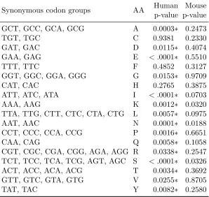
After using the Benjamini-Hochberg (BH) method (Benjamini and Hochberg, 1995) to control for false discovery rate, no synonymous codon group in mouse was found to exhibit a significant correlation between codon usage and RSA. In contrast, 15 out of 18 synonymous codon groups in human were statistically significant (Table 2.1). For humans, the null hypothesis cannot be rejected in synonymous codon groups belonging to cysteine (C), phenylalanine (F), histidine (H).

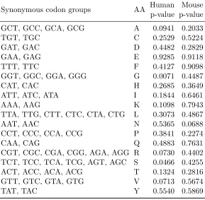
When the same hypothesis was tested at the individual gene level, the p-value results can be found in Table 2.2. After applying the BH method, no synonymous codon group was found to be statistically significant in either human or mouse, although p-values in human are consistently smaller than those in mouse.

(54)

are also present. As explained in the Materials and Methods section, we also constructed another distance matrix using data stratified by each gene. We computed one distance matrix for each protein in our data set and then calculated the average values for each cell in the distance matrix across all proteins. The resulting distance matrix is shown in Figure 2.2. The same clustering pattern was found as in Figure 2.1, although the signal is weaker due to the much smaller sample sizes in individual protein-coding genes.

Multinomial logistic regression results

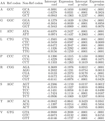
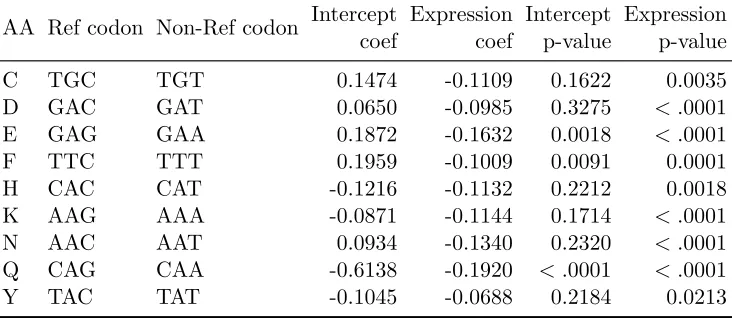
Using human data, the estimated coefficients of multinomial logistic regression (MLR) models for synonymous codon groups with more than two codons are shown in Table 2.3. For groups with exactly two synonymous codons, estimated coefficients of logistic regres-sion (LR) models are in Table 2.4. The estimates of the slope parameter for log-scaled gene expression are all negative for LR models and they are all statistically significant. Across all MLR models, 24 out of 32 slope estimates for gene expression are negative and statistically significant, while only one coefficient belonging to codon TCG in amino acid serine is positive and significant. Since we define the most frequent (also called “pre-ferred”) codon to be the reference category in both MLR and LR cases, these estimates coincide with findings from earlier studies (e.g., Ikemura, 1981; Duret, 2000; Hiraoka et al., 2009) that the probability of observing the most frequent codon increases when gene expression level is higher (with one exception).

(55)

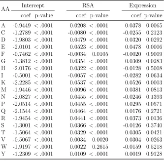
and isoleucine), slope estimates for RSA of the non-reference amino acids are positive. This means that the relative probability of observing these amino acids rather than the reference amino acid leucine is higher as RSA increases, holding gene expression identical. To depict a full picture of the joint effect of RSA and gene expression, heatmaps are shown in Figure 2.3 to present the predicted probabilities of each amino acid. While RSA plays a dominant role in determining the region of high probabilities for amino acids such as leucine, phenylalanine and proline, the effect of gene expression is evident in cases such as histidine, asparagine and serine.

“Scaled” selection coefficients

(56)

2.5 Discussion

We developed a probabilistic framework that simultaneously considers RSA (a struc-tural constraint) and gene expression (a functional constraint). By design, the two-step construction process of this framework (Equation 2.1) captures codon usage bias at the nucleotide level as well as structural-and-functional dependence of amino acids.

Hypothesis testing at a genomic scale reveals a potentially species-specific difference in the relationship between synonymous codon choice and RSA. In humans, the null hypothesis that RSA is independent of synonymous codon choice can be rejected. In mouse, the result is not statistically significant, possibly because of insufficient data and possibly because the relationship between RSA and synonymous codon usage is less strong. At the individual gene level, we test the same hypothesis using permutation and resampling. Although we fail to reject the null hypothesis in both human and mouse, we notice that the association between RSA and codon usage is stronger in human than in mouse. This is consistent with our finding at the genomic scale. Because we derive one test statistic from each gene and combine the test statistics to get an overall test statistic and its null distribution, we are treating each protein equally. However, due to small sample size, the test statistics calculated in some proteins may not be informative and can contribute stochastic noise to the combined test statistic. Improved test statistics might yield different conclusions.

(57)

in this step, because our analyses indicate that the correlation between RSA and codon usage is small to nonexistent. This does not mean that there is no structure constraint on codon usage. Protein structure may lead to selection pressure on synonymous codon choice through an interaction between the translation process and protein folding (Scher-rer et al., 2012). Codon usage is also subject to other constraints, because it can affect splicing and/or mRNA stability (Chamary et al., 2006).

To predict amino acid types, we incorporate both RSA and gene expression as in-dependent variables in our MLR model. Our likelihood ratio test confirms that the full model with both variables fits data significantly better than reduced models. Although the impact of gene expression on amino acid probabilities is weaker than the impact of RSA, it is still significant. In Figure 2.3, the heatmaps for amino acids such as glycine, histidine, and serine show that these amino acids reach their highest probabilities at intermediate RSA values.

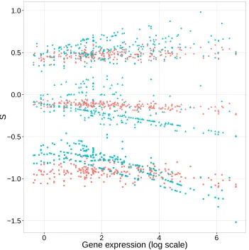
We observed a trend that 2N s estimates for both nonsynonymous and synonymous point mutation become more negative as gene expression increases (Figure 2.4). This observation is biologically reasonable and a few mechanisms might contribute to it. Highly expressed proteins have been found to evolve slower due to the stronger selection pressure that they experience (Drummond et al., 2005; Drummond and Wilke, 2008; Serohijos et al., 2012). Many highly expressed proteins are functionally important or even essential. For those proteins, the cell cannot afford their function to be disturbed or their abundance to become low (Sikosek et al., 2012).

(58)

selec-itative pattern remains when we restrict consideration to synonymous point mutations. For these mutations, 64.0% yield negative values. Among nonsynonymous mutations, 64.3% of possible point mutations are inferred to be deleterious.

However, the distribution of nonsynonymous scaled selection coefficient estimates is clearly unrealistic in that it is too tightly clustered around the value of 0. Because some possible nonsynonymous mutations are lethal or at least highly deleterious, there should be some scaled selection coefficient values that are far below 0. We do not observe this expected long lower tail of the distribution of scaled selection coefficients for nonsynony-mous point mutations (e.g., see the 5% nonsynonynonsynony-mous values in Figure 2.4). Because some nonsynonymous mutations should be extremely deleterious, we also expect the av-erage over all possible nonsynonymous mutations to be substantially below zero. We do not observe this. In fact, the average estimates of 2N s for nonsynonymous mutations is about -0.162 and this is only slightly less than the -0.158 value represent the average 2N sestimate among synonymous point mutations. Similar shortcomings have been noted for distributions of scaled selection coefficients that have been inferred via a mutation-selection balance model of molecular evolution (Thorne et al., 2007; Choi et al., 2008). Much of the mismatch between our expectations and our estimates is likely due to flaws of our evolutionary model. Specifically, the rates in our model depend on the RSA and gene expression covariates but other aspects of phenotype are clearly very relevant to natural selection and are not captured by our model.

(59)

po-tentially important to consider when connecting interspecific models of sequence change to population genetics (Cartwright et al., 2011).

(60)

2.6 Tables

Table 2.1: Test at genomic scale of whether RSA tendencies vary among synonymous codons

Synonymous codon groups AA Human Mouse p-value p-value GCT, GCC, GCA, GCG A 0.0003∗ 0.2473

TGT, TGC C 0.9381 0.2330

GAT, GAC D 0.0115∗ 0.4074

GAA, GAG E < .0001∗ 0.5510

TTT, TTC F 0.4852 0.3127

GGT, GGC, GGA, GGG G 0.0153∗ 0.9709

CAT, CAC H 0.2765 0.3875

ATT, ATC, ATA I < .0001∗ 0.0703

AAA, AAG K 0.0012∗ 0.0320

TTA, TTG, CTT, CTC, CTA, CTG L 0.0057∗ 0.0975

AAT, AAC N 0.0001∗ 0.0188

CCT, CCC, CCA, CCG P 0.0016∗ 0.6651

CAA, CAG Q 0.0058∗ 0.1058

CGT, CGC, CGA, CGG, AGA, AGG R 0.0338∗ 0.2547 TCT, TCC, TCA, TCG, AGT, AGC S < .0001∗ 0.0326 ACT, ACC, ACA, ACG T 0.0034∗ 0.3692 GTT, GTC, GTA, GTG V 0.0255∗ 0.8705

TAT, TAC Y 0.0082∗ 0.2580

Statistical Inference via Structurally and Functionally Informed Models of Protein Evolution.

ABSTRACT

DEDICATION

BIOGRAPHY

ACKNOWLEDGEMENTS

TABLE OF CONTENTS

LIST OF TABLES

LIST OF FIGURES

Chapter 1

Review

1.1

Introduction

1.2

Models of sequence evolution

1.2.1

Models of DNA substitution

1.2.2

Models of amino acid replacement

1.2.3

Models of codon substitution

1.2.4

Models that consider protein structure

·

·

·

1.2.5

Models that are connected to population genetics

1.3

Model comparison techniques

1.3.1

Akaike information criterion

1.3.2

Bayes factor

1.4

Structural and functional constraints that affect

protein evolution

1.4.1

Gene expression

1.4.2

Protein alternative conformations

Chapter 2

Role of solvent accessibility and

gene expression in modeling protein

sequence evolution

2.1

Abstract

2.2

Introduction

2.3

Materials and Methods

2.3.1

Structural, sequence and expression Data

2.3.3

A functionally and structurally constrained Markov model

of codon substitution

2.4

Results

2.5

Discussion

2.6

Tables

_·

_·