A method of screening for genes of major effect.

A

Method of Screening for Genes of

Major Effect

B. P.

Kinghorn,*

B. W.

Kennedyt

and

C.

Smith?

*Department of Animal Science, University of New England, Australia, and tCentre for Genetic Improvement of Livestock, University of Guelph, Canada

Manuscript received January 15, 1992 Accepted for publication December 28, 1992

ABSTRACT

This paper describes a method for screening animal populations on an index of calculated probabilities of genotype status at an unknown single locus. Animals selected by such a method might then be candidates in test matings and genetic marker analyses for major gene detection. The method relies on phenotypic measures for a continuous trait plus identification of sire and dam. Some missing phenotypes and missing pedigree information are permitted. The method is an iterative two-step procedure, the first step estimates genotype probabilities and the second step estimates genotypic effects by regressing phenotypes on genotype probabilities, modeled as true genotype status plus

error. Prior knowledge or choice of major locus-free heritability for the trait of interest is required, plus initial starting estimates of the effect on phenotype of carrying one and two copies of the unknown gene. Gene frequency can be estimated by this method, but it is demonstrated that the consequences of using an incorrect fixed prior for gene frequency are not particularly adverse where true frequency of the allele with major effect is low. Simulations involving deterministic sampling from the normal distribution lead to convergence for estimates of genotype effects at the true values, for a reasonable range of starting values, illustrating that estimation of major gene effects has a rational basis. In the absence of polygenic effects, stochastic simulations of 600 animals in five generations resulted in estimates of genotypic effects close to the true values. However, stochastic simulations involving generation and fitting of both major genotype and animal polygenic effects showed upward bias in estimates of major genotype effects. This can be partially overcome by not using information from relatives when calculating genotype probabilities-a result which suggests a route to a modified method which is unbiased and yet does use this information.

S

EVERAL genes of major effect and commercial value have been discovered by animal breeders. It seems that inspection of data and partly intuitive deduction have been the root of most or all of these discoveries. HOESCHELE (1 988) presented a method which uses modal values of joint and marginal poste-

rior distributions to simultaneously estimate polygenic effects and major genotype status. This method re-

quires the development of likelihood equations alge- braically tailored to the structure of the prevailing data set, which will make application difficult in many cases. HOESCHELE’S method and other approximate

maximum likelihood methods (KNOTT, HALEY a n d

THOMPSON 1 9 9 l a , b ; HOFER a n d KENNEDY 1993) have been tested on simulated half-sib data sets. T h i s paper presents a different approach which is simpler to apply for data sets running over several generations, with missing phenotypes and missing pedigree information.

OVERVIEW OF METHOD

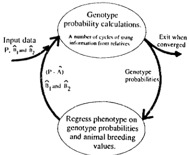
T h e m e t h o d is an iterative two-step procedure, as illustrated in Figure 1 . T h e first step estimates geno- type probabilities at an unknown locus. T h e second step estimates genotypic effects (the effect of carrying one copy, P I , and the effect of carrying two copies,

Genetics 134: 351-360 (May, 1993)

&, of the major gene) by regressing phenotypes on genotype probabilities, modelled as true genotype sta- tus plus error.

T h e power of any method which does not use genetic markers is not sufficient to have it touted as a tool to detect single genes. We propose that such

methods will have practical value in preliminary screening of populations to select animals for gene detection using more powerful approaches. Thus a simple test will be made in this paper for the method’s

ability to capture major genes in a screening process.

GENOTYPE PROBABILITY ESTIMATION

The method used here, “the continuous method.” is based largely on the iterative “discrete method” of

VAN ARENDONK, SMITH a n d KENNEDY (1 989). The

benefit of VAN ARENDONK’S method compared to

probahility calculations.

u

and animal breeding

values.

FIGURE 1.-An illustration of the method used for stochastic simulations and real data to arrive at converged estimates of major gene effects, Dl and p2, and calculate genotype probabilities for individuals. Genotype probabilities are calculated following the method of VAN ARENDONK, SMITH and KENNEDY (1989) described in the text. These are then fitted in a regression of phenotype on

genotype probabilities and animal breeding values as described in the text. This regression yields estimates of breeding value and new estimates of /31 and &. Phenotypes (P) are corrected for estimated breeding values

(a)

in an attempt to reduce the influence of polygenic effects on the next calculation of genotype probabilities. T h e cycle illustrated is repeated sufficient times to give convergence in estimates of 0, and

&.

However, to speed operation, convergence is first achieved with animal breeding values not fitted in the regressions, then animal breeding values are fitted until final con- vergence is reached.

T h e continuous method uses information on phe- notypes of continuous measures, and does not assume knowledge of the effect of different genotypes at the locus concerned. The two methods are thus appropri- ate to two different types of data.

When only the phenotype y of the individual is

known, the probability of that individual having gen- otype u is, from VAN ARENDONK, SMITH and KENNEDY

(1 989):

where prob(u) = probability of the individual having genotype u, prior(u) = prior probability of the indi- vidual having genotype u (found simply according to the prior estimate of gene frequency), and

k =

3 is the number of possible genotypes.

In the discrete method, g(yl u ) is the conditional probability of phenotype y given genotype u . This is

quite simple to derive. For example, where each gen- otype is uniquely associated with a different pheno- type, then g(y

I

u ) = l where y is the phenotype asso- ciated with u , and it equals zero in all other cases. Prior knowledge of the mode of inheritance is re- quired.

I n the continuous method, g(ylu) is the height of the normal distribution

Nbx,

a:) at phenotypey, where

I'lsnoty;e

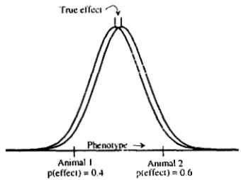
FIGURE 2.-An illustration of the relationship between pheno- type and probability of belonging to the distribution of animals expressing a positive effect. T h e effect equals two within-group standard deviations, and 25% of the population expresses the effect. This example relates to either a haploid organism with two gene types at the single locus, or to a diploid organism with three genotypes but complete dominance of one allele.

5

is the mean phenotype of genotype u individuals and u: is the phenotypic variance within genotype u.

This presentation assumes normal distribution of phe- notypes about the mean genetic values of the three major-locus genotypes involved, but prior knowledge of an alternative form of distribution can be accom- modated simply. In the method presented in this paper, these mean genetic values are estimated from the data. Figure 2 gives a graphical representation of genotype probabilities derived in this way. For both methods, if an individual has no phenotype recorded,

g(y

I

u ) is set to unity for all u.

VAN ARENDONK, SMITH and KENNEDY (1989) give equations for calculating improved prior probabilities using information from patents' genotype probabili- ties, and alternative posterior probability estimates using information from mates and progeny rather than j u s t the individual itself. These pieces of infor- mation are then combined to give further precision

in calculating genotype probabilities.

The computing algorithm proposed by VAN AR- ENDONK, SMITH and KENNEDY (1989) involves suffi-

cient iterations to make use of information from rel- atives more distant than j u s t parents and progeny. Steps are taken to avoid inappropriate overuse of information, but these do not cater for loops in t h e pedigree and situations where mates of mates of an animal are mated with more than one animal (HOFER

and KENNEDY 1993), such that calculated genotype probabilities are approximate in general. However. for several pedigrees tested, results were generally very close to those calculated using an exact non- iterative method. Moreover, correcting the method

where a is the unbiased regression intercept and t k is

the residual for individual 12 under this true model. T h e objective is to estimate

p

given y and X. This can be done by first evaluating

p*:

Aninlal I

p(eflec1) = 0.4 pieffect) = 0 6 Anlllwl 2

FIGURE 3.-Use of simple linear regression of phenotype on genotype probability leads to overestimation of genotype effects. This diagram shows a single true effect. The probability of each

animal belonging to the right hand distribution (0.4 and 0.6,

respectively) is the ratio of the height of that distribution at the animal’s phenotype to the sum of the heights of the two distribu- tions. In this case, simple regression gives the difference in the animals’ phenotypes associated with a 0.2 difference in probability, and an estimate of the true effect equal to 1/0.2 = 5 times the difference in animals’ phenotypes. This is grossly incorrect, as the

probabilities are measured with error. A solution to this problem is

given in the text.

achieved (B. P. KINGHORN and M . J. MACKINNON,

unpublished).

GENOTYPE EFFECT ESTIMATION

It is possible to estimate the effects of genotype on merit through an appropriate form of regression of phenotype on genotype probabilities. This regression is complicated by the fact that genotype status is calculated as a set of probabilities, and is therefore measured with error. In the absence of error, each probability would be a certainty with a value of either 0 or 1. Simple regression theory assumes that inde- pendent or right-hand side variables are measured without error (COCHRAN 1968).

Haploid organisms: T h e problem is most simply illustrated for just two genotypic classes as in a haploid organism. Figure 3 illustrates that simple linear regression of phenotype on probability of belonging

to the better genotype class is grossly overestimated. This section derives an appropriate correction, devel- oped from the ideas of COCHRAN (1 968).

Consider the regression of phenotype (y) on prob- ability of belonging to the better of the two genotype classes ( X ) . Then

y k =

(Y*

+

p*

X k

+

E t

where a* and

P*

are the errored regression intercept and coefficient and is the residual for individual

k

under this model. X k = x k

+

t?k is an errored measure- ment of x k , which is the incidence of

P,

the true

difference between genotype class effects, for individ- ual k . x can only take values of 0 or 1 as genotype class membership is discrete, and is related to y as follows:

y k = (Y

+

f l x k

+

Ek

p*

= Covb, X)

gx 2 ’

With imprecise genotype allocation, 0: is less than a:

such that

p

is overestimated by

p*.

This is the same result as given by GOLDBERCER (1 964), but is contrary to the result of COCHRAN (1 968), because the current example involves correlation between the true de- pendent variable ( x ) and the error of measurement of this variable ( X

-

x), and correlation between the true model residual ( E ) and measurement error (X

-

x ) .

Diploid organisms: With two sites per locus and two alleles segregating (one of these being a putative “major gene”) there are two degrees of freedom for estimation of genotypic effects. These are taken as the effect of carrying one copy

(PI)

and the effect of carrying t w o copies (&) of the major gene. T h e effect

of carrying no copies is thus part of the regression intercept.

The “errored” model is now

2

y k =

(Y*

+

c P l * x t k

+

€2

such that the covariance between phenotype and prob- ability of carryingj major genes

(xjk

for individual

k)

is, following COCHRAN (1 968),

cov (y, Xj) = cov

cpl*xi

+

E * ,

xj

i i where a$ = Cov(Xi, Xj).

The “true” model is now

y k =

+

+

t k i

and this leads to an alternative form for Cov(Y, Xj), first noting that E(yej) = 0, where X, = x,

+

ej following the haploid case:

Ebei) = Cprior(u,)E(yej

I

u,) 1

= C[prior(uJ

J

y prob(uj)gb

I

3

d ~ ]

i#j

+

prior(uj)

I

Y (prob(u1)

-

1

I

uj) d~

= prob(uj)

J

y Cprior(uJg0,

I

ui) dy

+

(prob(u1)

-

1 )

I

Y prior(uj)gb

I

uj) d~ $ 3

where ay = Cov(xi, x]). In matrix notation we have Cov(y, X ) = V d * = V a from Equations 3 and 4

respectively, where

/3

is a column vector containing

PI

and 8 2 ,

P*

is a column vector containing

pf

and

Pf

estimated from fitting Equation

2

and

Vx

and V, are the variance/covariance matrices of genotype proba- bilities and true genotypes respectively.

Thus

B

=

v;lvd*

=

w”8*

(5)

This is analogous to the univariate case, where ,6 =

Fitting polygenic effects: Equation 5 gives unbiased estimates of genotype effects through correction of errored estimates from a standard regression analysis. However, this correction can be incorporated into a

pa;/:/,:.

modified regression analysis. Consider the model

Y = X@*

+ Ff* + Za*

+

c* (6)

where

Y

is a vector of observations,

@*

is a vector of major genotype effects, f* is a vector of fixed effects other than major genotype effects, and a* is a vector of animals’ breeding values as affected by all other loci. Asterisk superscripts denote an effect of meas- urement error e contained in probability estimates X. This effect does not always result in bias, as

k*

has converged to exact true values of

f

in deterministic sampling simulations (B. P. KINCHORN and M. J.

MACKINNON, unpublished). X is a design matrix con-

taining major genotype probabilities, F and 2 are design matrices relating observations to fixed and random effects.

Substituting

a*

= W/3 in Equation 6 leads to the mixed model equations:

F’XW F’F

Z‘XW Z‘F Z‘Z F’Z

+

A-IX

3

[;:I

W’X’Y

[

W‘X’XW W’X’F W’X‘Z

=

[

;:;

]

where A is the numerator relationship matrix, and X =

aF/a:*.

T h e prior for variance due to polygenic effects is a:*, and a,2* is the prior for variance due to residual effects, which includes the difference between the variance currently predicted to be due to the major gene and the variance described by current animal genotype probabilities.

Thus the corrections for measurement error can be incorporated within a simultaneous analysis, to give estimates of genotype effects, given knowledge of W.

An approach to calculating the elements of W is given under “Application of the method.”

Analysis procedure: Input: T h e procedure requires data on the trait of interest, plus identity of sire and dam, plus any available information relating to fixed effects and covariables. Data involving missing pedi- gree information and missing recordings are permit- ted for genotype probability estimation, and can be used if a sufficiently flexible mixed model method is adopted for fitting polygenic and fixed effects.

A prior value for the frequency of the putative major gene is required. This is not changed during analysis for the current presentation of the model, but separate runs with different values can be carried out. T h e consequences of error in this value will be dis- cussed later.

Starting values fo: the effects of one and two copies of the major gene ( P I and

P2)

are required. These are

A prior estimate of heritability is required for the calculation of X, as the method proposed has not been developed to estimate heritability. However, for many economic traits, good priors can be obtained from the literature. T h e approach used in the simulations de- scribed below is to assume that the prior used is free of effects due to the major locus perceived by the analysis. This seems appropriate for screening for rare genes across many populations. However, in practice this assumption is a subjective decision, with an alter- native assumption being that the prior contains the major locus effects at an assumed gene frequency requiring removal of predicted variance due to the major locus for calculating X at each iteration.

Application of the method: T h e strategy for applying the method is illustrated in Figure 1. T h e first action is to calculate genotype probabilities given starting values of

p1

and 8 2 . T h e heights of the normal distri-

butions at the ith individual’s phenotype corrected for estimated breeding value are, in arbitrary units,

h. 9 = e-1/2bi

-

~ f i

-zi&*

-

j j ) 2 / u z

given j = 0 , 1 or 2 major genes present in individual

i . Phenotype is y,, F, and 2, are the ith rows of F and

2 respectively, and? and

&*

are the estimated fixed effects and breeding values independent of major locus effects, initially set to zero then recalculated at each passage of this step. T h e value of

00

is zero by definition. T h e variance within each major locus gen- otype class of phenotype corrected for estimated breeding value is assumed equal between classes for simplicity, and is estimated as uz = Var(y

-

&*)

-

u f ,

where uf is variance between genotype classes, esti- mated assuming Hardy-Weinberg equilibrium as:

uf = p 2 &

+

2pqb:

-

( p ‘ j 2

+

2pqj1)2

where

p

is the prior value allocated to frequency of the major gene and q = 1

-

p .

Without using information from relatives, the prob- abilities for individual i of carrying j copies of the major gene are thus:

For j = 2 : Prob2 = p2hi2/(P2h,2

+

2pqhil

+

q2hio)

F o r j = 1: Probl = 2pqhi,/(p2hi2

+

2pqhil

+

q2hio)

For j = 0: Probo = q2hio/(p2h,2

+

2pqhil

+

q2hio)

A number of cycles of use of information from rela- tives is made by following the procedure of VAN ARENDONK, SMITH and KENNEDY (1989), as outlined previously.

T h e next step is to fit a mixed linear model includ- ing regression of phenotypes on genotype probabili- ties, other fixed effects, and polygenic breeding val- ues. Model 6 is fitted in a BLUP type analysis in order to estimate fixed effects

f?,

breeding values a t , and major genotype effects

p1

and 02. T h e mixed model

equations included a relationship matrix among

polygenic breeding values and a variance ratio X =

(uF/uf*) calculated from:

@,2“ = 2

-

u:*

-

2

CY @xwp,

where u,’ is observed phenotypic variance, u:* is de- scribed below, and Xwp is predicted major locus merit deregressed for error. The variance of XwP is here taken as equal to u f , described above, which is true when genotype effects have been estimated at their true values. T h e variance of estimated genetic merits at the major locus, u&, underestimates uzwp at true genotype effect values.

u:* = h2(U&p) = h2(u,2

-

UZwp) = h2(u,’

-

u f ) ,

assuming no covariance between the model’s right hand groups, where h 2 is the prior estimate used for heritability within major genotype.

T h e elements of matrix W were calculated from genotype probabilities as follows:

-

-

ui, = Prob;. (1

-

Probi)

”

and ug =

-

1 .Prob;.Probj

a$= Var(Prob,)

and u$ = Cov(Probi, Probj)

where Prob; is the mean probability of carrying i major genes over all animals with a record, and Var(Probi) is the variance of the probability of carrying i major genes over all animals with a record.

Following this regression, genotype probability cal- culations are again carried out, and the full cycle repeated sufficient times to give convergence in

8,

and 8 2 . To speed operation, one variation is made to

this strategy: convergence is first achieved with animal breeding values not fitted in the regressions, then animal breeding values are fitted until final conver- gence is reached.

RESULTS

Deterministic simulations: T h e process of estimat- ing major gene effects involving regression of pheno- types on genotype probabilities was tested by deter- ministic sampling simulation. For each major geno- type, 50 phenotypic values were sampled from their normal distribution at equal intervals ranging from

“7 to

+7

standard deviations. These “observations” were weighted by genotype frequency and distribu- tion heights, and weighted regressions were carried

For probability calculation, s.arting estimates of major genotype effects 8 1 and p2 were chosen, and

i r 1

I

(I I 2 2 4 s 1!1 211 311 411 5!l llUl ?IN1

0

-1 b I I i 1 4 1 1 1 4 I , , 1 1 1 1 I

llc~.mcms

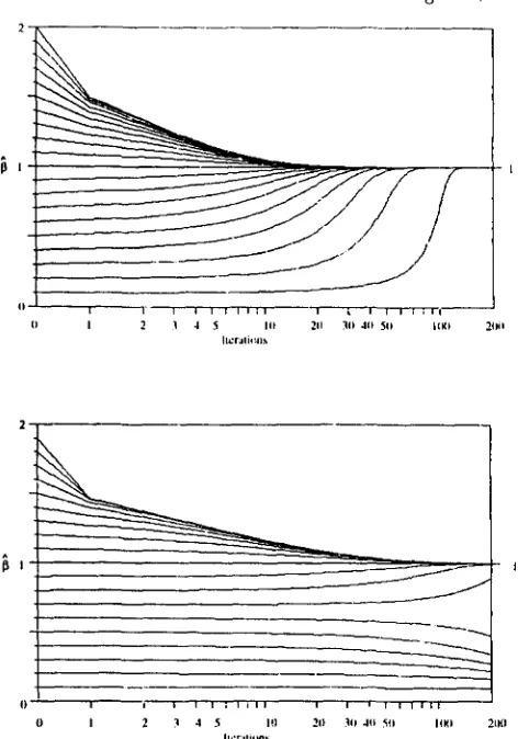
FIGURE 4.-Results from estimation of major gene effect, 8, in a

haploid organism using deterministic sampling of data from the normal distribution. The true value of @ is 1 and total phenotypic variance is 1. Estimates of @ are plotted against iteration number. Starting prior values ranging from 0.1 to 2.0 are shown. For the top graph, the frequency of the major gene is P = 0.1, and in the bottom graph P = 0.5 (assumed known in both cases). Convergence at P = 0.5 was slower, and was not reached for starting values outside a range between about 0.6 to 1.9.

effects and P 2 were then estimated fitting model 6

as described previously, but with the term Za*

dropped.

This procedure was repeated for yfficient itera- tions to achieve convergence in 61 and 02, if successful.

Figure 4 shows some results for an haploid organism where

P

= 1, and Figure 5 shows some results for a diploid organism with

PI

= 1.5 and

&

= 2.0.

T h e results from these deterministic sampling sim- ulations show convergence to exact true @ values in most cases, when true gene frequency is known. How- ever, gene frequency can be estimated at each itera- tion using the counting method of HoEscHELE (1 988),

and for appropriate starting values, this results in convergence at exact true gene frequencies as well as true genotype effects (B. P. KINCHORN and M. J.

MACKINNON, unpublished). These results illustrate that the present approach to estimating

P

values from phenotypes has a rational basis.

Stochastic simulation: T o test the procedure more

7

"

"

-

1

2.0

1.5

I 1 I 2 1 -I r 111 ?II 711 JII (11 IIEI :In\

I ! L W l , W .

FIGURE 5.-Results from estimation of major gene effect, 8, in a

diploid organism using deterministic sampling of data from the normal distribution. The true values of 81 and 8 2 are 1.5 and 2.0,

total phenotypic variance is 1 and true gene frequency of P = 0.5 was assumed known. Estimates of 81 and 8 2 are plotted against

iteration number for two separate runs. Starting prior values for 81

and 8 2 were 0.4 and 0.8 in one run and 0.1 and 2.3 in the other run.

completely, a program was written to simulate multi- generation populations of animals, with recording of pedigree and phenotypes for a single trait.

Breeding values and environmental deviations were separately sampled from appropriate normal distri- butions in the foundation generation. However, to allow for the behaviour of polygenic effects, breeding values and inbreeding coefficients of parents were accommodated in the generation of individuals' breeding values in subsequent generations.

A single locus was also simulated, with two alleles segregating. T h e genotype status of foundation ani- mals were derived through the sampling of gene status at each allelic site from a binary distribution. For animals with known parents, genotype status was de- rived according to the principles of Mendelian segre- gation. For these simulations, major gene effects were set high and gene frequencies set close to intermediate in order to give clearer results from the relatively small data sets used.

01

and

P2

in the absence of polygenic effects: Table 1 shows the estimates of one and two copies of the major gene, with heritability within major genotype class set to zero. Thus breeding values of animals were not fitted. Convergence was achieved in all 50 runs, and estimates were the same when different starting values for

p1

and $2 were used within each replicate popula-

tion. T h e average value of

PI

and

&

over 100 repli- cates (1.445 and 1.892 with standard deviations of 0.251 and 0.273 respectively) compared favourably with the true effects used in data generation (1.5 and

TABLE 1

Estimates of genotype effects 81 and 82 from the first 10 stochastic simulations

Population

8,

(B, = 1.5) 8 2 ( B s = 2.0)

81

(81 = 0) 8 2 (Bn = 0)

1 1.68 2.04 -0.01 0.00

2 1.72 1.46 0.89 0.58

3 1.48 2.17 0.27 0.66

4 1.35 1.96 -0.01 0.01

5 1.63 2.00 0.00 0.00

6 1.28 1.42 0.00 0.00

7 1.80 1.66 0.00 0.00

8 I .38 2.09 0.27 0.90

9 1.33 2.20 0.36 1.16

10 1.29 1.90 1.57 0.60

The simulated data sets consisted of 600 animals each-5 discrete generations of 10 sires mated to 3 dams each, yielding 4 progeny per dam. True genotype effects were =1.5 and 8 2 = 2.0. Other parameters are u = 1, h2 = 0 for polygenic effects and p = 0.5, the latter two assumed known. One round of use of information from relatives was used in calculating genotype probabilities at each iteration. The stopping criterion for convergence was that neither 8, or O2 changed by more than 0.001, and this was achieved by between 17 an+ 105 iterations for the 50 runs tested. Five starting sets of 8, and 8 2 were used [(0.1, 0.2), (0.2, 0.3), (0.5, 0.8). (1.0,

1.5), (2.0, 2.5)l-for each of the replicate populations tested. Within each-replicate, each starting set converged to the same values of @I

and &, and these are shown in the table. Mean values of 81 and 8 2

over the 10 replicates are 1.445 and 1.892 with standard deviations of 0.375 and 0.134 respectively. An additional set of runs was carried out with true genotypic effects set to zero.

cycles generally cause abuse of information from rel- atives if current values of

8,

and 8 2 are considerably

wrong, as can be the case in early iterations.

When true genotypic effects were set to zero, the estimated genotypic effects were either very close to zero, or some significant distance from zero (Table 1). Inspection showed that the errored results came from populations with more platykurtic distributions. Using a second cycle of information from relatives removed some of the apparent dependency of the results on population distribution. For example, the most errored estimates of genotype effects, from pop- ulation 10, changed from (1.57, 0.60) to (0.46, 0.26)

with use of a second cycle of use of information from relatives for calculating genotype probabilities.

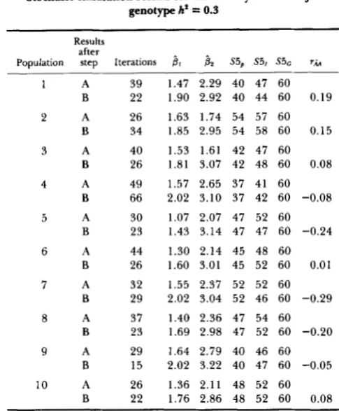
4 1 and P 2 when polygenic effects are involved: Table 2

shows simulation results for heritability within major genotype equal to 0.3. One cycle of use of information from relatives was used in iterations using regressions not fitting polygenic breeding values (step A). How- ever, four cycles of use of information from relatives were used in iterations fitting full regressions (step B), this being of benefit as values of

p1

and

p2

came sufficiently close_to true values after step A.

After step A, P 2 seemed to be biased upwards due

to polygenic effects. Moreover, after step B, the situ- ation was worse, with both

pl

and 6 2 biased upwards,

averaging 1.79 and 3.04 over 100 replicates. This pattern was maintained when only one cycle of use of

TABLE 2

Stochasic simulation results for heritability within major genotype h' = 0.3

1 A 39

B 22

2 A 26

B 34

3 A 40

B 26

4 A 49

B 66

5 A 30

B 23

6 A 44

B 26

7 A 32

B 29

8 A 37

B 23

9 A 29

B 15

10 A 26

B 22

1.47 2.29 40 47 60 1.90 2.92 40 44 60

1.63 1.74 54 57 60 1.85 2.95 54 58 60

1.53 1.61 42 47 60 1.81 3.07 42 48 60

1.57 2.65 37 41 60 2.02 3.10 37 42 60

1.07 2.07 47 52 60 1.43 3.14 47 47 60

1.30 2.14 45 48 60 1.60 3.01 45 52 60

1.55 2.37 52 52 60

2.02 3.04 52 46 60

1.40 2.36 47 54 60 1.69 2.98 47 52 60

1.64 2.79 40 46 60 2.02 3.22 40 47 60

1.36 2.1 1 48 52 60 1.76 2.86 48 52 60

0.19 0.15 0.08 -0.08 -0.24 0.01 -0.29 -0.20 -0.05 0.08

Ten replicate populations were generated. For each population results are given following step A (regressions not fitting animal polygenic breeding values) and step B (follow-up BLUP regressions fitting animal polygenic breeding values). Values of parameters are as for Table 1 , except that h2 = 0.3 for polygenic effects, and there were four cycles of use of information from relatives for genotype probability calculations during step B. S5, is the number of major genes captured when selecting the top 5% of the population on phenotype. S51 relates to screening on an index of genotype prob- abllities [prob(one gene carried)

+

2 X prob(two genes carried)] and S5G relates to screening on true genotype, the latter as an asymptotic control. S ~ C = 60 in all cases as, with P = 0.5, all 5% of animals (30

in number) were invariably homozygous for the major gene. The correlation r h is between estimated breeding value and true breed- ing value for polygenic effects.

information from relatives was used in calculating genotype probabilities, or after intervention to set X

= 1 and X = 5 (instead of the calculated value of X =

2.333) in two additional sets of runs. However, mak- ing no use of information from relatives when calcu- lating genotype probabilities resulted in reduced bias in estimates of genotype effects after step B: true values of 1.5 and 2.0 gave average estimates of 1.527 and 2.538 over 100 replicates.

“”

3 Proportion u i populrtian pcrccncd I

FIGURE 6.-An illustration of the method used to describe screening efficiency,

rx,

in simulations with true genotype status

known. The population is ranked on screening criterion X , and the

cumulative number of major genes captured plotted against number of animals screened. r x = 100 (Ax

-

l)/(Ac

-

l ) , where AX is the area under the curve for screening on criterion X divided by the area for screening on phenotype, and Ac is for screening on true genotype. This gives a scale for r x on which screening on X =

phenotype has a value of 0, and screening on X = true genotypic

status has a value of 100.

genotypic effects iterated towards zero, but with ap- parent tendency to singularity of the mixed model coefficient matrix indicated by increasing numbers of Gauss-Seidel iterations required at each BLUP analy- sis. These results indicate some potential for the de- velopment of strategies or tests to help guard against false positive indication of major gene preseye.

As expected, given the poor estimation of and f i 2

after step B in Table 2, the effectiveness of screening was greater after step A alone. Screening 5% of the population on an index of genotype probabilities [prob(one gene carried)

+

2

x

prob(two genes car- ried)] captured more genes than phenotypic screen- ing-a total of 496 genes captured across the 10 pop- ulations, compared to 452 for screening on phenotype and 600 for screening on true genotype. It should be noted that, with the large genotype effects and inter- mediate gene frequencies used here, phenotypic screening is generally effective, and screening on an index of genotype probabilities is likely to be of less additional value than with other situations.

The effect

of

incorrect prior for gene frequency: Figure 6 describes I?,, a measure of efficiency of screening for major genes on criterion X . This gives a scale for

rx

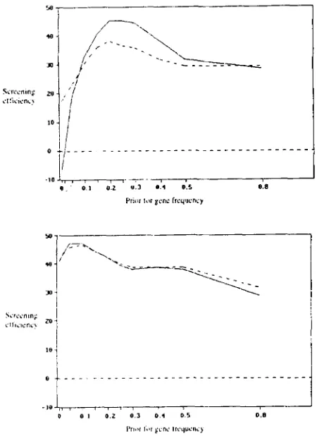
on which screening on phenotype has a value of 0, and screening on true genotypic status has a value of 100. Figure

7

shows the effect of the prior choice of gene frequency on screening efficiency rx. These results suggest that the consequences of either using an incorrect fixed prior for gene frequency or arriving at an incorrect converged estimate are not particularly adverse where true gene frequency is low.

DISCUSSION

This paper has shown some results from use of the method proposed for screening for genes of major effect. T h e approach of deterministic sampling simu-

lation was developed and used to test the method because it gives the properties of an infinite popula- tion but with finite computational requirements. This means that results have no sampling error, and nu-

merical evaluation of, for example, covariances of model terms, can aid diagnosis in theory development. In the present case, these simulations lead to perfect estimation of genotype effects in the absence of poly- genic effects, showing that the method for estimation of major gene effects has a rational basis.

Under stochastic simulation, good estimates of ma- j o r gene effects were obtained in the absence of polygenic effects. However, in the presence of poly- genic effects, upwardly biased estimates of major gen- otype effects resulted when polygenic effects were accounted for, and this reduced the efficiency of screening. This bias was reduced by not using infor- mation from relatives when calculating genotype probabilities. This supports the point made by HOFER

and KENNEDY (1 993), that the correction factors in W

treat each animal equally, despite differing amounts of information contributing to each animal’s genotype probabilities-leading to the case for finding a gener- alised equivalent of W.

Equation 6 suggests that estimates of fixed effects and breeding values may be biased. Deterministic sampling simulation has shown that f

*

can converge to exact true values o f f , even where fixed effects are not orthogonal with major genotype effects (B. P.

KINCHORN and M . J. MACKINNON, unpublished). However, these simulations generate populations of unrelated animals, such that, as for major gene effects, bias in fixed effect and breeding value estimates may result when genotype probabilities are calculated using information from relatives.

Thus further development is warranted to ensure unbiased estimation of f and a, as well as

8.

Finding generalised equivalents of

Vx,

V, and therefore W

may solve these problems. A further step of possible value is to expand

Vx

to include (co)variance among the coefficients in X, F and Z and expand

V,

to include (co)variance among true genotype status and the coefficients in F and Z. This is a logical extension from the current treatment of genotype effects alone to cover all effects in the model.

o /

- 0 l 0 I O 0 . 2 L 0 . 3 I 0 . 4 I 0.5 I 0.8

.i

I ’ m , I<Tg‘.”L‘ Iri’q”cnr)

FIGURE 7.-The effect of choice of prior for gene frequency on

efficiency of screening. Screening efficiency is plotted vertically on a scale on which screening on phenotype has a value of 0, and screening on true genotypic status has a value of 100. The prior for gene frequency is on the horizontal scale. The upper (lower) graph relates to a population with true gene frequency of 0.25 (0.1). Results on the solid line come from using four rounds of use of information from relatives at each iteration, and results on the broken line come from using just one round of use of information from relatives at each iteration. All other parameters are as for Table 1.

This is analogous to the increased relative value of

selection on best linear unbiased predictions of esti- mated breeding value when heritability is decreased.

Although the method seems to be moderately ro- bust to incorrect choice of prior for gene frequency,

it would be desirable to estimate gene frequency from the data. This can be done for maximum likelihood methods (HOESHELE 1988; KNOTT, HALEY and

THOMPSON 199 la,b; HOFER and KENNEDY 1993) and has in fact been added as an extra step in the current method (HOFER and KENNEDY 1993). When estimat- ing gene frequencies in deterministically simulated data, the present approach has resulted in conver- gence at exact true values (B. P. KINCHORN and M. J.

MACKINNON, unpublished).

A number of test statistics have been developed to indicate segregation of a major gene without allocat- ing genotype probabilities. LE ROY and ELSEN (1 992), compare the performance of 22 of these. Many are

based on the properties of distributions, and are likely to be severely affected by skewness and kurtosis of residual effects. T h e same is likely to be true of tnethods which allocate genotype probabilities, espe- cially methods which make use of mixture distribution approaches or contrast within-family variances.

Application: Using these methods for detection of

major genes in individuals may be of little value. Detecting “quantitative trait loci” with the aid of ge- netic markers is not easy-so without the aid of ge- netic markers it should be very difficult. However, as many genes of major effect have been found through simple visual inspection of data, computer assisted methods should be able to do a better. job. Thus, the main value of the current method and its peers prob- ably lies in screening populations for suitable candi- dates to be used either in:

properly designed test matings for detection of ma-

single trait selection lines aimed at developing spe- jor genes with the aid of genetic markers, or

cial genetic resources.

T h e method of HOESCHELE (1988) has appeal and may be more reliable for some applications. The need

to develop likelihood equations algebraically tailored

to the structure of the prevailing data can make its

application difficult. It tends to underestimate major gene effects whereas the current method as presented here tends to overestimate them in the presence of sizable polygenic effects. This is confirmed in recent work by HOFER and KENNEDY (1993) who compare both these methods to their approximated nlaximum likelihood method using simulations of 2-generation pedigrees.

We thank a number of colleagues for useful suggestions, and a referee for providing a proof that E ( y e ) = 0 for haploids, resulting in clearer presentation. Partial funding for this project was provided by the Natural Sciences and Engineering Research Council of Canadd.

LITERATURE CITED

~ O C H R A N , W. G., 1968 Errors of measurement in statistics. Tech-

nometrics 1 0 637-666.

GOLDBERGER, A. S . , 1964 Econometric Theory. John Wiley & Sons, New York.

HOESCHELE, I . , 1988 Genetic evaluation with data presenting

evidence of mixed major gene and polygenic inheritance. Theor. Appl. Genet. 76: 81-92.

HOFER, A., and B. W. KENNEDY, 1993 Genetic evaluation for a

quantitative trait controlled by polygenes and a major locus with genotypes not or only partly known. Genet. Sel. Evol. (in press).

JANSS, L. L. G.,J. H . J . V A N DER WERF andJ. A . M . VAN ARENDONK,

data with an application to FP and Fs crosses. Genet. Sei. Evol. LE Roy, P., and J. M. ELSEN, 1992 Simple test statistics for major

(in press). gene detection: a numerical comparison. Theor. Appl. Genet.

segregation analysis for animal breeding data: a comparison of VAN A R E N ~ N K , J , A. M,,

c,

S M I ~ ~ and B,

w,

KENNEDY,

power. Heredity 68: 299-3 I 1. 1989 Method to estimate genotype probabilities at individual

segregation analysis for animal breeding data: parameter esti-

mates. Heredity 68: 3 13-320. Communicating editor: B. S . WEIR

KNOTT, S. A., C . S. HALEY and R. THOMPSON, 1991a Methods of 83: 635-644.