Quantifying Shared Information Value in a Supply Chain Using Decentralized Markov Decision Processes with Restricted Observations

Abstract

WEI, WENBIN. Quantifying Shared Information Value in a Supply Chain Using Decentralized Markov Decision Processes with Restricted Observations.

(Under the direction of Dr. Russell E. King and Dr. Thom J. Hodgson)

Information sharing in a two-stage and three-stage supply chain is studied. Assuming the customer demand distribution is known along the supply chain, the

information to be shared is the inventory level of each supply chain member. In order to study the value of shared information, the supply chain is examined under different information sharing schemes. A Markov decision process (MDP) approach is used to model the supply chain, and the optimal policy given each scheme is determined. By comparing these schemes, the value of shared information can be quantified. Since the optimal policy maximizes the total profit within a supply chain, allocation of the profit among supply chain members, or transfer cost/price negotiation, is also discussed.

The information sharing schemes include full information sharing, partial information sharing and no information sharing. In the case of full information sharing, the supply chain problem is modeled as a single agent Markov decision process with complete observations (a traditional MDP) which can be solved based on the policy iteration method of Howard (1960). In the case of partial information sharing or no information sharing, the supply chain problem is modeled as a decentralized Markov decision process with restricted observations (DEC-ROMDP). Each agent may have complete observation of the process, or may have only restricted observation of the process. In order to solve the DEC-ROMDP, an evolutionary coordination algorithm is

introduced, which proves to be effective if coupled with policy perturbation and multiple

Biography

Acknowledgements

I cordially thank my co-advisors, Dr. King and Dr. Hodgson. Their consistent support and patient guidance will be treasured for good. My special thank to my

colleague Lauren Davis, whose dissertation research was closely related with mine. We spent plenty of time sharing programming codes and exchanging research insights. I also thank my colleague Kent Marshall, a robot expert, who has brought much joy to me.

I owe many thanks to my Mom, my Dad and my brother for their love and encouragement during so many years.

Table of Contents

List of Figures

... vi

List of Tables

... vii

Chapter 1 Overview

... 1

1.1 Introduction... 1

1.2 References... 3

Chapter 2 Markov Decision Processes with Restricted Observations

5

2.2 Mathematical Model for a ROMDP ... 7

2.2.1 ROMDP Notation... 7

2.2.2 LP Model for a MDP Problem ... 8

2.2.3 NLP Model for a ROMDP Problem... 9

2.3 Methodology for Solving a ROMDP... 11

2.4 Perturbation... 15

2.4.1 Policy Perturbation... 15

2.4.2 Pi Perturbation... 16

2.5 Experimentation... 17

2.5.1 Generic Problem... 17

2.5.2 Supply Chain Problem ... 18

2.6 Conclusion ... 21

2.7 References... 21

Chapter 3 Decentralized Markov Decision Processes with Restricted

Observations

... 23

3.1 Introduction... 23

3.2 Model ... 25

3.2.1 Single agent MDP and ROMDP ... 25

3.2.2 DEC-ROMDP (Multi-agent)... 26

3.3 DEC-ROMDP Algorithm ... 28

3.4 Case Study: A Two-Agent DEC-ROMDP problem... 30

3.4.1 General two-agent DEC-ROMDP Models... 30

3.4.2 DEC-ROMDP Application to a Supply Chain Problem ... 34

3.5 Conclusion ... 38

3.6 References... 38

Chapter 4 Quantifying the Value of Information and Transfer Price

Negotiation in a Supply Chain

... 40

4.1 Introduction... 40

4.1.1 Background ... 40

4.1.2 Literature Review... 41

4.2 Information sharing in a 2-stage Supply Chain ... 42

4.2.1 Modeling ... 42

4.2.1.1 Assumptions ... 42

4.2.1.3 Markov Decision Process Approach ... 43

4.2.1.4 Information Flows ... 44

4.2.2 Methodology ... 46

4.2.3 Experimentation ... 47

4.2.3.1 Design of Experiments I ... 48

4.2.3.2 Design of Experiments II... 50

4.3 Information sharing in a 3-stage Supply Chain ... 51

4.3.1 Modeling and Methodology ... 51

4.3.2 Experimentation ... 53

4.3.2.1 Design of Experiments III ... 53

4.3.2.2 Design of Experiments IV ... 54

4.4 Transfer Cost Negotiation... 55

4.4.1 Determination of Transfer Cost in a 2-stage Supply Chain ... 56

4.4.2 Determination of Transfer Cost in a 3-Stage Supply Chain... 59

4.5 Conclusion ... 63

4.6 References... 63

4.7 Appendix... 65

Chapter 5 Summary and Future Research

... 70

5.1 Summary and Future Research ... 70

List of Figures

Figure 2.1: the percentage of problems solved optimally (Supply Chain ROMDP) ... 20

Figure 2.2: The Average error of Problems Unsolved Optimally (Supply Chain ROMDP) ... 20

Figure 2.3: Max Error of Problems Unsolved Optimally (Supply Chain ROMDP) ... 21

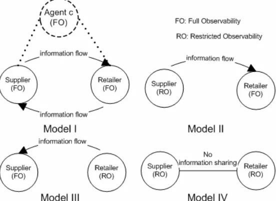
Figure 3.1: General Two-Agent DEC-ROMDP Models with Different Observations .... 30

Figure 3.2: Performance for the General Model I Starting with a Joint Myopic Policy... 31

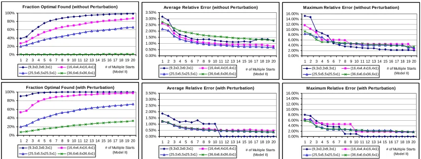
Figure 3.3: Performance for General Model II with Multiple Starts ... 33

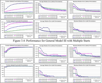
Figure 3.4: Performance for General Model III with Multiple Starts... 34

Figure 3.5: Performance for General Model IV with Multiple Starts... 34

Figure 3.6: Different Information Sharing Schemes for Supply Chain Problems... 37

Figure 3.7: Solving Supply Chain Problems with Multiple Starts and Perturbation... 37

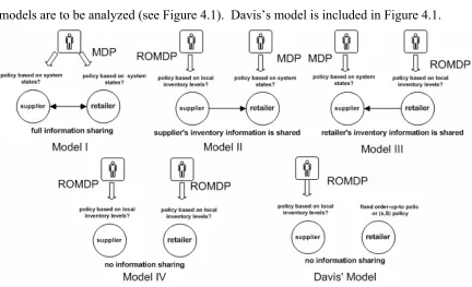
Figure 4.1: Information Flow in Each Model ... 45

Figure 4.2: Relative Information Value when Mean Demand = 5 ... 49

Figure 4.3: g3 and g4 vs. Cs, with Mean Demand = 5 and Cov = 0.3 ... 49

Figure 4.4: Information Flow in Each 3-Stage Model... 52

Figure 4.5: RIVs for the First 32 Problems in DOE3 (all holding costs = 1) ... 53

Figure 4.6: RIV3 Changes with Cm, Cs and Cov... 55

Figure 4.7: Transfer cost between supplier and retailer when CI = 0... 57

Figure 4.8: Transfer cost between supplier and retailer, when CI is charged to the supplier ... 58

Figure 4.9: Profit Triangles before Information Sharing... 61

List of Tables

Table 2.1: Percentage of Problems Solved Optimally (Generic ROMDP) ... 18

Table 2.2: Average error of Problems Not Solved Optimally (Generic ROMDP)... 18

Table 2.3: Max Error of Problems Not solved Optimally (Generic ROMDP)... 18

Table 2.4: Average Execution Time (seconds) (Generic ROMDP) ... 18

Table 3.1: Average Execution Time (Seconds) (General Model I) ... 32

Table 4.1: Design of Experiments I ... 48

Table 4.2: Design of Experiments II... 50

Table 4.3: Design of Experiments III ... 53

Table 4.4: Summary of Mean Comparison for RIVs... 53

Table 4.5: Design of Experiments IV ... 54

Table 4.6: Worthy Curve Analysis for 96 Problem Instances in DOE2 when CI=0... 65

Chapter 1 Overview

1.1 Introduction

If information in a supply chain is not shared among the individual chain elements (e.g., demand information), actual demand information (from downstream to upstream of the supply chain) may be distorted (this is also termed the bullwhip effect, Lee et al. 1997) and cause unnecessary cost. It has been reported that information sharing is beneficial to a supply chain, especially in reducing the bullwhip effect (Lee et al. 1997, 2000, Cachon and Fisher 2000) and supply chain cost (Gavirneni et al. 1999,

Swaminathan et al. 1997, Tan 1999). However, it may not be beneficial to a supply chain if the cost of adopting the inter-organizational information system is too high

(Swaminathan et al. 1997, Cohen 2000). In terms of information sharing, the concern is usually which production information to share and how to share it to maximize the mutual benefits in a supply chain (Huang et al. 2003).

The objective of this dissertation is to quantify the value of sharing inventory information in a make-to-stock environment and optimize the operational control for a two-stage and three-stage supply chain through appropriate information sharing. This dissertation is an extension of Davis’ (2004) work on a two-stage supply chain with a single capacitated supplier and a single retailer. Davis finds the supplier’s optimal policy by assuming the retailer uses a fixed policy, such as a base stock policy or (s, S) policy. Davis’ work has some limitations. First, the retailer’s policy is fixed. A more flexible policy could possibly achieve better system performance. Second, only the value of sharing retailer’s inventory information is examined. This dissertation allows the retailer to use a flexible policy, and examines the value of sharing suppliers’ inventory

information. However, the problem becomes much more complicated since the suppliers and retailer need coordination when making their replenishment decisions in order to optimize the supply chain. Four different information sharing models are examined in a two-stage supply chain problem, while eight different models are examined in a three-stage supply chain.

multi-echelon inventory system, researchers usually assert that a certain type of policy, like a base-stock policy, is optimal for one stage (Gavirneni et al. 1999, Gavirneni 2002, Simchi-Levi and Zhao 2002ab, Davis 2004) or both stages (Lee et al. 2000), and then find the specific policy for each stage. Those assumptions do not pursue system-wide optimality, since the assertion comes from the results of a single-stage inventory system, and the possibility of coordination between members is ignored. To overcome this drawback, we model a multi-stage supply chain as a Markov Decision Process (MDP).

In the context of a MDP, an agent with full observation (due to information sharing) actually faces a common MDP problem (also called a completely observable MDP, COMDP), while an agent with restricted observations (lack of information

sharing) faces a MDP with restricted observations (called ROMDP). Davis (2004) solves a single agent ROMDP. As an extension, this dissertation provides a solution for multi-agent (decentralized) MDP or ROMDP problems (called DEC-ROMDP), where supply chain members need to be coordinated in order to maximize profit.

This dissertation proposes and analyzes an infinite horizon ROMDP with an average cost criterion, with an objective to maximize the average reward. A

computationally efficient algorithm is developed to find optimal policies based on the policy iteration method of Howard (1960) for the infinite horizon undiscounted cost case. Formally, a ROMDP can be represented as a mixed integer nonlinear programming (MINLP) problem, for which it is difficult to find the global optimal solution. The basic heuristic proposed here includes two steps: value determination and policy improvement. It is proven that the policy improvement searches for an optimal solution by following a steepest ascent direction. We also propose perturbation methods, such as policy

perturbation and Π perturbation (Π is the system steady state probability vector), to improve local optima towards a global optimal policy. Successive approximation is used to reduce computational effort. In addition, Ding’s encapsulation evolution method (1985) can be used to further reduce computational effort for specially structured supply chain problems (Davis 2004).

decision problem (MTDP) (Pynadath and Tambe, 2002). An evolutionary coordination algorithm is used to make a joint policy evolve to a locally optimal solution, and then perturbation methods and a multiple restart strategy are used to improve the policy. By using the tools for solving DEC-ROMDP models, a wide range of supply chain problems with different information sharing schemes are solved.

Chapter 2 proposes the mathematical model for an infinite horizon ROMDP with an average cost criterion and introduces heuristic algorithms for solution. Chapter 3 gives the definition of DEC-ROMDP and proposes an evolutionary coordination

algorithm to solve the multi-agent decision problems. Chapter 4 applies the evolutionary coordination algorithm to two-stage and three stage supply chain problems, and

elaborates on information sharing and transfer cost negotiation within the supply chain. Chapter 5 outlines the future research to be performed.

1.2 References

Bernstein, D., S. Zilberstein, and N. Immerman, 2000. The complexity of decentralized

control of MDPs. In Proceedings of the Sixteenth Conference on Uncertainty in Artificial

Intelligence.

Cachon, G.P., and M. Fisher. 2000. Supply chain inventory management and the value of shared information. Management Science, 45, 843-856.

Cohen, S.L. 2000. Asymmetric information in vendor managed inventory systems. PhD Thesis, Stanford University.

Davis, L.B., 2004, State Clustering in Markov Decisions Processes with an Application in Information Sharing, unpublished Ph.D. dissertation, Industrial Engineering

Department, N.C. State University.

Ding, F.Y., T. Hodgson and R. King, 1988. A methodology for computation reduction for specially structured large scale Markov decision problems. European Journal of

Operational Research. Volume 34:105-112.

Gavirneni, S., R. Kapuscin, and S. Tayur. 1999. Value of information in capacitated supply chains. Management Science, 46, no.1: 16-24.

Gavirneni, S. 2002. Information flows in capacitated supply chains with fixed ordering cost. Management Science, 48, 644-651.

Howard, R. 1960. Dynamic Programming and Markov Processes. MIT Press,

Cambridge, MA

Huang, G.Q., J.S.K. Lau, and K.L. Mak. 2003. The impacts of sharing production

information on supply chain dynamics: a review of the literature. International Journal of

Lee, H., Padmanabhan, V. and Whang, S. 1997. Information distortion in a supply chain: the bullwhip effect. Management Science, 43, 546-558

Lee, H.L., K.C. So, and C.S. Tang. 2000. The value of information sharing in a two-level supply chain. Management Science, 46, 626-643.

Pynadath, D., and M. Tambe, 2002. The communicative multiagent team decision

problem: Analyzing teamwork theories and models. Journal of Artificial Intelligence

Research, 16, 389-423.

Simchi-Levi, D., and Y. Zhao. 2002a. The value of information sharing in a two-stage supply chain with production capacity constraints. Working paper, Northwestern University, Evanston, IL.

________________________. 2002b. The value of information sharing in a two-stage supply chain with production capacity constraints: the infinite horizon case.

Manufacturing and Service Operations Management, 4, no.1: 21-24.

Chapter 2 Markov Decision Processes with Restricted

Observations

2.1 Introduction

This chapter presents a computationally efficient procedure to determine control policies1 for an infinite horizon, undiscounted Markov decision process (MDP) with restricted observations (ROMDP). In the MDP framework, it is usually assumed that an agent interacts synchronously with a world (Kaelbling, Littman, and Cassandra 1998). A Markov decision process can be defined as a tuple < S, A, T, R >. S is a finite set of |S|

world states; A isa set of |A| actions; T: S ×A ×S → [0, 1] is the state-transition model,

where T(s, a, s’) represents the probability of transition from state s to s’, given that the

agent takes action a; R: S × A→R is the reward model, where R(s, a)represents the

expected reward for taking action a in state s (assumed to be bounded in this chapter). In

a common MDP, the world state is assumed as completely observable to the agent, so this process is also called COMDP (completely observable Markov decision process) in this dissertation. Since this process is considered observable and the state of the system is observable to the agent, the stationary policy is a function of the state space.

If the world state is not completely observable to the agent, this process is a partially observable Markov decision process (POMDP), which can be defined as a tuple

<S, A, T, R, Z, O>, where S, A, T, and R are the same as those in a COMDP. Z is a finite

set of |Z| observations; O: S×A×Z→[0, 1] is the observation probability distribution

model, where O (z, a, s’) represents the probability that the agent observes z given that it

took action a and then the world state reached s’. As the agent cannot observe the state

directly, a POMDP policy, different from a COMDP policy, is not a function of the state space, but the function of belief states, i.e., the steady state probability distribution. Since the belief state is continuous, it is not realistic to find a policy based upon every possible belief state. However, an optimal policy can be based only upon finite partitions of belief

1 _{This dissertation attempts to find the optimal stationary deterministic policy for an infinite horizon}

state space (Smallwood and Sondik 1973)2. Several algorithms have been developed to efficiently determine the partitions (Sondik 1971, Cheng 1988, Littman 1994, and Zhang and Liu 1996).

A Markov decision process with restricted observation is a special POMDP, and it can be represented by a tuple < S, A, T, R, Z, G >, where S, A, T, R,and Z are the same as

those in a POMDP. G: S → Z represents the mapping function from a state to a single

observation for the agent. If a state s outputs an observation z, it can be denoted as G(s)

=z. A ROMDP policy is represented as a function of the observation space. In this

policy, if an action a is applied given an observation z, this action a would apply to any

possible state s satisfying G(s) = z, that is, the action a must be implementable/admissible

to all these states. Hence, a ROMDP policy is also called an “implementable policy” (Serin and Kulkarni 1995) or “admissible policy” (Smith 1971).

Although an ROMDP is a special POMDP, it is still intractable to solve. Serin and Kulkarni (1995) develop an algorithm that finds local optimal stationary randomized policies for the infinite horizon discounted reward case, with the objective to optimize the total discounted reward. Serin and Avsar (1997) introduce a similar algorithm for the finite horizon discounted reward case, and prove a deterministic optimal policy exists in this case. Smith (1971), Hordijk and Loeve (1994), and Hastings and Sadjadi (1979) present algorithms that determine deterministic policies for infinite horizon undiscounted reward problems, with the objective to optimize the average reward. The algorithm developed by Hastings and Sadjadi (1979) is enumerative based and thus intractable for large problems. The algorithm developed by Smith (1971) is a policy iteration type of algorithm containing enumerative component when a better policy cannot be determined. None of the above algorithms have addressed to an infinite horizon large scale ROMDP problem. This chapter introduces a computationally efficient algorithm that also finds optimal deterministic policies, based on the policy iteration method developed by Howard (1960) for the infinite horizon undiscounted cost case. This chapter

demonstrates empirically that the algorithm finds the optimal deterministic policy for over 99% of the general ROMDP problem instances generated. In the instances where the optimal policy cannot be determined, the average error in the objective function is

less than 1%. This algorithm achieves better performance for supply chain ROMDP problems.

2.2 Mathematical Model for a ROMDP

2.2.1 ROMDP Notation

The process being analyzed is a Markov Decision Process with state space S and action space A. The state of the system cannot be observed, however some output of the system is observable. Based on those outputs, one can infer the state or possible states of the system. This chapter finds an optimal control policy defined over the observation process that maximizes the long term average reward. The optimal policy has the

property that each state within a given observation set takes the same action. A summary of the problem notation is presented below.

S: The set of possible states {1…N}.

A: Theset of available actions {1…M}.

Xn: A random variable that defines the state at time n.

Yn: A random variable that defines the action by the agent at time n.

a ij

p : The one step transition probability from state i to j given an action a.

} ,

|

{X ₁ j X i Y a P

p_ija = _n+ = _n = _n = ,∀i,j∈S,∀a∈A,

cia: The expected immediate reward associated with transitioning to state i given

action a.

Z: The set of observable outputs{1...K}.

G(i): A function mapping a state i to a single observable output in the set Z.

Sk: A partition of the state space S satisfying {i: G(i) = k}. Without loss of

generality, it is assumed any state space partition has the same number (say L)

of states. Obviously, K*L = N, and Sk ={(k-1)*L+1, (k-1)*L+2…k*L}, k∈Z.

A(k): The set of admissible actions for the observation set Sk. Obviously, A(k) ⊆

A. Without loss of generality, it is assumed A(k) = A for a generic ROMDP.

2.2.2 LP Model for a MDP Problem

Before presenting the mathematical model for a ROMDP with undiscounted reward and infinite horizon, this section starts from the linear programming model (LP) for an underlying common MDP problem (Wolf and Dantzig, 1962).

A a S i x x S i p x x x c ia M a N i ia M a N j a ji ja M a ia M a N i ia ia ∈ ∈ ∀ ≥ = ∈ ∀ =

∑∑

∑∑

∑

∑∑

This primal problem aims to maximize the average reward. Its decision variable

ia

x can be interpreted as the steady state probability that state i will be visited at a typical

transition and action a will be applied. The constraints can be satisfied with some

feasible steady state probabilities associated with a certain randomized stationary policy, that is, a policy that chooses at state i the action a with probability x_ia.

LP theory implies that the optimal solution is always obtained with deterministic

stationary policies. Indeed, if α* is an optimal (deterministic) stationary policy that is uni-chain (α*(i) denotes the action for the state i), and xi* is the corresponding steady

state probability of state i, then

⎩ ⎨ ⎧ = = otherwise. 0 ) ( * if *

* x a i

xia i

α

is an optimal solution of the

primal problem.

It is also insightful to investigate the following dual formulation for the problem.

S j v A a S i c v p v g g j ia N j j a ij i ∈ ∀ ∈ ∈ ∀ ≥ − +

∑

2.2.3 NLP Model for a ROMDP Problem

By adding observability constraints to the above primal MDP problem, the nonlinear programming (NLP) model for a corresponding ROMDP problem is obtained.

Before formulating the NLP model, the following definitions are introduced.

) ,..., | ... | ,..., | ,..., ,

(α₁₁ α₁₂ α₁M α₂₁ α₂M αK₁ αKM

α = _{is a ROMDP policy, in which}

αka denotes the probability that action a is applied given observation k. Here

A a S i x x x x k i ia M a ia ia

ka = = ∀ ∈ ∈

∑

∑

=

, 1

.

The NLP model for the ROMDP is given as

S i x Z k x S i p x x x c i M a ka N i i N j M a a ji a j G j i N i M a a i G i ia ∈ ∀ ≥ ∈ ∀ = = ∈ ∀ =

∑

∑

∑∑

∑∑

1 1 ( )

1 1 ) ( α α α

Let P(α) be the matrix defined with entries pij(α), where

( )

∑

1 ()

α

α ,

and

1 ( ) M

i ka ia a

c α α c

=

=

∑

( )

( )

( )

[

]

∑

∑

The matrix [I-P(α)] is not invertible since it contains a redundant constraint. To

reduce this redundant constraint, replace the Nth column of this matrix with all ones and define an invertible matrix Q(α).

⎥ ⎥ ⎥ ⎥ ⎦ ⎤ ⎢ ⎢ ⎢ ⎢ ⎣ ⎡ − − − − − − = 1 ... ) ( ) ( 1 ... ... ... 1 ... ) ( 1 ) ( 1 ... ) ( ) ( 1 ) ( 2 1 22 21 12 11 α α α α α α α N N p p p p p p Q

Furthermore, define an n-element vector b=(0,0…1).

Then transform the NLP into

( )

( )

∑

By removing the variable x,it becomes

( )

( )

ka = ∀ ∈

= Φ

∑

Note the optimal solution to this NLP problem may be a randomized stationary

policy α. That is,αka, a component of an optimal policy may be a number other than 0

transformed into a mixed integer nonlinear programming problem (MINLP) by adding the integer constraint.

( )

∑

2.3 Methodology for Solving a ROMDP

Definition 1:β =(β₁₁,β₁₂,...,β₁M |β₂₁,...,β₂M |...|βK₁,...,βKM) is a feasible direction at

a feasible policy α if and only if α+θβ is also a feasible policy for some θ>0.

Clearly, k Z

M

a

ka = ∀ ∈

∑

=

, 0 1

β and βka ≥0for αka =0 andβka ≤0for αka =1. Without loss

of generality, the normalization restriction | | 1

1 1 =

∑∑

β is assumed on the feasible

direction (Serin and Kulkarni 1995).

Definition 2: A feasible direction β is an ascent direction at a feasible policy α

ifΦ(α +θβ)>Φ(α), for all θ∈(0,δ) for some δ>0.

Lemma 1: If a feasible direction βsatisfiesthat ∇Φ₍α₎Tβ _{is positive, then} β _{is an ascent}

direction at policy α. Here, ∇Φ(α) is the gradient of the objective function at α.

Proof: It is Obvious according to the definition of the gradient. (Q.E.D)

Theorem 1: Let v =[v₁...vn]be the solution to Q(α)v= c(α),x =[x1...xn] be the solution

to xQ(α)=b, and Pka is the matrix with

⎩ ⎨ ⎧ = ≠ = Otherwise 0 and , ) (

if G i k j N p

p

a ij ka

ij . If

)) ( ( max arg 1 *

∑

∑

k x c p v

a , then β satisfying

⎪ ⎩ ⎪ ⎨ ⎧ ≠ = − = = = otherwise , 0 and , 1 if , 2 / 1 and , 0 if , 2 / 1 * * k k ka ka

ka a a

a a

α α β

is a steepest ascent direction at the current policy α, which maximizes the directional

derivative ∇Φ₍α₎Tβ_.

First derive the gradient of the objective function at α, i.e. ∇Φ(α). To compute

the gradient, it is assumed that the objective function is continuous and differential at

every point of feasible region, i.e., α can be randomized.

( )

( )

_{( )}

( )

( )

_∑

_∑

_{( )}

∑

∑

∑

Let _⎥

⎦ ⎤ ⎢ ⎣ ⎡ ∂ ∂ ∂ ∂ ∂ ∂ = ∂ ∂ ka N ka ka ka x x x x α α α

α 1 , 2 ...

0 ) ( ) ( = ∂ ∂ + ∂ ∂ ka ka Q x Q x α α α α , Define ) ( ) ( ka ka Q P α α ∂ ∂ −

= . Clearly, ka

P is the matrix with

⎩ ⎨ ⎧ = ≠ = Otherwise 0 and , ) (

if G i k j N p p a ij ka ij .

Then ka

ka P x Q x ₌ ∂ ∂ ) (α

α . Since Q(α)−1exists, ∂ = ( )−1

∂ _α

α xP Q

x ka

ka

.

Therefore,

( )

∑

∈ − + = ∂ Φ ∂ k S i ka i ia ka c Q P x x

c (α) 1 (α) α

α

Let v =[v₁...v_n] be the solution to Q(α)v= c(α), Then

( )

_∑

_∑

x (α)

α α

.

In order to find the steepest ascent direction at the current policy α, ∇Φ₍α₎Tβ

should be maximized. Note the current policy α must be deterministic, for instance, if α

uses action b for a state set Sk, there must be

⎩ ⎨ ⎧ = = otherwise , 0 if ,

1 a b

ka

α . It is obvious for a state

0 for

0 =

≥ ka

ka α

β , 1βka ≤0for αka = , and k Z

M

a

ka = ∀ ∈

∑

=

, 0 1

β . In order to

maximize∇Φ₍α₎Tβ_{, it is obvious to choose a component} β

ka* among(βk1,...,βkM),

where * argmax( ( ))

ka A

a

a

α α ∂

Φ ∂ =

∈ , and set βka* to be -βkb, other components zero.

Considering the normalization restriction | | 1

1 1

=

∑∑

= =

K

k M

a ka

β , so βka* = 1/2, and βkb = -1/2. If

a* = b, every component of (βk₁,...,βkM) is zero. (Q.E.D)

If a steepest ascent direction β at a current policy α is zero, the policy α is

considered as a local optimal policy. Otherwise, if βis not zero, there exists a step size

θ>0such thatα+θβ(it might be a randomized policy)is better thanα, i.e.

Φ(α+θβ)>Φ(α). Since αis deterministic and the steepest ascent direction β is defined as

Theorem 1, it is necessary to make θ= 2 such that α’=α+θβ is also deterministic. Note a

step size θ= 2 may not satisfy Φ(α+θβ)>Φ(α). However, it is sufficient to keep this step

size and ensure policy move between deterministic policies. This movement has a

drawback that may not keep Φ(α+θβ)>Φ(α), but if that is a case, the current policy α is

also considered as a local optimal policy. Based on this guidance, a heuristic algorithm is presented below.

Definition 3: If starting from a current policy α, β is the steepest ascent direction found

according to Theorem 1, then the operation of getting a new policy α’=α+2β is called a

policy improvement.

Definition 4: A policy α is a local optimal solution, if after a policy improvement the

policy change from α to α’, and Φ(α')≤Φ(α).

Lemma 2: Let v =[v₁...vN]be the solution to Q(α)v= c(α), then g = vN is the gain

associated with the policy α.

Proof: For a policy α, the gain is g = xc(α), where x is the steady state probability.

Since _{= (α)}−1

Q b

x , the gain is g =bQ(α)−1c(α)=bv. Hence g = vN as b = [0,0, …,1]’.

As deterministic policies are of interest, it is sufficient to only carry the

information needed in terms of the action taken for a given observation set Sk, and this

dispels the necessity to construct a K*M-elementdecision vector α to represent an

implementable policy. Therefore, a K*M-elementoriginal decision vector α can be

represented by K-element policy vector δ =[δ₁...δ_K], where δ_k =a if α_ka =1.

Then Q(α) has entries pij(α) where

( )

),

( ijGi

a

a ij a i G

ij p p

p α =

∑

Similarly, the vector c(α) has entries ci(α) where

( )

_∑

a

i a i G ia

i c c _Gi

c α α _{(), ,δ ()}

These substitutions will be denoted as Q(α/δ)and c(α/δ). To simply notation, a policy is

always considered as K-element vector notation in this chapter, but readers should keep

in mind that the policy can have two representations. Use αk to represent the action used

for observation set k.

Heuristic Algorithm: The algorithm for finding an implementable policy is as below.

Step 0. Initialization

Generate an initial admissible policy α.

Set g* = -∞.

Step 1. Value Determination

Determine relative values v, steady state probabilities x, andthe gain gδ.

x

(a). If gα >g*, set g* = g and proceed to Step 2.

(b) If gα ≤ g*, the current solution is a local maximum, and stop.

Step 2. Policy Improvement

For all k∈ Z find an action

∑

∑

=

∈ +

=

k

S i

N

j

j ka ij ia

i A

a

k x c p v

1

) (

max arg

α , and

go to step 1.

Lemma 3: The algorithm defined above will terminate at a local optimal solution after a

Proof: By assuming the reward for the Markov decision process is bounded, the gain

associated with any policy would be bounded. Since the policy improvement step will not increase the gain indefinitely, there must be a finite number of iterations such that the algorithm terminates. (Q.E.D)

2.4 Perturbation

The above heuristic, called Normal Convergence, does not guarantee to obtain the

global optimum unless only a single local optimum exists. Therefore, the normal convergence is augmented by a local improvement procedure, called perturbation, to

increase the probability of finding the global optimum.

In order to improve the heuristic, this chapter also provides two perturbation

methods. One is called Policy Perturbation, and the other is called ΠPerturbation.

2.4.1 Policy Perturbation

Policy perturbation is carried out based on the policy from Normal Convergence. The basic idea is to perturb the best policy obtained from normal convergence, and form a neighboring policy. By starting from this new policy, repeat value determination and policy improvement cycle. Once a better policy is found, continue perturbing this policy until no better policy can be found.

Obviously, how a policy is perturbed and how many perturbations are performed impacts the effect of policy perturbations. Two approaches for policy perturbation are developed. The first one (denoted as PP1) modifies only one element in the policy vector, and the number of the perturbation increases proportionally to the length of the policy vector. The second one (denoted as PP2) is an extension of the first one. After modifying one element in the policy vector, it tries to modify any adjacent two elements in the policy vector. Obviously, PP2 has more perturbations than PP1.

How to modify the element to obtain a new policy? During the policy

improvement step, the test quantities for different alternatives are computed, and the best alternative is determined, which maximizes the test quantity, say,

∑

∑

=

+

k

S i

N

j

j ka ij ia

i c p v

x

1

)

( . Actually, the second best alternative can serve as the candidate

The original policy α =(α₁₁,α₁₂,...,α₁M |α₂₁,...,α₂M |,...|αK₁,...,αKM) is not

convenient to represent. According to the characteristic of deterministic policy α, this chapter simplifies the representation of this policy with K-element policy vector, of

which each element corresponds to the selected action index for one of the K

observations. For instance, for a ROMDP problem with N = 16, M = 4, K = 4, and L = 4, ,

if a best policy is (4, 3, 3, 2) after Normal Convergence, the original representation of

policy is actually α=(0,0,0,1| 0,0,1,0| 0,0,1,0| 0,1,0,0). Assume the second best

alternatives are (3, 4, 1, 3). Policy Perturbation I (denoted as PP1) results in the following policies after perturbation: (3,3,3,2), (4,4,3,2), (4,3,1,2), and (4,3,3,3). The Policy

Perturbation II (denoted as PP2) results in the following policies after perturbation: (3,3,3,2), (4,4,3,2), (4,3,1,2), (4,3,3,3), (3,4,3,2), (4,4,1,2), (4,3,1,3), and (3,3,3,3). Notice

that the first element and the last element in a vector are treated as adjacent.

2.4.2 Pi Perturbation

PiPerturbation (Π Perturbation) is similar to the policy perturbation, except that

it perturbs a steady state probability vector x instead of a policy vector. Although the

policy is not modified, modification of vector x may lead to a better policy by repeating

the value determination and policy improvement cycle. If a better policy is found, again perturb the vector x associated with this policy. The process is continued until no better

policy can be found.

Unlike a policy vector, vector x has a continuous space. Different from policy

perturbation, Π perturbation is performed by randomizing the x vector under the

expectation that this modified vector x will eventually lead to a better policy during the

value determination and policy improvement cycle.

Two types of Πperturbation are developed (set ε = 1/N).

(1) ΠPerturbation I (denoted as PiP1)

i) xi =xi +ε∀i

ii) i

x x

x _N

i i i

i = ∀

∑

=1

i) ⎩ ⎨ ⎧

∀ > +

∀ ≤ −

=

i r

x

i r

x x

i i i

, 5 . 0 if

, 5 . 0 if ) ,

0 max(

ε ε

,

where r is randomly generated value between 0 and 1.

ii) i

x x

x _N

i i i

i = ∀

∑

=1

2.5 Experimentation

2.5.1 Generic Problem

To evaluate the effectiveness of an algorithm, different sizes of generic ROMDP problems are generated, and each problem has 1000 random instances. The heuristic solution of solving these instances was compared with the optimal solution through brute force enumeration. Let K represent the number of partitions, L the number of states in

each partition, N=K*L the number of total states in the system, and M the size of action

space.

Table 2.1 gives the percentage of problems solved optimally. By applying

Normal Convergence (NC), Policy Perturbation I and II (PP1 and PP2), and Π

Perturbation I and II (PiP1 and PiP2), 88.3%, 98.5%, 99.2%, 98.8%, and 99.1% of 1,000 problem instances are optimally solved, respectively. By combining PP1 and PiP2, 99.7% of 1,000 problem instances were solved optimally.

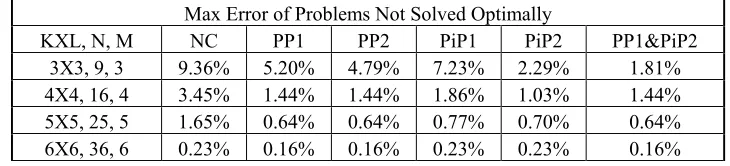
Table 2.2 gives the average error from the optimal solution for those problems that are not solved optimally. Table 2.3 gives the maximum error from the optimal solution for those problems that are not solved optimally. Table 2.4 gives the average execution time (seconds) for each problem. The results show that NC can optimally solve at least 85% of generic ROMDP problems. With policy perturbation or Π

Table 2.1: Percentage of Problems Solved Optimally (Generic ROMDP)

% of Problem Solved Optimally Among 1000 Instances

KXL, N, M Policy space NC PP1 PP2 PiP1 PiP2 PP1&PiP2

3X3, 9, 3 33_{= 27 88.90% 97.40% 98.30% 96.20% 98.10% 98.90%}

4X4, 16, 4 44_{=256 87.60% 98.30% 98.90% 97.70% 98.40% 99.50%}

5X5, 25, 5 55_{= 3125 88.30% 98.50% 99.20% 98.80% 99.10% 99.70%}

6X6, 36, 6 66_{= 46656 98.4% 99.6% 99.7% 98.7% 98.4% 99.6%}

Table 2.2: Average error of Problems Not Solved Optimally (Generic ROMDP)

Average Error of Problems Not Solved Optimally

KXL, N, M NC PP1 PP2 PiP1 PiP2 PP1&PiP2

3X3, 9, 3 1.54% 1.33% 1.18% 1.39% 0.79% 0.68%

4X4, 16, 4 0.69% 0.43% 0.45% 0.57% 0.40% 0.55% 5X5, 25, 5 0.34% 0.19% 0.25% 0.16% 0.21% 0.28% 6X6, 36, 6 0.09% 0.09% 0.09% 0.09% 0.09% 0.09%

Table 2.3: Max Error of Problems Not solved Optimally (Generic ROMDP)

Max Error of Problems Not Solved Optimally

KXL, N, M NC PP1 PP2 PiP1 PiP2 PP1&PiP2

3X3, 9, 3 9.36% 5.20% 4.79% 7.23% 2.29% 1.81%

4X4, 16, 4 3.45% 1.44% 1.44% 1.86% 1.03% 1.44% 5X5, 25, 5 1.65% 0.64% 0.64% 0.77% 0.70% 0.64% 6X6, 36, 6 0.23% 0.16% 0.16% 0.23% 0.23% 0.16%

Table 2.4: Average Execution Time (seconds) (Generic ROMDP)

Average Execution Time (seconds3_{) for 1000 Problem Instances}

KXL, N, M NC PP1 PP2 PiP1 PiP2 PP1&PiP2 Enumeration

3X3, 9, 3 0.00026 0.0013 0.0025 0.0017 0.0024 0.0035 0.0014

4X4, 16, 4 0.0012 0.0063 0.011 0.0083 0.014 0.018 0.037

5X5, 25, 5 0.0030 0.024 0.043 0.037 0.059 0.073 1.5

6X6, 36, 6 0.01 0.08 0.16 0.08 0.23 0.30 74

2.5.2 Supply Chain Problem

The ROMDP algorithm is also applied to a two-stage supply chain ROMDP problem (maximization problem), in which the retailer uses a fixed order-up-to policy, and the supplier aims to optimize the system without knowing the retailer’s inventory information.

The assumptions include: There is a customer demand distribution that retailer must satisfy. The supplier’s production and the retailer’s order shipment are

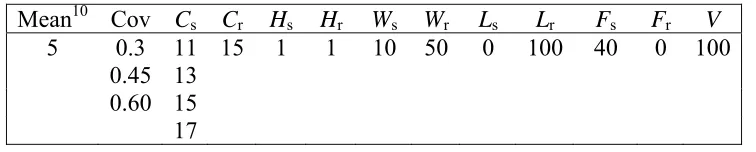
synchronous, and their lead-time is a typical period. Each has a maximum inventory capacity. The supplier’s production capacity is limited by its inventory capacity, since it cannot produce more than can be accommodated in his warehouse. The retailer applies order-up-to policy, and the order-up-to level is its inventory capacity. Note that the excess demand from a customer or the retailer is lost. The cost structure includes production/order setup cost (F_s and F_r), holding cost (H_sand H_r), variable

production/purchase cost (Wsand Wr), and a stock out penalty cost (Ls and Lr). Here

the subscription of “s” stands for the supplier and “r” for the retailer.

The typical parameters for the supply chain are as follows.

s

C :The inventory capacity for the supplier.

r

C :The inventory capacity for the retailer.

V: The selling price to the customer.

d: The demand from the customer, d= 0,1…D, assuming D=Cr.

s

i : The inventory level of the supplier, is =0,1,2,...,Cs. The supplier’s

observation on his own inventory is z_s =i_s.

r

i : The inventory level of the supplier, i_r =0,1,2,...,C_r. The retailer’s observation

on her own inventory is zr =ir.

s

k : The production order quantity placed by the supplier. The possible order

quantity depends on the supplier’s inventory capacity and current inventory level, i.e.,

s s

s C i

k =0,1,2,..., − _.

The objective is to find the optimal policy for the supplier, who only observes his own inventory, such that the supply chain total profit is maximize. Obviously, this is a typical ROMDP problem. The system state can be represented by the inventories of both

the supplier and the retailer, i.e., i=(is −1)∗Cs +ir, and the action can be represented by

the order quantity of the supplier, i.e., ks. Since the supplier has the capacity restriction,

correspondingly isand ir respectively), under an action ks and a customer demand d,

then the total profit of this supply chain would be:

] ) ( * * )) , min( , 1 min( * ) , 1 min( * * * [ ) , min( * ) , , ( + − + + + + + − = r r r s r s s s s r r s s r s i d L F i k F k k W i H i H i d V d k i P

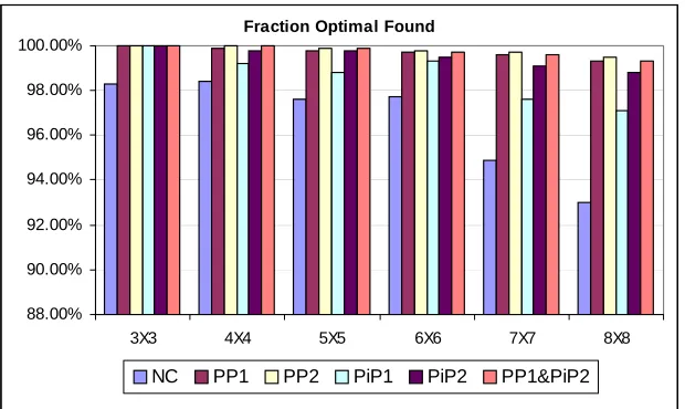
Since C_s and C_r determines the problem size, 1000 problem instances for

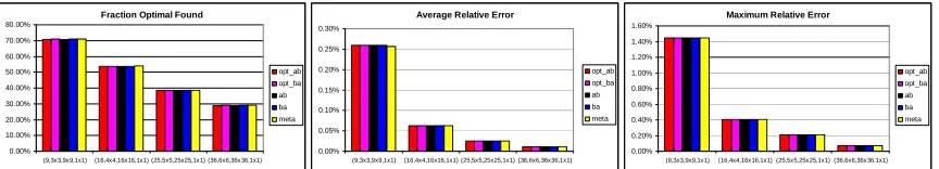
different Cs and Cr are generated. It appears that the performance is better than generic

problems (see Figure 2.1, Figure 2.2, and Figure 2.3). Note that Cs + 1 = K and Cr + 1 =

L. Without any perturbation, NC method has achieved more than 93% of problems solved

optimally. With perturbation, almost solve all the problems are solved; even for those problems that are not solved optimally, the average errors are close to zero.

Fraction Optimal Found

88.00% 90.00% 92.00% 94.00% 96.00% 98.00% 100.00%

3X3 4X4 5X5 6X6 7X7 8X8

NC PP1 PP2 PiP1 PiP2 PP1&PiP2

Figure 2.1: the percentage of problems solved optimally (Supply Chain ROMDP)

Average Relative Error

0.00% 2.00% 4.00% 6.00% 8.00% 10.00% 12.00%

NC PP1 PP2 PiP1 PiP2 PP1&PiP2

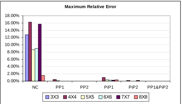
Maximum Relative Error

0.00% 2.00% 4.00% 6.00% 8.00% 10.00% 12.00% 14.00% 16.00% 18.00%

NC PP1 PP2 PiP1 PiP2 PP1&PiP2

3X3 4X4 5X5 6X6 7X7 8X8

Figure 2.3: Max Error of Problems Unsolved Optimally (Supply Chain ROMDP) Table 2.5: Average Execution Time (seconds) (Supply Chain ROMDP)

Average Execution Time (seconds) for 1000 Problem Instances

KXL, N, M NC PP1 PP2 PiP1 PiP2 PP1&PiP2 Enumeration

3X3, 9, 3 8e-005 0.000251 0.000233 0.000128 7.9e-005 0.00022 4.7e-005 4X4, 16, 4 0.000252 0.000862 0.001359 0.000267 0.000204 0.000845 0.000623 5X5, 25, 5 0.00066 0.002282 0.002818 0.000661 0.000704 0.002072 0.007928 6X6, 36, 6 0.001128 0.004493 0.008472 0.001197 0.001108 0.005118 0.103613 7X7, 49, 7 0.002471 0.011151 0.019283 0.002475 0.002805 0.01094 1.43334 8X8, 64, 8 0.02791 0.14635 0.24389 0.31893 0.33917 0.43547 101.69725

2.6 Conclusion

Experimental results demonstrate that the heuristic approach to solving ROMDP problems is very effective and efficient. For practical supply chain problems, it has better performance. The heuristic approach can be used for solving large-scale ROMDP

problems (Davis 2004).

2.7 References

Cheng, Hsien-Te. 1988. Algorithms for Partially observable Markov Decision Processes. PhD thesis, University of British Comubia, British Coumbia, Canada.

Davis, L.B., 2004, State Clustering in Markov Decisions Processes with an Application in Information Sharing, unpublished Ph.D. dissertation, Industrial Engineering

Department, N.C. State University.

Hordijk, A., and J. Loeve. 1994. Undiscounted Markov decision chains with partial information: an algorithm for computing a locally optimal periodic policy. Mathematical Methods of Operations Research, 40:163-181.

Howard, R. 1960. Dynamic Programming and Markov Processes. MIT Press, Cambridge, MA

Kaelbling, L.P., M.L. Littman, and A.R. Cassandra. 1995. Planning and acting in partially observable stochastic domains. Technical Report CS-96-08, Brown University, Providence, RI.

Littmann, M. 1994. The witness algorithm: Solving partially observable Markov decision processes. Technical report CS-94-40, Department of Computer Science, Brown

University.

Serin, Y., and Z. Avsar. 1997. Markov decision processes with restricted observations: finite horizon case. Naval Research Logistics, 44: 439-456.

Serin, Y., and V.G. Kulkarni. 1995. “Implementable policies: discounted cost case” in W.J. Steward (Ed.), Computations with Markov Chains. Kluwer Academic Publishers, Dordrecht.

Smith, J.L. 1971. Markov decisions on a partitioned state space. IEEE transactions on systems, man and cybernetics SMC-1, no.1: 55-60

Sondik, E.J. 1971. The Optimal Control of Partially Observable Markov Processes. PhD thesis, Stanford University, Stanford, California.

Wolfe, P., and G.B. Dantzig. 1962. Linear programming in a Markov chain. Operations Research 10: 702-710.

Chapter 3 Decentralized Markov Decision Processes

with Restricted Observations

3.1 Introduction

This chapter presents a computationally efficient algorithm to solve a distributed multi-agent decision process problem. It is assumed that a group of agents are fully cooperative, and that the objective is to derive optimal joint policies for the agents that maximize the joint reward over an infinite horizon.

Generally, a Markov Decision Process or MDP (Howard, 1960) can be used to model a single agent decision problem where the agent has full observability of the process. Within a multi-agent framework, the global state may not be observable by every agent. It is assumed that agents are only able to observe their local states which are the observable partitions of the global state space. Due to the partial observability, each agent faces a Restricted Observable Markov Decision Process or ROMDP (Chapter 2). It is instructional to note that a ROMDP is a special case of a partially observable Markov decision process or POMDP (Sondik, 1971). In a POMDP, for each global state there is a probability distribution associated with the resulting observation whereas in a ROMDP there is a single observation associated with each global state (although multiple global states may yield the same observation). Thus, the multi-agent problem can be viewed as a Decentralized ROMDP (DEC-ROMDP). A DEC-ROMDP can be viewed as a special case of a decentralized POMDP (DEC-POMDP) (Bernstein et al., 2000) and a

multi-agent team decision problem (MTDP) (Pynadath and Tambe, 2002). Note that within a DEC-ROMDP framework, if every agent has full observability of the global state, the DEC-ROMDP degenerates into a Multi-agent MDP (MMDP) (Boutilier, 1999) or a Decentralized MDP (DEC-MDP) (Bernstein et al., 2000), where every agent is a MDP

decision maker that collectively acts to achieve a common objective.

Solving a decentralized Markov decision problem is extremely difficult. The computational complexity of a DEC-POMDP with at least two agents or a DEC-MDP with at least three agents is complete for the complexity class nondeterministic

(2002) present a coverage set algorithm to solve a general class of decentralized MDPs that exhibits transition independence without reward independence. Another approach is to simplify the nature of decentralized decision problems. For example, Chades et al. (2002) convert a DEC-POMDP into a MMDP (Boutilier, 1999) by approximating the reward function and transition function over observations instead of over states.

However, the conversion from solving a DEC-POMDP to solving a MMDP can be quite complex and the solution to the MMDP is approximate to the DEC-POMDP since it ignores the nonstationary property of the transition and reward functions over observations.

Researchers have been exploiting algorithms within the framework of finite horizon DEC-POMDPs and DEC-MDPs (for example, Becker et al., 2002, Nair et al. 2003, Chades et al. 2003, Xuan et al., 2001). Chapter 2 presents an effective approach for solving single agent ROMDP problems. However, a DEC-ROMDP cannot be treated as separate ROMDPs because the transition and reward function generally depends on the joint policy, rather than a single agent policy. To the best of the authors' knowledge there is no efficient algorithm for DEC-ROMDPs in the literature.

This chapter presents an evolutionary coordination mechanism to evolve a joint policy to a locally optimal policy for infinite horizon DEC-ROMDPs. In the coordination mechanism, each agent iteratively updates their local policy while keeping the other agents’ policies fixed. Each update attempts to increase the joint reward until no improvement can be made. Similar coordination mechanisms are studied by Nair et al. (2003) and Chades et al. (2002) for finite horizon DEC-POMDPs. For example, Nair et al. (2003) present a similar coordination mechanism called JESP (joint equilibrium-based search for policy) which uses either exhaustive search or dynamic programming to find the best policy for each agent.

effort, this algorithm has been used to solve large-scale supply chain problems, and appears to be effective and efficient.

3.2 Model

3.2.1 Single agent MDP and ROMDP

A single agent Markov decision process can be defined as a tuple < S, A, T, R >. S

is the finite set of global states; A isthe set of actions; T: S×A×S→[0,1] is the

state-transition model, where a s s

p _,' represents the probability of ending at a state s’ given that

the process is in state s and the agent takes action a; R: S×A→R is the reward model,

where a s

r 4 represents the expected reward when taking action a in state s. In a common

MDP (referred henceforth as a completely observable Markov decision process or COMDP), the global state is assumed as completely observable to the agent.

If a global state is not completely observable to the agent, this process is a

partially observable Markov decision process (POMDP), which can be defined as a tuple

<S, A, T, R, Z, O>, where S, A, T, and R are the same as those in a COMDP. Z is the

finite set of observations; O: S×A× Z →[0, 1] is an observation probability distribution

model, where a z s

o _,' represents the probability that the agent observes z given that it took

action a and then the global state changed to s’. If the observation probability

distribution O is simplified as a mapping function such that G(s)=z, the POMDP

degenerates into a ROMDP. Thus, a ROMDP can be represented by a tuple < S, A, T, R,

Z, G >, where S, A, T, R, and Z are the same as those in a POMDP. G: S → Z represents

the mapping function from a state to a single observation for the agent. Note that the mapping relationship ensures the partitioning of the state space by observations. Specially, if G(s)=s, the ROMDP degenerates into a COMDP.

This chapter finds the optimal stationary deterministic policy5 to maximize average reward for infinite horizon decision problems. A COMDP policy can be represented as a function of the state space, and a ROMDP policy a function of the observation space. Under a RODMP policy, if an action a is applied given an

4 _{Assumed bounded in this dissertation.}

5 _{A common MDP policy can be categorized as deterministic or randomized, Markovian or}

observation z, this action a applies to any possible state s satisfying G(s)=z, that is, the

action a must be implementable/admissible to all these states. Hence, a ROMDP policy

is also called an “implementable policy” (Serin and Kulkarni, 1995) or “admissible policy” (Smith, 1971). Obviously, a ROMDP policy space is a subset of a common COMDP policy space.

3.2.2 DEC-ROMDP (Multi-agent)

Definition 1. An n-agent DEC-ROMDP is defined as a tuple <S, A, T, R, Z, G, Λ>, where

• S is a finite set of global states;

• A= A₁×...×A_n is a finite set of joint actions, with Ai indicating the individual

action set by agent i;

• T: S×A×S→[0,1] is a state-transition model, where psa,s' represents the probability

of ending at state s’, given that the system state is s and each agent i follows their

individual action ai. The collection of individual actions, (a1,…, an), form a joint

action a;

• R: S×A→R is a reward model, where r_sa represents the immediate expected

reward for taking joint action a=(a1,…, an) when the system state is s;

• Z ={Z₁,...,Zn}is a finite set of observations, with Zi indicating the individual observation set of agent i;

• G ={G₁,...,Gn}is a set of mapping functions, with Gi: S →Zi indicating an individual mapping function from a state to an observation by agent i; and

• Λ ={1… n} is a set of n agents.

Definition2: Given an n-agent DEC-ROMDP, a stationary individual policy for an

agent i is defined as δi: Zi→ Ai, or δi: S→ Ai (due to the mapping function between a

global state and an observation by the agent, i.e. Gi: S →Zi). This chapter tends to use the

representation of δi: S→ Aisuch that a stationary joint policy for these agents can be

defined as δ: S → A₁×...×A_n. Note δis equivalent to (δ1, δ2,…,δn).

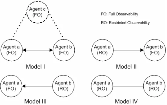
Definition 3: An agent i has full observability if it can observe the global system state.

→Zi. It is assumed that only these two types of observability exist within an n-agent

DEC-ROMDP.

Definition 4: Given an n-agent DEC-ROMDP and a current joint policy δ= (δ1, δ2…δn),

the steady state probabilities can be defined as ( , ,..., ) | | 2 1 δ δ δ δ ₌ S x x x

x , where xδk

represents the long run probability that the system state is k and |S| is the cardinality of set

S.

Definition 5: Given an n-agent DEC-ROMDP and a current joint policy δ= (δ1, δ2…δn),

the relative values can be defined as vδ =(v₁δ,...,v_|δ_S|) where

S s v p r v g S s s s s s

s = + ⋅ ∀ ∈

+

∑

Refer to Howard (1960) for more detail on relative values.

Definition 6: Given an n-agent DEC-ROMDP and a current joint policy δ= (δ1, δ2…δn), the associated expected reward is defined as Φ(δ), which is also called the gain, denoted

as_gδ _.

Definition 7: Given an n-agent DEC-ROMDP and a current joint policy δ= (δ1, δ2…δn), the following operation is called an individual policy update by agent i.

• If agent i has full observability, find a new individual policy 'δ_i which satisfies

) ( max arg ) ( ' ' ' )) ( ),..., ( , ), ( ),..., ( ( ' , )) ( ),..., ( , ), ( ),..., (

(1 1 1

∑

∈ ∀ ∈ + ⋅ = − + − + S s s s s a s s s s s s a s s s A a

i s r p v

n i i i n i i i i i δ δ δ δ δ δ δ δ δ δ S s∈ ∀ .

• If agent i has restricted observability, find a new individual policy 'δi which satisfies

] ) ( [ max arg ) ( ' ) ( ' ' )) ( ),..., ( , ), ( ),..., ( ( ' , )) ( ),..., ( , ), ( ),..., ( ( , ) ( 1 1 1 1 1 1

∑

∑

i G s z

S

s s S

s s s a s s s s s s a s s s s A a z s G S s

i s x r p v

δ δ δ δ δ δ δ δ δ δ δ i i Z z ∈ ∀ .

Note the above update keeps individual policies unchanged for every agent except agent

Lemma 1: Given an n-agent DEC-ROMDP and a current joint policy δ= (δ1, δ2…δn), after a policy update by agent i, the joint policy becomesδ'=(δ₁,...,δ_i−1,δ_i ,'δ_i+1,...,δ_n).

• If agent i has full observability, it is guaranteed thatΦ(δ')≥Φ(δ).

• If agent i has restricted observability, it is not guaranteed thatΦ(δ')≥Φ(δ).

Proof: If agent i has full observability, the agent faces a COMDP problem by fixing the

other agents' policies. A policy update can be treated as a policy improvement step in Howard's (1960) procedure which guaranteesΦ(δ')≥Φ(δ). If agent i has restricted

observability, the agent faces a ROMDP problem by fixing other agents’ policies. A policy update can be treated as a policy improvement step in the heuristic algorithm for solving a ROMDP problem. According to Chapter 2, this does not

guaranteeΦ(δ')≥Φ(δ). However, if this happens, the agent has found a local optimum

for that ROMDP problem. (Q.E.D)

Definition 8: A policy update by agent i from δ= (δ1, δ2…δn), to

1 1 1

δ' (= δ ,...,δi− ,δi′,δi+,...,δn) is called a policy improvement ifΦ(δ')≥Φ(δ).

Definition 9: A joint policy δ= (δ1, δ2…δn) is called local optimal policy if no policy improvement exists from any agent while fixing the other agents’ individual policies. The gain associated with the local optimal policy is called local optimal gain.

Definition 10: A joint policy δ= (δ1, δ2…δn) is called a jointmyopic policy if a

s A a

r s

∈

=

δ( ) argmax ,∀s∈S. That is, a joint myopic policy chooses an action which

maximizes the immediate expected reward for each state.

3.3 DEC-ROMDP Algorithm

This chapter introduces an evolutionary coordination algorithm that updates one agent’s policy while keeping other agents’ policies unchanged. There exist two

δ←Initialize joint policy, the gain δ

g ← Φ(δ), and fail←0

whilefail < ndo fori = 1 to n

policy update from δ= (δ1, δ2…δn) to δ'=(δ1,...,δ_i−1,δ_i ,'δ_i+1,...,δ_n)

if this policy update is a policy improvementthen

δ _(δ')

g ← Φ , δ←δ', fail ←0

else

fail←fail+1

iffail = nthen

break return gδ and δ.

Algorithm II

δ← Initialize joint policy, the gain _gδ _{← Φ(δ), and fail← 0}

whilefail < ndo fori = 1 to n

improved ← 0

while true do

policy update from δ= (δ1, δ2…δn) to

) ,..., ,'

, ,..., (

'= δ₁ δ_{i 1} δ_i δ_{i 1} δ_n

δ _{− +}

if this policy update is a policy improvementthen

δ _(δ')

g ← Φ , δ←δ', improved ← 1

else

break

ifimproved = 1 then

fail ← 0

else

fail ←fail+1

iffail = nthen break return gδ and δ.

Theorem1: The above algorithms monotonically increase expect reward, and eventually

will terminate at a local optimal policy after a finite number of iterations.

Proof: Both of the algorithms perform a policy update on an agent. If this policy update

does not improve the current policy, the next agent is selected to perform the policy update. Hence, the policy is monotonically increasing. As the expected reward is