The Simulation and Approximation of the First Passage Time of the Ornstein--Uhlenbeck Process of Neuron

Abstract

JIANG, LIQIU. The Simulation and Approximation of the First Passage Time of the Ornstein–Uhlenbeck Process of Neuron. (Under the direction of Charles Eugene Smith.)

THE SIMULATION AND APPROXIMATION OF THE FIRST PASSAGE TIME OF THE ORNSTEIN-UHLENBECK PROCESS OF NEURON

By

Liqiu Jiang

A thesis submitted to the Graduate Faculty of North Carolina State University

in partial fulfillment of the requirements for the Degree of

Master of Science

BIOMATHEMATICS GRADUATE PROGRAM DEPARTMENT OF STATISTICS

Raleigh

2002

APPROVED BY

___________________________ Dr. Charles E. Smith

BIOGRAPHY

Liqiu Jiang was born September 26, 1974 in Jilin Province, People Repub-lic of China. She received her elementary and secondary education in Jilin province, P. R. China and graduated from Meheikou Fifth High School in 1992.

ACKNOWLEDGEMENT

Contents

List of Tables . . . .viii

List of Figures . . . ix

1 Introduction 1 2 Literature Review 5 2.1 The Biological Background . . . 5

2.2 The Physical Basis for the LIF Model . . . 7

2.3 The Models . . . 12

2.3.1 The Ornstein–Uhlenbeck Model . . . 12

2.3.2 Stein’s model . . . 16

2.4 Approximation of the First Passage Time . . . 18

3 Methods 25

3.1 Simulation . . . 25

3.1.1 Testing for the Independence of Random Numbers . . 26

3.1.2 Euler Method . . . 28

3.1.3 Parameter . . . 31

3.1.4 Goodness–of–fit–test . . . 32

3.2 Approximation . . . 35

3.2.1 Approximation of Moments of the FPT . . . 35

3.2.2 Confidence Limits for the mean and variance of Log-normal Distribution . . . 42

3.2.3 Approximation Error . . . 44

3.2.4 Approximation of Probability Density Function of the FPT . . . 45

3.3 Comparison of Two Probability Density Functions . . . 47

4 Results 55 4.1 Simulation . . . 55

4.2 Approximation . . . 72

5 Discussion 94

6 Conclusions 98

Bibliography 100

List of Tables

List of Figures

2.1 The equivalent circuit of cell membrane with three ions . . . 8 2.2 The equivalent circuit of cell membrane . . . 9 2.3 The trajectory of the membrane voltage with uniform input current 14 3.1 Serial correlation coefficient at lag k with n 1000 . . . 52 3.2 The joint histogram of the random numberXi andXi+1 withn 1000 53

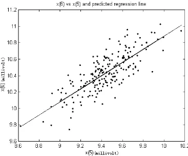
3.3 Scatter plot of the random number: Xi+1 against Xi with n 1000 . . . 54

Chapter 1

Introduction

The first passage time is the theoretical counterpart of the interspike inter-vals. This follows the generally accepted hypothesis that the information transferred within the nervous system is usually encoded by the timing of spikes (action potential). Therefore, the reciprocal relationship between the frequency on one hand and the interspike interval on the other leads to the study of the distribution of the first passage time. When the distribution is too difficult to obtain, the analysis is usually restricted to its moments, primarily the mean and variance.

the membrane depolarizaion is described as a deterministic leaky integrator. Interspike intervals are identified as periods between a reset of the depolariza-tion after firing (an acdepolariza-tion potential or a spike) and the consecutive crossing of a fixed firing threshold. This leaky integrate–and–fire model is one of the most common on both application of artificial neural network and descrip-tion of biological systems and has been studied in [37], [24], [36], [23],[9] and [30].

The OU process has the following properties: the voltage difference be-tween the membrane potential and resting potential at the trigger zone of the neuron is described by a one–dimensional stochastic processX ={X(t) : t ≥0} given by the stochastic differential equation

dX(t) = µ(X(t), t)dt+σ(X(t), t)dW(t), X(0) =x₀ (1.1)

consecutive neuronal firings (spikes). The reference level for the membrane potential is usually taken to be the resting potential. Some studies examined the effect of random initial values in a leaky integrator with deterministic trajectory. They found that different distributions for the initial value lead to commonly observed interspike interval distributions [18], [21], and [20]. This is why initial voltage (the reset value following a spike) is often as-sumed to be equal to the resting potential, x₀ = 0, i. e., there is no initial afterhyperpolarization. The OU process is appropriate for neurons with a high number of synaptic inputs where each of them has only a slight effect on the cell excitability [27].

Chapter 2

Literature Review

2.1

The Biological Background

potential, occurs when the potential exceeds a critical threshold and ionic concentrations achieve supercritical values.

The biophysical properties of the membrane have important effects on the action potential generation and conduction. For example, the passive resistive electrical properties of the post synaptic cell affect the time course of the postsynaptic cell potentials generated in it by other cells. The passive electrical properties of the postsynaptic cell also determine how efficiently synaptic potentials are propagated within a cell from their sites of origin to the trigger zone. These features of neuronal functioning contribute to synap-tic integration, the process by which a nerve cell adds up all incoming signals and determines whether or not it will generate an action potential. Once an action potential is generated, the speed with which it is conducted from the trigger zone to the axon terminal also depends on the passive electrical properties of axon.

the lipid bilayer, and the ionic concentration gradient (N a+_{, Cl}−_{, K}+_).

Al-though they are biological, the three electrical properties of the membrane are functionally indistinguishable from those of a man-made electronic circuit.

2.2

The Physical Basis for the LIF Model

Figure 2.1 is a complete equivalent circuit of the passive electrical properties of the membrane, with membrane capacitance included. Figure 2.2 is the simplified electrical equivalent circuit that can be used to examine the effects of membrane capacitance on the response of a neuron to injected current. The cell membrane is represented by a capacitor (C) in parallel with a re-sistor (R), which represents the RN a, RCl, and RK element in Figure 2.1.

The membrane batteries representing the electromotive forces generated by ion diffusion determine the resting or equilibrium voltage when there are no applied currents. It can be ignored because batteries affect only the absolute value of membrane voltage, not voltage rate of change.

Im =Ii+Ic (2.1)

Figure 2.1. The equivalent circuit of cell membrane with three ions.

Ii:Ionic (or resistive) membrane current represents the actual movement of

ions through the ion (conductance) channels of the membrane. Ic :

proportional to the charge (Q) stored on the capacitor:

V = Q

C (2.2)

Figure 2.2. The equivalent circuit of cell membrane. So, for a change in voltage

∆Vm = ∆

Q

This ∆Q is brought about by the flow of capacitive current (Ic). Also,

cur-rent is defined as the net movement of positive charge per unit time. The value of capacitive current is equal to the rate at which charge stored on the capacitor changes:

Ic =

dQ

dt (2.4)

Obviously, we can obtain ∆Qby integrating Ic over time.

∆Q=

t₂ t₁

Icdt (2.5)

By substituting to Equation (2.3), we obtain ∆Vm ≈

_t2

t₁ IcCdt.

The time course of Vm is slowed by the membrane capacitance. When

the Vm is changed by the current injected into the cell, ∆Vm lags behind the

into the capacitor to change the charge on its plates. However, as the pulse continues and ∆Q increases, more and more current must flow through the resistance, because at any instant the voltage drops across the membrane resistor

∆Vm =ImR (2.6)

must be equal to the voltage across the capacitor

∆Vm =

∆Q

C . (2.7)

As a larger fraction of the membrane current flows through the resistor, less is available for charging the capacitor; thus the rate of change ofVm decreases

with time. When ∆Vm reaches its plateau value, all of the membrane current

is flowing through the resistor and

Vm =ImR (2.8)

capacitor discharges and drives current through resistor. So, we can describe the potential change by the following equation (a usual exponential charging relationship [39]):

∆Vm(t) =ImR(1−e−

t

τ_{), (2.9)}

Where τ equals RC, the product of the resistance and capacitance of mem-brane. The parameter τ is called the membrane time constant.

2.3

The Models

2.3.1

The Ornstein–Uhlenbeck Model

The most common diffusion model is the OU process, which is one substan-tial step closer to reality than other models, since the spontaneous changes of the membrane potential are included in the model [25].

an action potential is considered to have infinitesimally small duration, the period of each action potential is just the time between interspike intervals. At the spike onset, the membrane capacitor discharges instantaneously, and the membrane potential is reset to the resting potential. This firing process repeats itself as long as the input current is on. The output of a neuron is the sequence of firing. This model is a classic leaky integrate–and–fire model. If we let µbe the input current, then µ= _CI, when the input is on. So, we can rewrite Equation 2.9 as:

dx dt =−

x

τ +µ (2.10)

where x=v. Then,

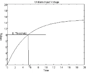
Figure 2.3. The trajectory of the membrane voltage with uniform input current. The rest curve approaches asymptote which is the product of µ and

τ, 15. The straight horizontal line is the threshold, S = 10. As we defined,

t∗ is the time at which mean of membrane voltage passes the threshold.

threshold. So,

t∗ =−τ log(1− S

µτ) (2.12)

Figure 2.3 plotted by Matlab shows that the mean trajectory of voltage, where x₀ is 0, µ, uniform input current, is 3 mvolt/msec, τ, membrane constant, is 5 msec, S, threshold, is 10 mvolt. We obtain t∗ is 5.4931 msec. Those values are reasonable parameters for neuron cell, in the spinal cord for example.

Equation 2.10 is easy to interpret. The more abstract OU process can be meaningfully derived. Equation 2.10 can arrive at the stochastic leaky integrator just by adding white noise

dx= (−x

is the moment of the previous firing of an action potential. In the case of suprathreshold stimulation, the model assumes that at each moment of firing, which is mimicked by reaching a firing threshold S, the membrane potential is reset to its initial value, X₀ = 0 [43]. Solving the stochastic differential equation, we can obtain

E[x(t)] =µτ(1−e−τt_{) (2.14)}

V ar[x(t)] = σ

2_τ

2 (1−e −2t

τ_{) (2.15)}

The OU process has been studied in [2], [31], [32], [33], and [8]. Some sophisticated numerical methods for the first passage time problem have been developed. But, no analytical solution for the OU process is known.

2.3.2

Stein’s model

of the model and its modifications and generalizations have been one of the most common approaches to the theoretical study of neuronal activity, such as in [20], [35], [27], [16], [18], [42], and [46]. The inputs of Stein’s model are divided into excitatory and inhibitory ones and follow Poisson processes. The heuristical stochastic differential equation is

dx dt =−

x τ +aE

dNE

dt −aI dNI

dt , (2.16)

where τ is membrane constant, NE and NI are independent simple

Pois-son processes with mean rates λE and λI. The trajectories of NE and NI

have discontinuities of +1 each time an excitatory or inhibitory input arrives. Hence the derivatives dNE/dtand dNI/dt, which appear in Equation (2.16),

consist of a collection of delta functions concentrated at the random arrival times of the synaptic inputs. When an excitatory input arrives, xwill jump by +aE mvolt, whereas when an inhibitory input arrivesx will jump by−aI

mvolt. The mean and variance of the depolarization in Stein’s model are [43]

E[x(t)] = τ(aEλE −aIλI)(1−e−

t

τ_{), (2.17)}

V ar[x(t)] = 1 2τ(a

2

EλE+a2IλI)(1−e−

2t

τ_{). (2.18)}

2.4

Approximation of the First Passage Time

To study the properties of the models themselves, approximation methods for model are very useful sometimes. Charles E. Smith summarized the approximation methods for the first passage time in [37] and [36]. We are interested in the case with deterministic crossing. The term ”deterministic crossing” will be used when the mean voltage crosses a threshold, S. Our description is a simple generalization of the method for Stein’s model. In this article, we also call it Stein’s method. Letr(t) =S−E[x(t)] be the recovery process following a spike, where S is the threshold. Besides requiring that the mean voltage crosses S, i. e. deterministic crossings, we require that

1. The membrane voltage distribution does not change its shape drasti-cally near t∗.

corre-lation time of x(t) around t∗.

3. r(t) is invertible and sufficiently smooth.

Let h be the inverse function of r(t), that is , h[r(t)] = t. Then, a pdf of first passage time, g(S, t|x₀), is approximately f(x)|dh(x)/dx| evaluated at t∗, where f(x) is the marginal distribution of S −x(t∗). This is the usual Jacobian transformation of random variables, i. e., we are treating the mem-brane voltage process like a singular random process. For example, if f(x) is Gaussian or normal and r(t) is a decaying exponential,g(S, t|x₀) is approxi-mately lognormal.

In many cases, we may only be interested in the first few moments of the FPT. The function h is now expanded in a Taylor’s series about r(t∗). The approximations for the mean and variance are given next with y=r(t), and µn is the nth central moment of the random variableS−x(t∗) [29]:

E(t)≈t∗+h(y)µ2 2! +h

_(y)µ3

3!+,· · · (2.19)

V ar(t)≈(h)2µ₂+hhµ₃−(hµ2 2! +h

µ3

3!)

where prime denotes differentiation with respect to membrane voltage. The expressions of the first four derivatives of h[r(t)] are in the section 3.2.1 on page 35. Stein’s original approximation method was the first term of Equa-tions (2.19) and (2.20). Then,

E(t) =t∗, (2.21)

and

V ar(t) =

dx dt

₂

V ar[x(t)]. (2.22)

been studied in [2], [32], [33], [17], [8], and [22].

Stein’s method is expected to work for the OU process under some condi-tions. For example, we expect it to perform best when the excitatory post– synaptic potential (EPSP) and inhibitory post–synaptic potential (IPSP) amplitudes are small and input frequencies are large. The diffusion approxi-mation therefore has infinitesimal mean

aEλE −aIλI−x≈µ−x, aE, aI >0, (2.23)

and infinitesimal variance

a2_EλE +a2IλI ≈σ2. (2.24)

2.5

Distribution Comparison Method

The analysis of neural spike trains has a long history [43]. There are two main approaches for such analysis. The first is to formulate a stochastic model for the neuron’s activity and inputs, derive the distribution of the FPT, and use it to fit the model to data. The stochastic process is often modelled as a random walk such as Stein’s model or an diffusion model such as the OU process. Another important approach in such a study is to fit standard families of densities to the FPT, such as the lognormal or gamma, using maximum likelihood or some ad hoc technique. So, another trial is that we want to compare the approximated FPT distribution derived by us-ing Stein’s method with the lognormal distribution fitted for the simulated FPT of the OU process.

In many cases, there is not enough information to assume that the candi-date families contain the true distribution that is generating the data. This is certainly the case for the problem at hand. So, we leave the true distribu-tion for the FPT histograms unspecified; using the simuladistribu-tion data, we then seek to identify the distribution which is closer to the true and unknown distribution.

[6], Nishii(1988) [28] and White(1982) [45]. We now describe the approach in general , and then specialize it to the case of the lognormal versus the approximated distribution. To assess the closeness of two densities f and p on the real line, we use Kullback–Leibler information criterion (or divergence)

I[p:f] =

_∞

0

p(x)log

p(x) f(x)

dx. (2.25)

It is known that I[p : f] ≥ 0, with equality only when p = f [45]. For example, if p(x) = µe−µx and f(x) = λe−λx for x > 0 and zero otherwise, then I[p:f] =λ/µ−1−log(λ/µ), which is 0.09 when the ratio of the means of these exponential densities is λ/µ= 1.5. Next, ifp and f are normal den-sities with means µand ν, respectively, and both variances equal to 1, then I[p:f] = (µ−ν)2_{/2, which is 0.125 when |µ−ν|= 0.5.}

Kullback–Leibler information criterion is not a metric. But, it does have an advantage over metrics for the problem of comparing two approximations f₁ and f₂ to an unknown densityp. Specifically,

I[p:f₁]−I[p:f₂] =

_∞

0

p(x)log

f₂(x) f₁(x)

= Ep

logf2(Y) f₁(Y)

(2.26)

where Ep refers to expectation with respect to the density p, which

gener-ates the random variable Y. In practice, given independent and identically distributed data (Y₁, . . . , Yn) from p, an estimate of Ep is

1 n

n

1

log

f₂(Yi)

f₁(Yi)

. (2.27)

Chapter 3

Methods

3.1

Simulation

constant threshold S.

3.1.1

Testing for the Independence of Random

Num-bers

In the case of two random variables (X, Y), a random sample of sizenconsists of the n pairs (Xi, Yi), i = 1,2, . . . , n. The sample correlation coefficient is

often defined as

R=

_n

i=1(Xi−X¯)(Yi−Y¯)

(n_i=1(Xi−X¯)2)(

n

i=1(Yi−Y¯)2)

, (3.1)

where

¯ X = 1

n n i=1 Xi and ¯ Y = 1

n

n

i=1

Yi

are the sample means forXandY [44]. Value of R close to zero indicates that X and Y are uncorrelated, which sometimes implies they are independent, for example, they are from a normal distribution. In the present situation we are concerned with a sequence of random variables X₁, X₂, . . . , Xn.

can regard the first member of each pair as one variable and the second mem-ber as another variable. The correlation coefficient of the first and second variables is called the serial correlation coefficient at lag 1:

R₁ =

n−1

i=1(Xi−X¯∗)(Xi+1−X¯∗∗)

(n_i=1−1(Xi−X¯∗)2)(

n−1

i=1(Xi+1−X¯∗∗)2)

(3.2)

where

¯

X_∗ = 1 n−1

n−1

i=1

Xi

is the mean of the first n−1 variables and

¯

X_∗∗ = 1 n−1

n−1

i=1

Xi+1

is the mean of the last n−1 variables.

It is possible, however, that consecutive variables are independent. But, for example, the pairs (X₁, X₃),(X₂, X₄),· · ·,(Xn₋2, Xn), are not

indepen-dent. Thus, we also compute a correlation coefficient for Xi and Xi+2. In

Rk =

n−k

i=1(Xi−X¯)(Xi+k−X¯)

_n

i=1(Xi−X¯)2

. (3.3)

Furthermore, under the assumption of independence, Rk is, when n is large,

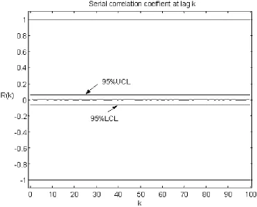
providingk n, approximately normal with mean zero and variance 1/n. It is useful to plot Rk versus k to obtain a serial correlogram. Figure 3.1 shows

that all values of Rk of the random numbers which our program generated

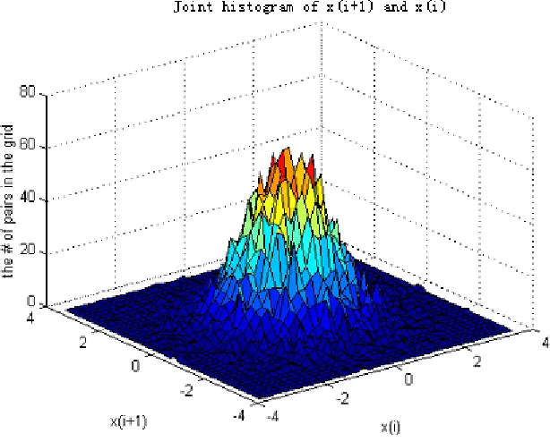
by using Matlab lie in the interval of [−1.96/√n,1.96/√n], where n is 1000 and k is in the interval [1, 100]. Another way is to use the joint histogram. Figure 3.2 is the joint histogram of Xi andXi+1. The joint histogram of two

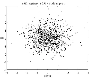
independent normal random variable has a symmetry ”mountain” shape, just as shown in Figure 3.2. Figure 3.3 is the scatter plot of random number Xi

against Xi+1. Those figures give the evidence for that Xi and Xi+1 are

inde-pendent.

3.1.2

Euler Method

be obtained by a mesh of points ti such that t0 < t1 < · · · < tn = T, and

ti+1−ti = ∆t. Equation (1.1) on t0 ≤t ≤ T with the initial value xt₀ =x0

can then be rewritten as

x(ti+1) =x(ti) + (−

x(ti)

τ +µ)(ti+1−ti) +σ(x(ti), ti)(W(ti+1)−W(ti)). (3.4)

This is an Euler approximation which is a discrete time stochastic process x(t) satisfying the iterative Equation (3.4). The procedure for solving Equa-tion (1.1) is to compute x(ti+1) from the knowledge of x(ti) realizing that

the increments of the standard Wiener process

∆Wi =Wi+1−Wi (3.5)

appearing in Equation (3.4) are mutually independent, normally distributed r.v.’s with mean zero and variance (ti+1−ti) independent of X(ti) [15]. We

use Matlab to generate random numbers of the increments of the Wiener process with mean µ= 0 and variance σ2 _{= ∆t.}

n, those for which xn is not sufficiently close to x0. The error in the linear

approximation formula

Y(xn+1)≈yn+h·f(xn, yn) = yn+1 (3.6)

is the amount by which the tangent line at (xn, yn) departs from the solution

curve through (xn, yn). This error, introduced at each step in the process,

is called the local error in Euler’s method. Besides local error, yn itself

will introduce roundoff errors 1000 times as often as one withh= 0.1 [5]. In our study, we choose h= 0.1 to do the simulation.

The average time for the sample path ofx(t) to approach to its asymptote is about 20 msec (see Figure 2.3). Because the ∆T we will use is 0.1 msec, to make sure that all the sample path ofx(t) to approach to its asymptote in our program, we let tn be 100 msec which is much greater than the average

time for the sample path of x(t) to approach to its asymptote. So, n in our program is 1000.

3.1.3

Parameter

For any quantitative discussion about the models and their mutual com-parison, at least the approximation about their parameters is necessary. The most appropriate would be to estimate these parameters from the data recorded intracellularly according to the model construction. So, we use rea-sonable parameters of a neuron in the spinal cord for µ, τ and S. For the Wiener process parameter σ2 _{we can only speculate. From the diffusion}

Wiener parameters in the OU process comes immediately from the experi-mental data in [11], where direct estimation from FPT has been performed. In their paper the estimated values of the parameterσ goes up to 15. We also referred to parameter values in [3], [41], [42], and [24] to pick the σ values which are shown in Table 3.1.

Table 3.1. Parameter values used in this study.

Parameter Value Units

τ 5 msec

µ 3 mvolt/msec

σ varies (0.5, 2, 4) mvolt/msec

S varies (6–14) mvolt

3.1.4

Goodness–of–fit–test

tests, which test the null hypothesis that the distribution is in some specified form. We use the D test developed by D’Agostino in 1971. It is one of most powerful tests available for detecting departures from a hypothesized normal or lognormal density function when n is between 50 and 1000. D’Agostino shows that his test compares favorably with other tests in its ability to reject H₀, when H₀ is actually false.

Suppose we wish to test the null hypothesis that the underlying distribu-tion is normal. Then the D test is conducted as follows:

1. Draw a random samplex₁, x₂, . . . , xnof sizen ≥50 from the population

of interest. n is 400 in this study.

2. Order the n data from smallest to largest to obtain the sample order statistics x_[1] ≤x_[2] ≤. . .≤x_[n].

3. Compute the statistic

D=

_n

i=1[i− 12(n+ 1)]x[i]

n2_s , (3.7)

s= 1 n n i=1

(xi−x¯)2

₁/2

. (3.8)

4. TransformD to the statistic Y by computing

Y = D−0.28209479

0.02998598/√n (3.9)

Ifnis large and the data are drawn from a normal distribution, then the expected value of Y is zero. For nonnormal distributions Y will tend to be either less than or greater than zero, depending on the particular distribution.

5. Reject at the α significance level the null hypothesis that the n data were drawn from a normal distribution ifY is less than theα/2 quantile or greater than the 1 −α/2 quantile of the distribution of Y. For n = 400, andα= 0.05, the upper and lower limit are 1.633 and -2.270, respectively [7].

3.2

Approximation

First, we go to the details of approximating the first two moments of the FPT (mean and variance).

3.2.1

Approximation of Moments of the FPT

• The First Four Derivatives of h[r(t)]

h[r(t)] = t, i. e., h(x) is the inverse function of r(t). Recall that the first derivative of an inverse function can be expressed as the reciprocal of the derivative of the original function [40]. Then, we take derivative of the first order derivative to get second order derivative, and so on.

h[r(t)] = [r(t)]−1 (3.10)

h[r(t)] = −[r(t)]−3r(t) (3.11) h[r(t)] = 3[r(t)]−5[r(t)]2−r(t)[r(t)]−4 (3.12) h[r(t)] = −15[r(t)]−7[r(t)]3+ 10[r(t)]−6r(t)r(t)

−r(t)[r(t)]−5 (3.13)

The First Four Derivatives ofh[r(t)] evaluated att∗ at which the mean of x(t) passes the threshold S. We can get the following by taking derivatives to r(t) and plugging in t∗ =−τ log(1− _µτs ) to r(t).

r(t) =−µe−τt _{, r(t}∗_{) =}−_(µ− s

τ) (3.14)

r(t) = µ τe

−t

τ _{, r(t}∗_{) =} 1

τ(µ− s

τ) (3.15)

r(t) = −µ τ2e

−t

τ _{, r(t}∗_{) =}− 1

τ2(µ−

s

τ) (3.16)

r(t) = µ τ3e

−t

τ _{, r(t}∗_{) =} 1

τ3(µ−

s

τ) (3.17)

After substituting to the derivatives of h[r(t)], we can obtain

h(t∗) = −(µ− s τ)

−1 _(3.18)

h(t∗) = 1 τ(µ−

s τ)

−2 _(3.19)

h(t∗) = − 2 τ2(µ−

s τ)

−3 _(3.20)

h(t∗) = 6 τ3(µ−

s τ)

−4 _(3.21)

• The nth central moment (µn) of the normal distribution N(µ, σ2)

n is even,n = 2k, the following is the formula for it.

E[(x−µ)2k] = (2k)!σ

2k

k!2k (3.22)

So, µ₃ =µ₅ = 0 andµ₄ = 3σ4,µ₆ = 15σ6. • The Taylor’s series of h[r(t)]

E(t) =t∗+hµ2 2! +h

µ3

3! +h µ4

4! +. . .+h

nµn

n! (3.23)

where un is nth central moment of S−x(t∗).

• The Taylor’s series of the variance of h[r(t)]

As we know

V ar(t) = V ar[h(r(t))] =E(h(r(t))2)−[E(h(r(t)))]2. (3.24)

letting g(t) = [h(r(t))]2_{, we can writeE([h(r(t}∗_))]2_{) as}

E([h(r(t∗))]2) = g(t∗) +g(t∗)µ2 2! +g

_(t∗₎µ3

3! +g

_(t∗₎µ4

4! +. . .+g

n

The first four derivatives of g(t) are

g(t) = 2h(t)h(t) = 2hh (3.26)

g(t) = 2[h(t)]2+ 2h(t)h(t) = 2h2+ 2hh (3.27) g(t) = 6h(t)h(t) + 2h(t)h(t) = 6hh+ 2hh (3.28)

g(t) = 6[h(t)]2+ 8h(t)h(t) + 2h(t)h(t)

= 6h2+ 8hh+ 2hh (3.29)

If we use the original Stein’s method to do the approximation, the mean and variance of FPT are

E(t) =−τ log(1− s

µτ) (3.30)

and

V ar(t) = 1 2

τ S(2µτ −S) (µτ −S)2_µ2 σ

2_{. (3.31)}

E(t) =t∗+hµ2

2! =−τ log(1− s µτ) +

1 4

S(2µτ −S) (µτ −S)2_µ2σ

2 _(3.32)

For the variance of FPT we need to calculate theE[h2_(r(t∗_{))] and [E(h(r(t}∗_)))]2_,

E[h2(r(t∗))] =h2+ (2h2+ 2hh)µ2

2! (3.33)

[E(h(r(t∗)))]2 = (h+hµ2 2!)

2_{, (3.34)}

where h is h[r(t∗)]. So, the variance of FPT is

V ar(t) = E([h(r(t∗))]2)−[E(h(t∗))]2 = h2µ₂− h

2_µ2 2

4 . (3.35)

Then we plug in h(r(t∗)) and obtain

V ar(t) = τ

2

(µτ −S)2σ 2

x−

τ2

4(µτ −s)4σ 4

where σ2

x isV ar[x(t∗)],

σ2(x) = σ

2_s

µ −

σ2s2 2µ2_τ =

s(2µτ −s) 2µ2_τ σ

2_{. (3.37)}

So, the variance of FPT can be written as

V ar(t) = S(2µτ −S)

2

2µ2_(µτ −_S)σ

2₋ S2(2µτ −S)4

4µ4_(µτ −_S)4σ

4 _(3.38)

If we use first four terms to do the approximation, then the mean of FPT is

E(t) = t∗+hµ2 2! +h

µ3

3! +h µ4

4! = −τ log(1− s

µτ) + 1 4

S(2µτ −S) (µτ −S)2_µ2σ

2 ₊ 3

16

S2(2µτ −S)2 τ(µτ −S)4_µ4σ

4

(3.39)

For the variance of FPT, the calculation steps are as following,

E[h2(r(t∗))] =h2+(2h2+2hh)µ2 2!+(6h

_h+2hh)µ3

3!+(6h

2_+8hh+2hh)µ4

[E(h(r(t∗)))]2 = (h+hµ2 2! +h

µ3

3! +h µ4

4!)

2 _(3.41)

So,

V ar(t) = E([h(r(t∗))]2)−[E(h(t∗))]2

= h2µ₂+hhµ3 + (6h2+ 8hh)µ4 24−

h2µ2₂ 22 +

h2µ2₃ 62 +

h2µ2₄ 242

+2hh µ3µ4 6×24 + 2h

_hµ2µ3

2×6+ 2h

_h µ2µ4

2×24 (3.42)

V ar(t) = τ

2

(µτ −s)2σ 2

x+

5τ2

2(µτ −s)4σ 4

x−

3τ2

4(µτ −s)6σ 6

x−

9τ2

16(µτ −s)8σ 8

x

(3.43)

V ar(t) = s(2µτ −s)τ 2(µτ −s)2_µ2σ

2₊5s2(2µτ −s)2

8(µτ −s)4_µ4 σ

4₋ 3s3(2µτ −s)3

32(µτ −s)6_τ2_µ6σ

6₋ 9s4(2µτ −s)4

256(µτ −s)8_τ2_µ8σ 8

3.2.2

Confidence Limits for the mean and variance of

Lognormal Distribution

There are several methods for calculating confidence limits. They are given in [7]. We use a simple method to estimate the mean µ and variance σ2 _of

the two–parameter lognormal distribution. SupposeX is random variable of lognormal distribution, let Y =log(X), so,

¯ y= 1

n

n

i=1

yi (3.45)

s2_y = 1 n−1

n

i=1

(yi−y¯)2. (3.46)

Then, we replace µy and σ2y by ¯y and s2y in the formulas for the true and

unknown µ and σ2_{. We get}

ˆ µ=e

¯

y+s2₂y

and

ˆ

σ2 = ˆµ2[es2y −_{1] (3.48)}

There are also several methods for calculating confidence limits for mean of lognormal distribution. Land’s method is considered as the best one. Land showed that the upper one-sided 100(1−α)% and the lower one-sided 100α% confidence limits for µare obtained by calculating

U L₁₋α =e

¯

y+0.5s2y+syH√n1−−1α

(3.49)

and

LLα =e

¯

y+0.5s2y+syHα√n−1

, (3.50)

respectively, where ¯yands2

y are calculated using Equations (3.45) and (3.46),

respectively. The quantities H₁₋α and Hα are obtained from the tables

pro-vided by Land in [7]. In our study, we use α= 0.05.

in a 100 time loop and get a sample of the variance. Then, we take the 97.5 percentile of the sample data as the upper confidence limit and 2.5 percentile of the sample data as the lower confidence limit. We repeat the procedure 10 times and obtain 10 confidence limits. We take the mean of the 10 percentiles as confidence limits of the variance.

We use the relationship between the approximation values of the mean and variance of FPT and the confidence interval of the simulatied mean and variance to tell if the approximation values are close enough to the simulation results. We conclude the approximation can work for those parameters if the approximation values fall in the confidence interval of the simulation data.

3.2.3

Approximation Error

If all the approximation values fall in the confidence interval no matter how many terms we used to approximate the mean and variance of FPT, we use the error of the approximation to tell which approximation is closer to the simulation data. It is defined as [42]:

E = Approximation−Simulation

=

Approximation

Simulation −1 100%. (3.51)

We use the mean and standard deviation of 100 E values for all the approx-imation value to estimate which approxapprox-imation method is better.

3.2.4

Approximation of Probability Density Function

of the FPT

The marginal distribution of x(t) is normal distribution with mean E(x(t)), which isµτ(1−e−τt_{), and varianceσ}2_τ(1−_e−2τt_{)/2. Then, the marginal}

dis-tribution forx(t∗) is N(−τ log(1−_µτs ), s(2µτ−s)

2µ2τ σ2). Obviously, E(x(t∗)) =S.

So, the marginal distribution for y=S−x(t∗) is N(0,s(2₂µτ_µ2−_τs)σ2).

fY(y(t∗)) =

1

2πs(2µτ−s) 2µ2τ σ2

e

−s(2µτ(y−)2s)

sµ2τ σ2 _(3.52)

The pdf of FPT g(s, t|x₀) is

g(s, t|x₀) =fYt∗(y)/

dh(y) dy

where

y=r(t) = S−E(x(t)) = µτ(1−e−τt_{). (3.54)}

and h(y) = h(r(t)) = −µe−tτ_{. So, the pdf of FPT approximated by using}

Stein’s method (Jacobian transform) is

g(s, t|x₀) = µe −t

τe−

(µτ(1−e−τt₎₋S)2 σ2τ₍₁₋₍₁₋S

µτ)2)

πσ2_τ(1−₍₁− S µτ)2)

, (3.55)

where t∈(0,∞).

The lognormal pdf estimated from simulation data is

fT(t) =

1 tσlog(t)

√ 2πe

−(log(₂t)_σ2−µlog(t))2

log(t) _(3.56)

where t ∈ (0,∞), µlog(t) is the mean of log(t) and σ2log(t) is the variance of

3.3

Comparison of Two Probability Density

Functions

We use Stein’s method to approximate the probability density function of the FPT. We estimate the lognormal density function by using the maxi-mum likelihood estimator [4]. Then, we can see which one is better for the simulation data by Kullback–Leibler information criteria.

First, we describe the general comparison of two probability density func-tions. We define

F ={f(y|α) :α∈A} (3.57)

and

G={f(y|β) :β ∈B} (3.58)

the member of F that minimizesI[p:f(·|α)], over α∈A, and defineβ_∗ ∈ B

similarly. Thus,

IF =IF[p:a_∗]=

_∞

0

p(y)log

p(y) f(y|a∗)

dy (3.59)

characterizes the proximity ofF top, andI_G=I_G[p:β_∗] (defined similarly) characterized the proximity of G to p. Thus, the difference

IG−IF =

_∞

0

p(y)log

f(y|α_∗) g(y|β_∗)

dy (3.60)

allows for a comparison of F and G, using estimates ofα_∗ and β_∗, which we describe next.

Given a random sample Y = (y₁, . . . , yn) generated from p(y), let the

quasi–log–likelihood function of α under F be

Ln(α|Y) = n

i=1

log[f(yi|α)] (3.61)

and a quasi–maximum likelihood estimator (QMLE) ˆαn be a value which

A natural estimate ofIG−IF is

Tn =

1 n n i=1 log

f(yi|αˆn)

g(yi|βˆn)

, (3.62)

which is asymptotically normal:

√

n[Tn−(IG−IF)]→N(0, σ2), (3.63)

where the variance σ2 _=E

p[log[f(Y|α∗)/g(Y|β∗)]]2 is estimated by

ˆ σ2 ₌ 1

n

n

i=1

logf(yi|αˆn) g(yi|βˆn)

₂

. (3.64)

The regularity conditions that guarantee the existence of the quasi–true pa-rameters α_∗ and β_∗, the consistency of ˆσ2

n are described in the papers by [6],

[45], and [28]. These conditions are satisfied for the comparison below. We omit the details of that verification.

H₁ : IG = IF. We then compute the statistic

√

nTn and its estimated

standard deviation ˆσn. Given a confidence coefficient α, we construct the

approximate confidence interval for (IG−IF),

In,α =

Tn+cα

ˆ σn

√

n, Tn−cα ˆ σn √ n (3.65)

wherecα is the upper 100(1−α/2) percent point of the standard normal

dis-tribution (if α= 0.05, cα = 1.96). If 0 ∈In,α, then we cannot reject the null

hypothesis that the two distributions are equally close to the true distribu-tion; otherwise we reject the null hypothesis. Furthermore, if In,α ⊆(0,∞),

we conclude that F is closer to the true model; if In,α ⊆ (0,−∞), we

con-clude that G is closer to the true distribution. We now turn to the specifics for lognormal distribution. The QMLEs ˆαn = ( ˆα1n,αˆ2n) for lognormal are

obtained from Equations (3.66) and (3.67).

ˆ α₁n =

1 n

n

1

log(yi) (3.66)

ˆ α₂n=

1 n

n

1

Figure 3.1. Serial correlation coefficient at lag k with n is 1000. k is be-tween [1,100]. The central irregular line is Rk. The two straight lines are

upper confidence limit and lower confidence limit, respectively, as labelled.

The random numbers are generated from a standard normal distribution with

Figure 3.2. The joint histogram of random numbers Xi and Xi+1, where

Figure 3.3. Scatter plot of the random numbers: Xi+1 against Xi with n

Chapter 4

Results

4.1

Simulation

1. The correlation time of the OU process .

process (at least 5 msec) is greater than the standard deviations of the corresponding FPT. The largest standard deviation of the FPT is 2.5 mesc, when the threshold is 14 mvolt. Most are less than 1 msec. This could also be obtained from the Stein’s approximation method, in section 2.4 on page 18. Thus, the OU process has a long correlation time compared to the resultant standard deviation of FPT.

From the sample paths in Figures 4.5, 4.6, and 4.7, we can see the sample paths are always on one side of the expected mean membrane voltage for a while before they cross their expected mean. The corre-lation of the membrane voltage is apparent over short time ranges.

2. The marginal distribution of membrane voltage is the normal distributed.

D’Agostino’s test results for the marginal distribution of x(t).

time 5 10 15 20 25 30 35

Y 0.5172 0.3746 0.8196 0.6536 1.5296 1.8049 0.9387

The sample size of the x(t) is 400. All the Y values are in the interval (-2.270,1.633). So, we do not reject the null hypothesis and conclude

that all the variables x(t) follow normal distribution.

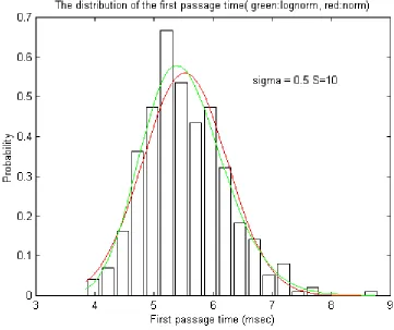
3. The lognormal distribution is very close to the distribution of FPT.

Table 4.2. D’Agostino’s test results for distribution of the FPT.

Threshold, S σ

mvolt 0.5 2 4

7 -1.6975 -0.2848 0.8183 10 -1.4606 0.0411 1.5692 13 -1.0100 0.3651 0.8468

The sample size of the FPT is 400. All the Y values are in the interval

(-2.270, 1.633). So, we do not reject the null hypothesis and conclude

Figure 4.5. A sample path of the membrane voltage with the Wiener pro-cess parameter 0.25 (the irregular curve). The central smooth curve is the expected mean of membrane voltage and the two smooth curves beside it are

the upper and lower 95% confidence limit, respectively. The horizontal line

Figure 4.6. A Sample path of the membrane voltage with the Wiener process parameter 4 (the irregular curve). The central smooth curve is the expected mean of membrane voltage and the two smooth curves beside it are the upper

and lower 95% confidence limit, respectively. The horizontal line represents

Figure 4.7. A Sample path of the membrane voltage with the Wiener pro-cess parameter 16 (the irregular curve). The central smooth curve is the expected mean of membrane voltage and the two smooth curves beside it are

the upper and the lower 95% confidence limit, respectively. The horizontal

Figure 4.8. The histogram and pdfs of membrane voltage of the OU pro-cess at 5 mesc. The total area of histogram bars is 1. The blue curve is pdf of the simulated membrane voltage, and the green curve is the pdf of

ex-pected membrane voltage at 5 mesc. The sample size of the random variable

Figure 4.9. The histogram and pdfs of membrane voltage of the OU pro-cess at 15 mesc. The total area of histogram bars is 1. The blue curve is pdf of the simulated membrane voltage, and the green curve is the pdf of expected

membrane voltage at 5 mesc. The sample size of the membrane voltage is

Figure 4.10. The histogram and pdfs of the membrane voltage of the OU process at 25 mesc. The total area of histogram bars is 1. The blue curve is pdf of the simulated membrane voltage, and the green curve is the pdf of

ex-pected membrane voltage at 5 mesc. The sample size of the random variable

Figure 4.11. The histogram and the pdfs of FPT of the OU process with the Wiener process parameter 0.25 and the threshold 10 mvolt. The green curve is fitted by lognormal density function and the red curve is fitted by

Figure 4.12. The histogram and the pdfs of FPT of the OU process with the Wiener process parameter 4 and the threshold 10 mvolt. The green curve is fitted by lognormal density function and the red curve is fitted by

Figure 4.13: The histogram and the pdfs of FPT of the OU process with the Wiener process parameter 16 and the threshold 10 mvolt. The green curve is fitted by lognormal density function and the red curve is fitted by

4.2

Approximation

1. For the small Wiener process parameter, Stein’s approxima-tion values of the mean and variance of FPT are close to the simulated results.

When σ is 0.5, Figures 4.14 and 4.15 show that the mean and variance approximated using the Stein’s method are very close to the simulated results. This is true except when the threshold is 14 mvolt. This tells us the approximation using Stein’s method works well for a small Wiener parameter. Forσ = 2, Figures 4.15 and 4.16 show that the ap-proximated results deviate from the simulated results a lot, when the thresholds are greater than 9mvolt. Whenσis 4, Figures 4.18 and 4.19 show that the approximation results deviate from the simulated results very much, even if the threshold is very small. All the approximation results are out of the confidence interval (CI) of the simulated results. This result suggests that the Stein’s method should not be used near the large Wiener parameter range in OU process.

results are like Stein’s method for the small Wiener parame-ter. But, this does not work well for a large Wiener process parameter.

When σ is 0.5, after adding the second term of the Taylor’s series to Stein’s method, approximation results are all very close to the simula-tion results. Figures 4.20 and 4.21 show this, except when threshold is greater than 12 mvolt.

When σ is 2, Figures 4.22 and 4.23 show that the approximation re-sults still deviate from the simulation rere-sults a lot, for large thresholds. They also show that by using more terms, the deviations even occur for the small thresholds. Figures 4.24 and 4.25 tell us that for a large Wiener process parameter, σ is 2 or 4, the approximation does not work. All approximation results deviate from the simulation results a lot, particularly for large thresholds, such as 14 mvolt.

3. The approximation errors of two terms of the Taylor’s series are less than those of one term, when σ is 0.5.

Figure 4.14. Stein’s approximation for the mean of FPT by using the first term of the Taylor’s series , where the Wiener process parameter is 0.25.

The central curve is the mean of membrane voltage from simulation and the

other two curves beside it are the upper and lower 95% confidence limit for

the mean FPT, respectively. ”*” represents the approximation values by the

Figure 4.15. Stein’s Approximation for the standard deviation of FPT by using the first term of the Taylor’s series, where The Wiener process pa-rameter is 0.25. The central curve is the mean of membrane voltage from simulation and the other two curves beside it are the upper and lower 95%

confidence limit respectively. ”*” represents the approximated values by the

Figure 4.16. Stein’s approximation for the mean of FPT by using the first term of the Taylor’s series, where the Wiener process parameter is 4. The central curve is the mean of membrane voltage from simulation and the other

two curves beside it are the upper and lower 95% confidence limit for the

mean FPT, respectively. ”*” represents the approximated values by the first

Figure 4.17. Stein’s Approximation for the standard deviation of FPT by using the first term of the Taylor’s series, where the Wiener process parame-ter is 4. The central curve is the mean of membrane voltage from simulation and the other two curves beside it are the upper and lower 95% confidence

limit respectively. ”*” represents the approximated values by the first term of

Figure 4.18. Stein’s approximation for the mean of FPT by using first term of the Taylor’s series, where the Wiener process parameter is 16. The central curve is the mean of membrane voltage from simulation and the other two

curves beside it are the upper and lower 95% confidence limit for the mean

FPT, respectively. ”*” represents the approximated values by the first term

Figure 4.19. Stein’s Approximation for the standard deviation of FPT by using the first term of the Taylor’s series, where the Wiener process parame-ter is 16. The central curve is the mean of membrane voltage from simulation and the other two curves beside it are the upper and lower 95% confidence

limit respectively. ”*” represents the approximated value by the first term of

Figure 4.20. The Approximation for the mean of FPT by using two terms of the Taylor’s series and four terms, where the Wiener process parameter is 0.25. The central curve is the mean of membrane voltage from simulation and the other two curves beside it are the upper and lower 95% confidence

limit, respectively. ”*” represents the approximated values by the first term

of the Taylor’s series; ”+” represents the approximated values by two terms;

Figure 4.21. The Approximation for the standard deviation of FPT by using two terms of the Taylor’s series and four terms, where the Wiener process parameter is 0.25. The central curve is the standard deviation of membrane voltage from simulation and the other two curves beside it are the upper and

lower 95% confidence limit, respectively. ”*” represents the approximated

values by the first term of the Taylor’s series; ”+” represents the

approxi-mated values by two terms; ”◦” represents the approximated values by four

Figure 4.22. The Approximation for the mean of FPT by using two terms of the Taylor’s series and four terms, where the Wiener process parameter is 4. The central curve is the mean of membrane voltage from simulation and the other two curves beside it are the upper and lower 95% confidence limit,

respectively. ”*” represents the approximated values by the first term of the

Taylor’s series; ”+” represents the approximated values by two terms; ”◦”

Figure 4.23. The Approximation for the standard deviation of FPT by using two terms of the Taylor’s series and four terms, where the Wiener process pa-rameter is 4. The central curve is the standard deviation of membrane voltage from simulation and the other two curves beside it are the upper and lower

95% confidence limit, respectively. ”*” represents the approximated values by

the first term of the Taylor’s series; ”+” represents the approximated values

Figure 4.24. The Approximation for the mean of FPT by using two terms of the Taylor’s series and four terms, where the Wiener process parameter is 16. The central curve is the mean of membrane voltage from simulation and the other two curves beside it are the upper and lower 95% confidence limit,

respectively. ”*” represents the approximated values by the first term of the

Taylor’s series; ”+” represents the approximated values by two terms; ”◦”

Figure 4.25. The Approximation for the standard deviation of FPT by using two terms of the Taylor’s series and four terms, where the Wiener process parameter is 16. The central curve is the standard deviation of membrane voltage from simulation and the other two curves beside it are the upper and

lower 95% confidence limit, respectively. * represents the approximation value

by first term of the Taylor’s series; + represents the approximation value by

Table 4.3. The approximation errors of the mean of FPT by the different terms of the Taylor’s series.

S(threshold) one term two terms four terms

mvolt errormean stderror errormean stderror errormean stderror

6 -0.0528 0.0063 -0.0482 0.0063 -0.0482 0.0063 7 -0.0418 0.0063 -0.0364 0.0063 -0.0364 0.0063 8 -0.0335 0.0054 -0.0271 0.0055 -0.0270 0.0055 9 -0.0265 0.0055 -0.0187 0.0055 -0.0185 0.0055 10 -0.0202 0.0063 -0.0103 0.0063 -0.0100 0.0063 11 -0.0129 0.0080 0.0006 0.0081 -0.0014 0.0081 12 -0.0048 0.0074 0.0158 0.0076 0.0179 0.0076

errormean represents the approximation errors of the mean of FPT. stderror

represents the standard deviation of the approximation errors. The sample

Table 4.4. The approximation errors of the standard deviation of FPT by the different terms of the Taylor’s series.

S(threshold) one term two terms four terms

mvolt errorstd stderror errorstd stderror errorstd stderror

6 -0.0003 0.0338 -0.0010 0.0338 0.0058 0.0340 7 0.0057 0.0370 0.0048 0.0370 0.0144 0.0373 8 0.0009 0.0386 -0.0003 0.0386 0.0133 0.0391 9 0.0137 0.0338 0.0118 0.0388 0.0319 0.0395 10 0.0129 0.0390 0.0101 0.0389 0.0405 0.0401 11 0.0287 0.0403 0.0240 0.0401 0.0738 0.0420 12 0.0582 0.0457 0.0493 0.0453 0.1412 0.0493

errorstd represents the approximation errors of the standard deviation of

FPT. stderror represents the standard deviation of the approximation errors.

4.3

Comparison of Two Probability Density

Functions

Figure 4.29. 95% confidence interval of the difference of Kullback–Leibler information criteria. The two irregular curves are the 95% upper and lower limit for the difference of Kullback–Leibler information criteria of the

Chapter 5

Discussion