EPQ Model with Time Dependent IHC and
Weibull Distributed Deterioration under
Shortages
Ankit Bhojak
1, U. B. Gothi
2Assistant Professor, Dept. of Statistics, GLS Institute of Commerce, GLS University, Ahmedabad, Gujarat, India.1
Associate Professor, Head, Dept. of Statistics, St. Xavier’s College (Autonomous), Ahmedabad, Gujarat, India.2
ABSTRACT: In this paper, we have developed an inventory model to determine the economic production quantity for deteriorating items under time dependent demand. Inventory holding cost is taken as a linear function depending upon time. A combination of two parameter and three parameter Weibull distribution is considered for the deterioration of units over a period of time. For practical applicability, shortages are allowed to occur. Besides that we have assumed that demand is a linear and also quadratic function of time in different time intervals. A numerical example is given for the developed model with its sensitivity analysis.
KEYWORDS: EPQ model, Deterioration, Backlogging, Weibull distributions I. INTRODUCTION
The classic Economic Production Quantity (EPQ) model is a mathematical model which determines the lot size in production processthat minimizes the total inventory holding cost and set up cost. In classic EPQ model demand for an item is assumed to be continuous with constant rate. Further production of items is also assumed to be continuous with constant rate. Many researchers suggested different EPQ models by changing some of the assumptions of classic EPQ model by assuming the time varying production rate, deterioration rate, shortages and quantity discount.
An inventory model for deteriorating items with time-dependent demand and time-varying holding cost under partial backlogging developed by Mishra V.K., Singh L.S. & Kumar R. [18]. Ankit Bhojak and U. B. Gothi [1] prepared an EOQ model with time dependent demand and Weibull distributed deterioration. Wu J. W. and Lee W. C. [25] presented an EOQ inventory model for items with Weibull distributed deterioration, shortages and time varying demand. Ghosh S. K. and Chaudhari K. S. [11] have given an order-level inventory model for a deteriorating item with Weibull distribution deterioration, time-quadratic demand and shortages.
Cheng, Huei-Hsin Chang and Singa Wang Chiu [8] presented economic production quantity model with backordering, rework and machine failure taking place in stock piling time. Jinn-Tsair Teng, Liang-Yuh Ouyang and Chun-Tao Chang [13] formed deterministic economic production quantity model with time-varying demand and cost. R. Shamsi, A. Haji, S. Shadrokh and F. Nourbakhsh [19] formulated an economic production quantity in reworkable production systems with inspection errors, scraps and backlogging. U. B. Gothi and Devyani A. Chatterji [24] have developed an EPQ model for imperfect quality items under constant demand rate and varying inventory holding cost.
Samanta G. P. and Roy Ajanta [20] presented a production inventory model with deteriorating items and shortages. Madhu Jain, G.C. Sharma and Shalini Rathore [16] developed an economic production quantity models with shortage, price and stock-dependent demand for deteriorating items. Sugapriya C. and Jeyaraman K. [22] have given an EPQ model for non-instantaneous deteriorating item in which holding cost varies with time. Sarkar S. and Chakrabarti T. [21] presented an EPQ model having Weibull distribution deterioration with exponential demand and production with shortages under permissible delay in payments. Kirtan Parmar and U. B. Gothi [14] formulated an EPQ model of deteriorating items using three parameter Weibull distribution with constant production rate and time varying holding cost.
Sunil V. Kawale and Pravin B. Bansode [23] developed an inventory model for time varying holding cost and Weibull distribution for deterioration with fully backlogged shortages Devyani Chatterji and U. B. Gothi [7] formulated an inventory model by considering combination of two parameters and three parameters Weibull distribution in different time intervals and partially backlogged shortages. In this paper we have developed an EPQ model having demand as a mixer of linear and quadratic function of time in different time intervals with fully backlogged shortages.
II. ASSUMPTIONS
The model is developed under the following assumptions 1. Replenishment rate is infinite.
2. Lead-time is zero.
3. A single item is considered over the prescribed period of time.
4. No repair or replacement of the deteriorated items takes place during a given cycle. 5. Finite time horizon period is considered.
6. Holding cost is a linear function of time given by Ch = h + r t (h, r > 0).
7. The deterioration rate is a two parameter Weibull distribution during the time interval [0 , µ] and during the time interval [µ , t1] it is three parameter Weibull distributed deterioration rate.
8. Shortages are allowed and all unsatisfied demands are fully backlogged
9. Total inventory cost is a real and continuous function which is convex to the origin. III. NOTATIONS
The following notations are used to develop the mathematical model 1. Q (t) : Inventory level of the product at time t ( ≥ 0). 2. R (t) : Demand rate varying over time.
3. θ (t) : Deterioration rate.
4. A : Ordering cost per order during the cycle period. 5. Ch : Inventory holding cost per unit per unit time.
6. Cd : Deterioration cost per unit per unit time.
7.
Cs : Shortage cost per unit per unit time.8.
Cp : Production cost per unit.9. S1 : Inventory level at t = µ.
10. S2 : The maximum inventory level during shortage period.
IV.MATHEMATICAL FORMULATION AND SOLUTION
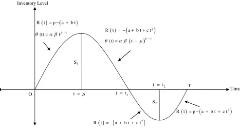
In the beginning inventory is zero. At time t = 0, the production starts and supply also starts simultaneously. The production stops at t = µ where the maximum inventory level S1 is reached. In the interval [0, µ] the inventory is built
up at a rate p – (a + b t) along with the deterioration rate. The stock level falls to zero level at time t = t1 due to demand
with rate – (a + b t + c t 2) along with the deterioration rate. Thereafter, shortages are allowed to occur during the time interval at a rate – (a + b t + c t 2). At time t = t2 shortage reaches to maximum level S2 and the backlog is fulfilled
at a rate of p – (a + b t + c t 2) in the time interval [t2, T]. The stock level becomes zero at time t = T. The same cycle is
repeated for the further time period T. The graphical presentation of inventory model is shown in Figure 1.
Figure 1 Graphical representation of inventory model
Differential Equations pertaining to the above situation as explained are given by
1
d Q t
t Q t p a + b t 0 t dt
... (1)
1
2
1
d Q t
t Q t a b t + c t t t dt
... (2)
2
1 2
d Q t
a b t + c t t t t
dt ... (3)
2
2
d Q t
p a b t + c t t t T
dt ... (4)
Using the boundary conditions
1
Q 0 Q t Q T 0, Q
S , Q t1
2 S2
1(t) = t
2
R t = a b t + c t
2
R t = p a b t c t
Time T
2
R t = a b t c t
1
(t) = t
R t = p a b t
Inventory Level
O t
t t1
2
t t
S1
the solutions of equations (1), (2), (3) and (4) are given by
b t2
p a
t 1 b t
2
Q t = p a t2 1 2 2
... (5)
2 3
1
1 2 3
1
y t c t
Q t S 1 t z t
2 3
z t y t c t
+ + +
1 2 2 3 3
... (6)
2 2
3 3
1 1 1
b c
Q t a t t t t t t
2 3
... (7)
b
2 2
c
3 3
Q t p a t T t T t T
2 3
... (8) where y 2 c + b and z a + b + c 2
Putting Q t
1 0 in equation (6), we get
2 3 1
1 1 1
1
1 2 3
1 1 1
y t c t z t
z t
2 3 1
1 S
1 t y t c t
2 2 3 3
... (9)
Putting Q t
2 S2 in equation (7), we get
2 2
3 3
2 2 1 2 1 2 1
b c
S a t t t t t t
2 3
... (10)
Putting Q t
2 S2 in equation (8), we have
2 2
3 3
2 2 2 2
b c
S p a T t T t T t
2 3
... (11)
From equation (10) and (11)
2 2
3 3
2 1 1 1
1 b c
t T a T t T t T t
p 2 3
... (12)
The total cost consists of the following costs (1) Operating Cost
OC = A ... (13)
(2) Production Cost
c 2
(3) Inventory Holding Cost
t1
0
IHC h + r t Q t dt h + r t Q t dt
22 3 3
3
3 4 4
1
1 1
p a
b b
h p a
2 6 1 2 2 2 3 p a
b b
r p a
3 8 1 3 2 2 4 t
+ h + r S t
1 2 3 4
1 1 1
2 3 4
1 1 1
z t y t c t
1 2 6 12
z t y t c t + + +
1 2 2 2 3 3 3
2 2 3 4 5
1 1 1 1 1
1
3 4
1 1 1
4 t t z t y t c t
+ r S
2 2 3 8 15
z t y t c t + +
1 3 2 2 4
53 3 5
... (15)
(4) Deterioration Cost
t1
1 1
d 0
DC C t Q t dt t Q t dt
1 2
1 1
d
+ 1 + 2 + 3
1 1 1
p a b S t
C
1 2 2
z t y t c t
+ 1 2 + 2 3 + 3
... (16)
(5) Shortage Cost
2 1 2 t T s t tSC C Q t dt Q t dt
2 3 2 2 3 3 4 4
s 1 1 1 2 1 2 1 2 1 2 1
2 3
2 2
2 2
3 3 4 4
2 2
b c a b c
C a t t t t t t t t t t t
2 3 2 6 12
p a b T c T
p a T T t T t
2 3 2
b c
T t T t 6 12 ... (17)
Hence, the average total cost per unit time is
1
TC A + IHC DC + SC + PC T
2
2 3 3
3
3 4 4
1 1
p a
b b
h p a
2 6 1 2 2 2 3
p a
b b
r p a
3 8 1 3 2 2 4
t + h + r S t
A + 1 T
1 2 3
1 1 1
4 2 3 4
1 1 1 1
2 1 1
z t y t
1 2 6
c t z t y t c t
+ + +
12 1 2 2 2 3 3 3 4
t + r S
2
2 3 4 5
1 1 1 1
3 4 5
1 1 1
t z t y t c t
2 3 8 15
z t y t c t
+ + +
1 3 2 2 4 3 3 5
+ 11 2
1 1 1
d
+ 2 + 3
1 1
s
p a b S t z t
1 2 2 + 1
C
y t c t
2 + 2 3 + 3
a C
2 3 2 2 3 3 4 4
1 1 1 2 1 2 1 2 1 2 1
2 3
2 2 3 3 4 4
2 2 2 2
p 2
b c a b c
t t t t t t t t t t t
2 3 2 6 12
p a
b T c T b c
p a T T t T t T t T t
2 3 2 6 12
+ C T t p
... (18) Our objective is to determine optimum values t1 and Tof t1 and T respectively so that TC is minimum. Note that t1
and Tare the solutions of the equations
1
TC TC 0 & 0 t T
... (19)
1 1
1 1
2
2 2 2
2 2
1 1
t t , T = T
2
2
1 t t , T = T
TC TC TC
0 t T
t T
TC 0 t ... (20)
V. NUMERICAL EXAMPLE
Let us consider the following example to illustrate the above developed model. We consider the following values of the parameters A = 200, α = 0.0001, β = 4, h = 6, r = 1.5, Cs= 3, Cd = 5, p =2500, Cp = 7, a = 2, b = 1.7, c = 0.1 & µ = 7
(with appropriate units of measurement). We obtain the optimal values t1 = 12.516462527627823 and
T= 54.750912148555784 units and optimal total cost TC = 22732.871686290677 units. VI.SENSITIVITY ANALYSIS
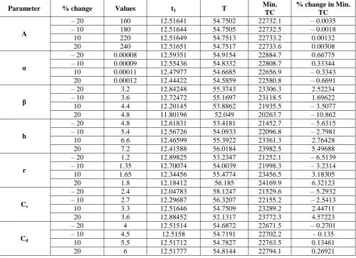
Sensitivity analysis helps in identifying the effect of optimal solution of the model by the changes in its parameter values. In this section, we study the sensitivity of total cost per time unit TCwith respect to the changes in the values of the parameters A, α, β, h, r, Cs, Cd, p, Cp, a, b, c and µ.
The sensitivity analysis is performed by considering 10% and 20% increase and decrease in each one of the above parameters keeping all other remaining parameter as fixed. The results are presented in Table – 1. The last column of table shows the % change in TC as compared to the original solution corresponding to the change in parameters values.
Parameter % change Values t1 T
Min. TC
% change in Min. TC
A
– 20 160 12.51641 54.7502 22732.1 – 0.0035 – 10 180 12.51644 54.7505 22732.5 – 0.0018 10 220 12.51649 54.7513 22733.2 0.00132 20 240 12.51651 54.7517 22733.6 0.00308
α
– 20 0.00008 12.59351 54.9154 22884.7 0.66775 – 10 0.00009 12.55436 54.8332 22808.7 0.33344 10 0.00011 12.47977 54.6685 22656.9 – 0.3343 20 0.00012 12.44422 54.5859 22580.8 – 0.6691
β
– 20 3.2 12.84248 55.3743 23306.3 2.52234 – 10 3.6 12.72472 55.1697 23118.5 1.69622 10 4.4 12.20145 53.8862 21935.5 – 3.5077 20 4.8 11.80196 52.049 20263.7 – 10.862
h
– 20 4.8 12.61831 53.4181 21452.7 – 5.6315 – 10 5.4 12.56726 54.0933 22096.8 – 2.7981 10 6.6 12.46599 55.3922 23361.3 2.76428 20 7.2 12.41588 56.0184 23982.5 5.49688
r
– 20 1.2 12.89825 53.2347 21252.1 – 6.5139 – 10 1.35 12.70074 54.0039 21998.3 – 3.2314 10 1.65 12.34456 55.4774 23456.5 3.18305 20 1.8 12.18412 56.185 24169.9 6.32123
Cs
– 20 2.4 12.04783 58.1247 21529.6 – 5.2932 – 10 2.7 12.29687 56.3207 22155.2 – 2.5413 10 3.3 12.51646 54.7509 23289.2 2.44711 20 3.6 12.88452 52.1317 23772.3 4.57223
Cd
– 20 4 12.51514 54.6872 22671.5 – 0.2701 – 10 4.5 12.5158 54.7191 22702.2 – 0.135
-30 -20 -10 0 10 20 30
-20-10 10 20 -20-10 10 20 -20-10 10 20 -20-10 10 20 -20-10 10 20 -20-10 10 20 -20-10 10 20
A β r Cd Cp b µ
%
c
h
a
n
g
e
in
M
in
.
T
C
% change in parameters p
– 20 2000 12.26263 51.8364 19292.8 – 15.133 – 10 2250 12.39725 53.3492 21039.2 – 7.4504 10 2750 12.62312 56.0588 24380.7 7.24853 20 3000 12.71935 57.2862 25988 14.3189
Cp
– 20 5.6 12.47311 54.6441 22083.1 – 2.8584 – 10 6.3 12.4949 54.6981 22408 – 1.4292 10 7.7 12.53781 54.8027 23057.6 1.42833 20 8.4 12.55893 54.8534 23382.4 2.85709
a
– 20 1.6 12.51857 54.7748 22714.1 – 0.0827 – 10 1.8 12.51752 54.7629 22723.5 – 0.0413 10 2.2 12.51541 54.739 22742.3 0.04135 20 2.4 12.51436 54.727 22751.6 0.08226
b
– 20 1.36 12.58267 55.5429 22289.5 – 1.9505 – 10 1.53 12.54932 55.1416 22513.2 – 0.9664 10 1.87 12.4841 54.3705 22948.7 0.94928 20 2.04 12.45222 54 23160.7 1.88185
c
– 20 0.08 12.68717 56.8871 21931.4 – 3.5257 – 10 0.09 12.59842 55.7588 22345.1 – 1.7059 10 0.11 12.44035 53.8423 23098.2 1.60692 20 0.12 12.36931 53.0169 23443.8 3.12719
µ
– 20 5.6 11.05549 47.4194 16331.8 – 28.158 – 10 6.3 11.79522 51.1599 19461.6 – 14.39
10 7.7 13.21889 58.1414 26047.2 14.5793 20 8.4 13.90073 61.2535 29266.9 28.7425
Table – 1 Sensitivity Analysis
-30 -20 -10 0 10 20 30
-20 -10 10 20 -20 -10 10 20 -20 -10 10 20 -20 -10 10 20 -20 -10 10 20 -20 -10 10 20
α h Cs p a c
%
c
h
a
n
g
e
in
M
in
.
T
C
% change in parameters
The effect of the percentage change in the values of parameters on the percentage change in minimum total cost is presented in the graphical presentation of sensitivity analysis of the model parameters.
VIII.CONCLUSION
From the above sensitivity analysis we may conclude that the average total cost per unit time TC is highly sensitive to changes in the values of the parameters µ and p moderately sensitive to changes in the value of the parameters β, h, r, Csand less sensitive to changes in the values of the parameters Cp, c, b, α, Cd, a and A.
REFERENCES
[1] Ankit Bhojak and Gothi, U. B., “An EOQ Model with Time Dependent Demand and Weibull Distributed Deterioration”, International Journal of Engineering Research & Technology,Vol. 4, Issue 09, pp.109-115, 2015.
[2] Baten Azizul and Kamil Anton Abdulbasah, “Analysis of inventory-production systems with Weibull distributed deterioration”,International Journal of physical Sciences Vol.4(11), pp.676-682, 2009.
[3] Chaman Singh and Singh, S.R., “An EPQ Model with Power form Stock Dependent Demand under Inflationary Environment using Genetic Algorithm”. International Journal of Computer Application (0975-8887) Vol.48-No.15, 2012.
[4] Chang, H. C., “A Note on the EPQ Model with Shortages and Variable Lead Time”. Information and Management Sciences Vol. 15, No.1, pp.61-67, 2004.
[5] Chung-Ho Chen, “ The Modified Economic Manufacturing Quantity Model for Product with Quality Loss Function”. Tamkang Journal of Science and Engineering, Vol. 12, No. 2, pp.109-112, 2009.
[6] Chun-Hsiung Lan, Yen-Chieh Yu, Robert H.-J. Lin, Cheng-Tan Tung, Chih-Pin Yen and Peter Shaohua Deng, “A Note on the Improved Algebric Method for the EPQ Model with Stochastic Lead Time”. Information and Management Sciences Vol. 18, No.1, pp.91-96, 2007. [7] Devyani Chatterji and Gothi U. B., “EOQ Model For Deteriorating Items Under Two And Three Parameter Weibull Distribution And Constant
IHC With Partially Backlogged Shortages”. International Journal of Science, Engineering and Technology Research (IJSETR), Vol. 4, Issue 10, October 2015, pp.3582-3594, 2015.
[8] Feng-Tsung Cheng, Huei-Hsin Chang and Singa Wang Chiu, “Economic production quantity model with backordering, rework and machine failure taking place in stock pilling time”. Information Science and applications, Vol. 7,Issue 4, 2010.
[9] Garima Garg, Bindu Vaish and Shalini Gupta, “An Economic Production Lot Size Model with Price Discounting for Non-Instantaneous Deteriorating Items with Ramp-Type Production and Demand Rates”. Int. J. Contemp. Math. Sciences, Vol. 7, No. 11, pp.531 – 554, 2012. [10] GedeAgus Widyadana and Hui Ming Wee, “An economic production quantity for deteriorating items with preventive maintenance policy and
random machine breakdown”. International journal of system, science,Vol.43, pp.1870-1882, 2012.
[12] Hui- Ming Wee, Wan-Tsu Wang and Po-Chung Yang, “A production quantity model for imperfect quality items with shortage and screening constraint”. International journal of Production research. Vol.51, No.6, pp.1869-1884, 2013.
[13] Jinn-Tsair Teng, Liang-Yuh Ouyang and Chun-Tao Chang, “Deterministic economic production quantity model with time-varyig demand and cost”. Applied Mathematical Modelling 29, pp.987–1003, 2005.
[14] Kirtan Parmar and Gothi, U. B., “An EPQ model of deteriorating items using three parameter Weibull distribution with constant production rate and time varying holding cost”. International Journal of Science, Engineering and Technology Research, Vol. 4, pp.409 – 416, 2015. [15] Leopoldo Eduardo CaHrdenas-Barron, “The economic production quantity (EPQ) with shortage derived algebraically”. Int. J. Production
Economics 70, pp. 289-292, 2001.
[16] Madhu Jain, G.C. Sharma and Shalini Rathore, “Economic production quantity models with Shortage, price and stock-dependent Demand for deteriorating items”. IJE Transactions Vol. 20, No 2, pp.159-166, 2007.
[17] Mehdi Alimohamadi, Seyed Mojtaba Sajadi, Seyed Akbar and NilipourTabatabaie, “A New EPQ Model with Considering Preventive Maintenance, Imperfect Product, Shortage and Work in Process Inventory”. Interdisciplinary journal of contemporary research in business Vol.3,No 8., 2011.
[18] Mishra, V. K., Singh, L. S. and Kumar, R., “An inventory model for deteriorating items with time-dependent demand and time-varying holding cost under partial backlogging”. Journal of Industrial Engineering International, 2013.
[19] Shamsi, R., Haji, A., Shadrokh, S., and Nourbakhsh, F., “Economic Production Quantity in Reworkable Production Systems with Inspection Errors, Scraps and Backlogging”. Journal of Industrial and Systems Engineering Vol. 3, No. 3, pp.170-188, 2009.
[20] Samanta, G.P. and Roy Ajanta, “A Production Inventory Model with Deteriorating Items and Shortages”. Yugoslav Journal of Operations Research 14, No 2, pp.219-230, 2004.
[21] Sarkar, S. and Chakrabarti, T., “An EPQ model having Weibull distribution deterioration with exponential demand and production with shortages underpermissible delay in payments”. Mathematical Theory and Modeling, Vol.3, No.1, pp.1-6, 2013.
[22] Sugapriya, C. and Jeyaraman, K., “An EPQ model for non-instantaneous deteriorating item in which holding cost varies with time”. Electronic Journal of Applied Statistical Analysis, pp.16-23, 2008.
[23] Sunil V. Kawale and Pravin B. Bansode, “An Inventory Model for Time Varying Holding Cost and Weibull Distribution for Deterioration with Fully Backlogged Shortages”. International Journal of Mathematics Trends and Technology, pp.201-206, 2013.
[24] Gothi, U. B. and Devyani A. Chatterji, “EPQ model for Imperfect Quality Items Under Constant Demand Rate and Varying IHC”. Sankhya Vignan NSV11, 7 – 19, 2015.