Temporal Variation in Groundwater and VOC Flux through a Sandy Streambed, Wilson, North Carolina.

(1)

ABSTRACT

CLAY, KEVIN REX. Temporal Variation in Groundwater and VOC Flux through a Sandy Streambed, Wilson, North Carolina. (Under the direction of Dr. David Genereux.)

Groundwater-surface water exchange can be a significant factor in the flushing of volatile organic compounds (VOCs) from contaminated aquifers, but is rarely quantified and is an understudied aspect of VOC transport. Coupling thermal modeling and repeated

groundwater sampling in a streambed, time series of water flux (vf), VOC concentration ([VOC]), and VOC flux (fvoc) were produced at two points, 13 m apart, in an urban stream called Hominy Swamp Creek, in Wilson NC from December 2016 to March 2017. The two locations were referred to as 78L (78m downstream of the Goldsboro Street bridge, on the left side of the stream) and 91R (91m downstream of the bridge on the right side of the stream). 3-4 day vf time series were also produced at seven sites in Hominy Swamp Creek from late July to early October 2016, prior to Hurricane Matthew.

Temperature measurements were made using vertically oriented arrays of temperature loggers (HOBO TidbiT v2) called thermal profilers. Each temperature time series was

filtered to isolate its 24-hour component, and time series from the sensors within a profiler were used to produce hourly-scale estimates of vf using VFLUX 2, a set of MATLAB routines for calculating vertical water flux from raw temperature data. Groundwater samples were collected using steel piezomanometers every 3-4 days, and analyzed using gas

chromatography – mass spectrometry to find the concentrations of benzene,

(2)

conductivity and hydraulic head gradient). At site 91R, groundwater flow was consistently from the aquifer to the stream. [VOC] was generally below 3 μg L-1_{. At sites 78L during} December 2016 – February 2017 and 91R during January 2017 – February 2017, cis-DCE had the greatest mean concentration of any VOC (0.891 μg L-1 and 0.213 μg L-1 at sites 78L-B and 91R, respectively), benzene had the lowest (0.031 μg L-1 and 0.016 μg L-1 at sites 78L-B and 91R, respectively). Most fvoc values were between ±0.5 mg m-2 d-1. At sites 78L over December 2016 – February 2017 and 91R over January 2017 – February 2017, cis-DCE had the highest flux (mean fvoc of 0.064 and 0.044 mg m-2 d-1 at 78L and 91R, respectively), and benzene the lowest (mean fvoc of 0.002 and 0.003 mg m-2 d-1 at 78L and 91R, respectively). Even though mean [VOC] at 78L was higher than at 91R, 91R had higher mean fvoc, which can be attributed to consistently upward groundwater flow through the streambed at 91R (there were many reversals of flow at 78L). Linear regressions between vf and fvoc were significant at site 78L-B (but not at 91R).

By using temperature measurements and modeling, making daily-scale estimates of fvoc was possible without the need for wells or estimates of hydraulic conductivity.

Concentration data alone would not have allowed for accurate conclusions about the relative mass transport of VOCs at sites 78L and 91R. This, along with the correlations between vf and fvoc at site 78L, demonstrates the importance of quantifying vf when assessing

(3)

(4)

(5)

Temporal Variation in Groundwater and VOC flux through a Sandy Streambed, Wilson, North Carolina.

by Kevin Rex Clay

A thesis submitted to the Graduate Faculty of North Carolina State University

in partial fulfillment of the requirements for the degree of

Master of Science

Marine, Earth, and Atmospheric Science

Raleigh, North Carolina

2017

APPROVED BY

_______________________________ _______________________________

Dr. Detlef Knappe Dr. Joshua Heitman

_______________________________ Dr. David Genereux

(6)

DEDICATION

(7)

BIOGRAPHY

(8)

ACKNOWLEDGMENTS

(9)

Table of Contents

List of Figures ... vi

List of Tables ... viii

1. Introduction ... 1

2. Background on VOCs ... 3

2.1. VOCs Focused on in This Study ... 3

2.2. Benzene ... 3

2.3. cis-DCE ... 4

2.4. Vinyl Chloride ... 5

3. Study Area ... 5

4. Methods ... 8

4.1. Overview ... 8

4.2 Temperature Profiler Design ... 9

4.3. VFLUX 2... 12

4.4. Calculation of Vertical Water Flux ... 13

4.5 Groundwater Sampling and Analysis ... 21

4.6 Measurement of Soil Thermal Diffusivity and Volumetric Heat Capacity ... 22

5. Results and Discussion ... 23

5.1 Temperature Time Series ... 23

5.2 Water Flux ... 25

5.3. VOC Concentration and Flux ... 41

6. Summary/Conclusions ... 60

References ... 64

APPENDIX A. Mathematical Background ... 69

APPENDIX B. Uncertainty in vf, [VOC], and fvoc ... 73

APPENDIX C. Datasets for vf, [VOC], and fvoc ... 79

(10)

List of Figures

Figure 3.1: Location of Wilson, NC. Black lines represent county boundaries (data from

http://data.nconemap.gov/)...6

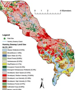
Figure 3.2: Land use in the Hominy Swamp Creek watershed. Data from the USGS national hydrography dataset (nhd.usgs.gov) and the 2011 national land cover database (NLCD; https://www.mrlc.gov/finddata.php)...7

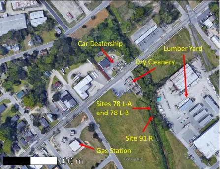
Figure 3.3: Google Earth image of Hominy Swamp Creek and adjacent properties (taken from Google Earth)...8

Figure 5.1: Raw and filtered temperature time series 8 cm deep in the streambed at site 78L-B. Time tick marks represent midnight at the start of the day shown in the tick mark label..24

Figure 5.2: Water flux (specific discharge) at site 54L. Water fluxes were calculated using the vflux_qar_opt addon (Irvine et al. 2017) in VFLUX 2. Positive values indicate upward flux...26

Figure 5.3: Water flux (specific discharge) at site 62LC. Water fluxes were calculated using the vflux_qar_opt addon (Irvine et al. 2017) in VFLUX 2. Positive values indicate upward flux...26

Figure 5.4: Water flux (specific discharge) at site 46RC in early August 2016. Water fluxes were calculated using the vflux_qar_opt addon (Irvine et al. 2017) in VFLUX 2. Positive values indicate upward flux...27

Figure 5.5: Water flux (specific discharge) at site 46LC in early August 2016. Water fluxes were calculated using the vflux_qar_opt addon (Irvine et al. 2017) in VFLUX 2. Positive values indicate upward flux...27

Figure 5.6: Water flux (specific discharge) at site 62LC in late September 2016. Water fluxes were calculated using the vflux_qar_opt addon (Irvine et al. 2017) in VFLUX 2. Positive values indicate upward flux...28

Figure 5.7: Water flux (specific discharge) at site 46LC in late September 2016. Water fluxes were calculated using the vflux_qar_opt addon (Irvine et al. 2017) in VFLUX 2. Positive values indicate upward flux...28

Figure 5.8: Water flux (specific discharge) at site 62RC. Water fluxes were calculated using the vflux_qar_opt addon (Irvine et al. 2017) in VFLUX 2. Positive values indicate upward flux...29

Figure 5.9: Water flux time series for both thermal profilers from Dec. 7, 2016 to Jan. 24, 2017. Water fluxes were calculated using the vflux_qar_opt addon (Irvine et al. 2017) in VFLUX 2. Tick marks represent 00:00 for each day...29

Figure 5.10: Water flux time series for both thermal profilers from Jan. 30, 2017 to Mar. 7, 2017. Water fluxes were calculated using the vflux_qar_opt addon (Irvine et al. 2017) in VFLUX 2. Tick marks represent 00:00 for each day...30

Figure 5.11: Water flux and daily precipitation at site 78L-B from 12/07/2016 to 3/10/2017. Tick marks represent 00:00 for each day...34

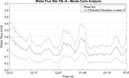
Figure 5.12: Monte Carlo analysis of vf at site 78L-A...38

Figure 5.13: Monte Carlo analysis of vf at site 78L-B...39

(11)

Figure 5.15: Comparison of β = 0 m (no thermal dispersion) versus β = 0.001 m for site 91R using unoptimized Ar fluxes. Tick marks represent 00:00:00 of each day...40 Figure 5.16: VOC concentrations at site 78L from 12/07/2016 – 02/20/2017. Tick marks represent 00:00:00 of each day...42 Figure 5.17: VOC concentration at site 78L from 1/31/2017 – 02/20/2017. Tick marks

represent 00:00:00 of each day...43 Figure 5.18: Water and VOC flux at site 78L-B. Tick marks represent 00:00:00 of each day...47 Figure 5.19: Water and VOC flux at site 78L-B from 01/31/2017 to 03/07/2017 (the period of data collection at site 91R). Tick marks represent 00:00:00 of each day...48 Figure 5.20: Water and VOC flux at site 91R. Tick marks represent 01:30:00 of each day...49 Figure 5.21: Linear regression of all water and benzene flux results at site 78L-B (except the 1/4/2017 outlier)...51 Figure 5.22: Linear regression of all water and vinyl chloride flux results at site 78L-B

(12)

List of Tables

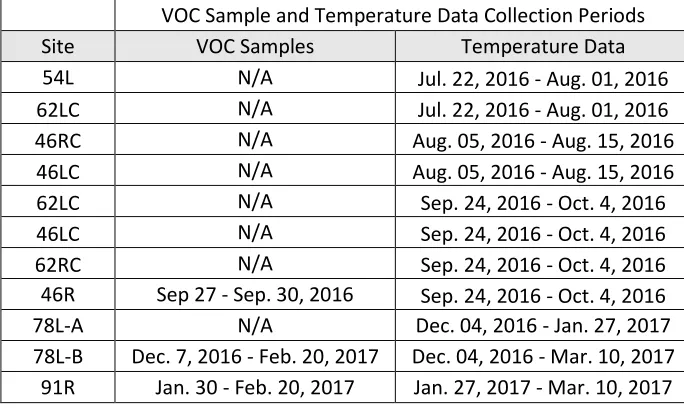
Table 1. Locations and periods of groundwater sample and temperature data

collection...11 Table 2. VFLUX parameter inputs and values used for this investigation...16 Table 3. Mean and range of vf (m/d) for different sites in HSC from late July 2016 to early March 2017. Streambed depth intervals in which the vf estimates were made (defined by the depths of the temperature sensors) are shown (3-10 cm, 10-17 cm, and 8-15 cm). Standard deviations are shown in parentheses. Positive vf corresponds to upward flow...31 Table 4. Mean calculated thermal diffusivity (m2/d) and sensor spacing (cm) for different sites in HSC from late July 2016 to early March 2017. Standard deviations are shown in parentheses. ... ...37 Table 5. Mean, standard deviation, and coefficient of variation for benzene (BZ), vinyl chloride (VC), and cis-DCE (cDCE) concentrations at both sites. The middle group columns (under Site 78L, 1/31-2/20) is included to compare statistics for sites 78L and 91R over that same time period. NA: not applicable, NM: not

(13)

1. Introduction

Volatile organic compounds (VOCs) are organic compounds conventionally distinguished by a vapor pressure above 0.13 kPa (Bloemen and Burn 1993). VOCs have seen widespread use in the US; VOC-bearing products have applications in a variety of settings including residential, commercial, and industrial (Zogorski et al. 2006; Carter et al. 2008; EPA 2009). Their widespread use, in addition to poor historical waste disposal practices, have resulted in VOCs being common soil and water contaminants (Carter et al. 2008).

In a nationwide study, 90 of 98 randomly selected aquifers were contaminated with VOCs in at least low concentrations (Zogorski et al. 2006), with VOCs more frequently detected in populated areas (Sequillace and Moran 2007). Many VOCs have a range of negative effects on human health, such as increased cancer risk, liver damage, and kidney problems (EPA 2009). VOCs may migrate with groundwater and enter public water supply wells and discharge into streams (Zogorski et al. 2006), leading to human and environmental exposure. Following discharge into streams, VOCs are diluted and volatilize into the air, which introduces inhalation as an exposure pathway.

VOC discharge to surface water is also a significant factor in the flushing and remediation of contaminated aquifers. Kim and Hemond (1998) found that an aquifer

contaminated by industrial activities in eastern MA discharged VOCs at a rate comparable to pump and treat systems employed at the site, making groundwater discharge an “alternative [aquifer] cleanup option in considering remedial strategies”. Chapman et al. (2007) found

(14)

μg/L near the source to as low as 20-50 μg/L about 350 m downgradient) was primarily due

to the TCE plume partly discharging into two streams and a pond as it intersected these surface water receptors along its flow path.

A multitude of techniques have been employed to quantify VOC discharge into surface water. Kim and Hemond (1998) used chemical tracers in conjunction with VOC concentration measurements. Calculation of chemical mass discharge across transects of wells (e.g Chapman et al. 2007; Guilbeault et al. 2005) is another approach. Some recent papers have coupled concentration measurements with in-stream head and K measurements (Ellis and Rivett 2007; Nickels 2016), and found that VOC discharge is sometimes

concentrated at “hot spots”.

These methods are useful, but have some limitations. Some of these techniques require knowledge of saturated hydraulic conductivity, which can vary over multiple orders of magnitude in the same stream (Genereux et al. 2008; Calver 2001). These methods also only provide a snapshot of VOC plume discharge, but flux conditions may change over time. The use of wells can become prohibitively expensive or limit locations these techniques can be employed.

The use of heat as a naturally occurring, omnipresent tracer does not require estimates of hydraulic conductivity and can produce continuous, hourly-scale estimates of groundwater flux through streambeds. The advantages of using heat as a tracer can overcome the

(15)

1. Use recently developed thermal modeling techniques to produce a high-frequency time series of water flux.

2. Couple water flux with repeated groundwater sampling to produce quantitative time series of vertical VOC flux through the streambed.

2. Background on VOCs

2.1. VOCs Focused on in This Study

VOCs have seen widespread use in the United States in a variety of settings for over a century. However, it was not until the 1970s that the environmental regulation along with the Environmental Protection Agency (EPA) took action to restrict the presence of VOCs in soil and water and minimize human exposure (Doherty 2000). The EPA began setting

enforceable Maximum Contaminant Levels (MCLs) in 1985, which restricts the

concentration of contaminants allowed in drinking water (Doherty 2000; EPA 2009). This investigation focuses on three VOCs – benzene (C6H6), vinyl chloride (C2H3Cl), and cis-dichloroethylene (cis-DCE; C2H2Cl2), all of which are commonly found at sites placed on the EPA National Priorities List (ASTDR 1996, 2007, 2014)

2.2. Benzene

Benzene’s widespread use gives it a multitude of ways to enter the environment.

(16)

water via discharge from industrial facilities, and gasoline and landfill leaks (ASTDR 2007; EPA 2009).

Benzene has a solubility of 1780 mg/L, and readily partitions into a gaseous phase with a Henry’s law constant of 5.5 x 10-3_{atm m}3_mol-1_{(Mackay and Lienonen 1975).} Benzene has a relatively low octanol-water partition coefficient (Kow) of 135 (Fetter 1993). The degradation of benzene can occur under aerobic conditions via oxidation as well as under anaerobic conditions (Vogel andGrbìc-Galìc 1986; Edwards and Grbìc-Galìc 1992). Benzene has a MCL of 0.005 mg/L (EPA 2009).

2.3. cis-DCE

Cis-DCE is used as a solvent, and in the production of perfumes and lacquers, among other things (ASTDR 1996). It is introduced into the environment through industrial

discharge, landfill leakage, and breakdown of chlorinated chemicals such as trichloroethylene (TCE) via reductive dechlorination. There are no consumer goods that are known to contain cis-DCE (ASTDR 1996; EPA 2009). Human exposure to cis-DCE can occur via inhalation or ingestion of contaminated tap water, which can cause liver complications (ASTDR 1996; EPA 2009). It is not currently known whether cis-DCE is a carcinogen (ASTDR 1996; EPA 2010).

(17)

anoxic conditions, converting TCE to cis-DCE, which degrades to vinyl chloride (Barrio-Lage et al. 1986; Vogel et al. 1987). cis-DCE has a MCL of 0.07 mg/L (EPA 2009).

2.4. Vinyl Chloride

Vinyl chloride is primarily used in the production of polyvinyl chloride (PVC), but has also been used as a coolant, propellant, and in some cosmetics (ASTDR 2014). Vinyl chloride is often introduced to the environment via leaching from PVC pipes and discharge from plastic factories or vinyl chloride manufacturing facilities (EPA 2009; ASTDR 2014). Like cis-DCE, vinyl chloride can be produced via the reductive dechlorination of chlorinated ethenes (Vogel et al. 1987). Vinyl chloride is carcinogenic via exposure from inhalation and ingestion (EPA 2000).

Vinyl chloride has a Henry’s law constant of 0.278 atm m3 mol-1 at 24.8°C and will quickly volatilize from surface water under most natural conditions (Gossett 1987). vinyl chloride has a Kow of 24 (Chu and Chan 2000), indicating it is somewhat mobile in soil. Under anaerobic conditions, vinyl chloride undergoes reductive dechlorination, converting it into ethylene (Vogel et al. 1987). Broholm et al. (2005) demonstrated the complete aerobic biodegradation of vinyl chloride in microcosms in 57 days. Vinyl chloride has a MCL of 0.002 mg/L (EPA 2009).

3. Study Area

Hominy Swamp Creek (HSC) is a stream located in the Neuse River Basin in eastern North Carolina. HSC originates in Wilson, NC (Fig. 3.1), and flows south through a

(18)

Bridge over HSC, adjacent to a site of groundwater contamination with dry cleaning chemicals; the site is known and monitored by the NC DEQ (e.g., Ranck and MacWilliams 2013, 2014). Prior to October 10, 2016, the date of heavy precipitation from Hurricane Matthew, the streambed was primarily sand, and the stream water depth at baseflow was generally in the range 10-40 cm. High flow following the hurricane eroded away about a meter of streambed in the area about 20-76 m downstream of Goldsboro Street, and the remaining streambed was much more clayey than before. The streambed also contains debris such as bricks, bottles, and tires.

Figure 3.1: Location of Wilson, NC. Black lines represent county boundaries (data from http://data.nconemap.gov/).

(19)

plumes affect this portion of HSC (Nickels, 2016). One plume is related to PCE and its degradation products, while the other contains benzene and other VOCs in lower

concentrations. The PCE related plume was discovered in 2004 and has been attributed to the operation of a nearby dry-cleaning facility that is only about 50 ft from HSC and has been in operation since 1959 (Ranck and MacWilliams 2013, 2014). PCE and its degradation

products have moved through the aquifer and into HSC. Recent reports on this contamination recommend annual groundwater and surface water monitoring rather than remediation

(Ranck and MacWilliams 2013, 2014). The other plume dominated by benzene seems to discharge into the opposite (east) side of HSC, though its exact point of origin is not currently known.

(20)

Figure 3.3: Google Earth image of Hominy Swamp Creek and adjacent properties (taken from Google Earth).

Nickels (2016) calculated and mapped VOC fluxes at the same location in mid-2015 and early 2016 using field permeameters and piezomanometers (Kennedy et al. 2007, 2009) in conjunction with VOC sampling. The VOCs with the highest fluxes through the HSC streambed were cis-DCE, vinyl chloride, and benzene, with the highest flux values being 195.1, 12.81, and 471.2 mg m-2_d-1_{, respectively, for these three VOCs.}

4. Methods

4.1. Overview

(21)

2012; Irvine et al. 2015b), temperature time series data were analyzed to produce hourly-scale estimates of vertical water flux through the streambed, i.e., the specific dicharge (vf), thermal diffusivity of the streambed (Ke), and sensor spacing (∆z) (the latter was generated as a check on the temperature data analysis, to see if the estimate from VFLUX 2 was close to the known sensor spacing). VOC concentration, [VOC], was measured in groundwater samples collected from a depth of 17-22 cm in the streambed, and VOC flux was quantified as fvoc = vf[VOC]. vf was obtained using an approach recently added to VFLUX 2 as

described in Irvine et al. (2017) and in section 4.4 of this thesis.

4.2 Temperature Profiler Design

Initially, four thermal profilers were built and used in preliminary measurements in HSC from July to early October 2016. These profilers were carried away downstream and lost due the streambed erosion from the high discharge following heavy rain on October 10, 2016 from Hurricane Matthew. Subsequently, two new profilers were built and deployed from December 3, 2016 to March 1, 2017.

The initial thermal profilers each contained three temperature loggers, inside a short (about 30.5 cm) section of 1.25 inch diameter PVC pipe. A PVC drivepoint was cemented onto one end of the pipe and a PVC cap sealed the other end. Installation of the thermal profilers began with inserting the PVC pipe in the streambed. After the pipe was inserted, the temperature loggers were inserted into the pipe, and a PVC cap was placed onto the open top end of the pipe.

(22)

positioned the sensors inside the PVC pipe at depths of 3, 10, and 17 cm below the top of the streambed. This enabled the temperature logger arrays to be removed for data downloading and re-inserted while keeping the sampling location constant (no movement of the PVC pipe). The HOBO loggers were chosen due to their inexpensive price ($133 per logger), acceptable accuracy (+/- 0.2 C) and resolution (0.02 C), and ability to operate under water. The deepest sensor pair, 10-17 cm depth, provided a reasonable tradeoff with respect to detection of the diurnal signal at depth, and sensitivity to changes in thermal diffusivity.The shallow pair of temperature sensors (3-10 cm depth) was to be used if the amplitude of the diurnal signal fell below 0.02°C and was used to assess changes in vertical water flux with depth, which has implications on whether the water flux has a significant lateral component (e.g., Cuthbert and McKay 2013). These thermal profilers collected brief temperature time series (5-11 days) at multiple locations from June to early October, 2016. These sites were along transects laid during previous work at HSC (Nickels 2016). The transects across HSC were spaced 8 m apart along the channel, from 30 to 78 m downstream of the Goldsboro Street bridge, and thermal profiler sites were along the eastern side of the creek to capture temperature time series where the streambed was consistently under water. Each

(23)

Table 1. Locations and periods of groundwater sample and temperature data collection.

VOC Sample and Temperature Data Collection Periods

Site VOC Samples Temperature Data

54L N/A Jul. 22, 2016 - Aug. 01, 2016

62LC N/A Jul. 22, 2016 - Aug. 01, 2016

46RC N/A Aug. 05, 2016 - Aug. 15, 2016

46LC N/A Aug. 05, 2016 - Aug. 15, 2016

62LC N/A Sep. 24, 2016 - Oct. 4, 2016

46LC N/A Sep. 24, 2016 - Oct. 4, 2016

62RC N/A Sep. 24, 2016 - Oct. 4, 2016

46R Sep 27 - Sep. 30, 2016 Sep. 24, 2016 - Oct. 4, 2016

78L-A N/A Dec. 04, 2016 - Jan. 27, 2017

78L-B Dec. 7, 2016 - Feb. 20, 2017 Dec. 04, 2016 - Mar. 10, 2017 91R Jan. 30 - Feb. 20, 2017 Jan. 27, 2017 - Mar. 10, 2017

(24)

downstream sides of pools, are often areas where stream water enters the streambed to initiate hyporheic circulation. Site 91R sits in a consistently shallow portion of the stream.

The temperature loggers were set to record temperature every 15 minutes in

synchronization for all profilers before and after Hurricane Matthew. A 15-minute sampling interval is beyond the five-minute response time of the temperature loggers and was long enough to remove the loggers from the profiler in the field, download the data, and re-insert the loggers into the PVC pipe without missing a measurement interval.

4.3. VFLUX 2

VFLUX 2 (Gordon et al. 2012; Irvine et al. 2015b), a set of functions written in the MATLAB computing language, was used to apply analytical solutions of the

one-dimensional heat transport equation to temperature time series, to estimate vertical water flux through the streambed, vf. VFLUX 2 automatically processes a matrix of temperature time series data, with one vector representing time (in days), and multiple columns representing the time series of different sensors in the same thermal profiler. In a multi-step process, VFLUX 2 reduces temperature time series to a single vector where all temperature measurements from different temperature sensors are on the same time schedule (if the temperature sensors are not synchronized), resamples the data and applies a low pass filter to reduce high-frequency noise, isolates the diurnal signal, extracts amplitude and phase

(25)

4.4. Calculation of Vertical Water Flux

The partial differential equation describing one dimensional conductive and advective heat transfer through a saturated porous medium is assumed to govern temperature conditions in the streambed (Jakob 1949; Philips 2009):

∂T ∂t = −

Cw

C vf∙ ∂T ∂Z+ Ke

∂2T

∂Z (4 − 1)

K_e = λ

C (4 − 2)

where T is temperature, t is time, Z is depth in the streambed, Cw and C are the volumetric heat capacities of water and saturated sediment, respectively, vf is the vertical specific discharge of water, and Ke is thermal diffusivity of the saturated sediment (thermal conductivity of the saturated sediment, λ, divided by C). This equation operates under the

assumptions of (1) predominantly 1-D vertical fluid flow; (2) homogenous volumetric heat capacity, thermal conductivity, and thermal diffusivity; (3) thermal equilibrium between pore water and streambed sediments (Stallman 1965; Lautz 2010; Shanafield et al. 2011; Irvine et al 2015a). The analytical methods used in VFLUX 2 to solve for water flux are solutions to the above partial differential equation, under conditions in which a sinusoidal diurnal

temperature signal (driven by daily variation in stream water temperature) propagates into the streambed.

(26)

a range of porosities from 30% to 60% (Lapham 1989). The ratio C/Cw is approximately equal to C, since Cw is 1.0 cal cm-3°C-1 The relation between vf and v demonstrates that v is faster than vf (since C/Cw is less than 1), but slower than the average linear velocity (which would be vf/porosity, where porosity would generally be in the range of 0.2-0.4 for most streambed sediments). This is attributed to the exchange of heat between the water and solid phases (e.g., Oldenburg and Pruess 1999; Phillips 2009).

The steps used to produce water fluxes were as follows:

 Remove temperature logger array from its PVC pipe and offload temperature data

using an Onset Optic USB Base Station (Part # BASE-U-4), then restart the

temperature loggers and place the temperature logger array back into its PVC pipe.  Offloaded temperature data were saved as .hobo files which were accessed and

exported to comma separated values (.csv) files using proprietary Onset software.  The .csv files of the raw temperature time series are opened and read in MATLAB

then processed using the functions in VFLUX 2 (with the estimated inputs in Table 2), producing filtered temperature time series, water flux calculations, thermal diffusivity (Ke) time series, and related output using the vflux.m function.

 A mean Ke value was selected from the Ke time series (calculated via eq. 4-6, as explained below) and was input into the VFLUX 2 add-on “vflux_qar_opt.m” (Irvine et al. 2017) to produce adjusted calculations of vertical water flux using equation 4-5.

(27)

produced using a user-input Ke informed by a time-series of Ke calculated on an hourly scale (referred to as “optimized” water flux and sensor spacing). A numbered 5-step explanation is

below.

1) The offloaded temperature logger data were initially stored as a .hobo file and are accessible using HOBOware, a computer program developed by Onset (manufacturer of the temperature sensors). In HOBOware, each temperature time series was converted to a .csv file. In MATLAB, .csv files were read using the textscan function to produce matrices containing temperature data and the times the temperatures were recorded. Each datalogger clears its memory and must be restarted when data is collected, and multiple matrices of temperature and time data were concatenated for temperature loggers that were redeployed at the same location for extended periods, with periodic data offloading. Using the vfluxformat function, matrices of temperature time series data were prepared for use with VFLUX 2 by incorporating them into a single MATLAB data structure. Temperature logger depths were also input into vfluxformat.

(28)

natural phenomena or artifacts produced by the sensors (e.g., shading, wind, sensor accuracy and precision)

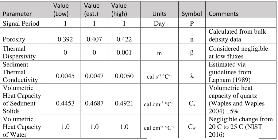
Table 2. VFLUX parameter inputs and values used for this investigation.

Parameter Value (Low) Value (est.) Value

(high) Units Symbol Comments

Signal Period 1 1 1 Day P

Porosity 0.392 0.407 0.422 n

Calculated from bulk density data

Thermal

Dispersivity 0 0 0.001 m β

Considered negligible at low fluxes

Sediment Thermal

Conductivity 0.0045 0.0047 0.0050 cal s-1 °C-1 λ

Estimated via guidelines from Lapham (1989) Volumetric Heat Capacity of Sediment Solids

0.4453 0.4687 0.4921 cal cm-3_°C-1 _C_s

Volumetric heat capacity of quartz (Waples and Waples 2004) ±5%

Volumetric Heat Capacity of Water

1.0 1.0 1.0 cal cm-3_°C-1 _C_w

Negligible change from 20 C to 25 C (NIST 2016)

3) Following the resampling and filtering, VFLUX 2 runs the dynamic harmonic regression (DHR) program from the CAPTAIN toolbox (Young et al. 1999, Young 2006)) to filter temperature time series. Unlike a bandpass filter, DHR permits sub-cycle calculation of water flux via stochastic, time variable parameters that describe how the amplitudes and phases of the time series components vary with time. Using these time-varying parameters, it is possible to calculate the amplitude and phase at different moments in time along a

(29)

sensor. Either or both of Ar and ∆Φ can be utilized in calculating water flux (Hatch et al. 2006; McCallum et al. 2012; Luce et al. 2013).

4) Using Ar and ∆Φ, VFLUX 2 was used to produce hourly-scale estimates of water flux (explained below), thermal diffusivity, and sensor spacing (the latter are useful for quality control). A few options are available to solve for water flux; in this work we relied on the amplitude ratio method developed by Hatch et al. (2006). Ar-derived fluxes tend to be prone to lower errors under upwelling conditions (upward groundwater flow) than ∆Φ-derived water fluxes, and it is common for field-based thermal modeling investigations to exclusively report water fluxes derived from the Ar method (e.g., Lautz and Ribaudo 2012; Daniluk et al. 2013; Rosenberry et al. 2016). Furthermore, if there are issues with proper characterization of ∆Φ, then combined Ar and ∆Φ methods can be unreliable. For example, Irvine et al. (2017) found increased root mean square error for water fluxes calculated via combined Ar and ∆Φ methods for upwelling water fluxes greater than 1 m/d.

When the sediment properties above the shallower temperature sensor are the same as those between the two temperature sensors in a profile, the amplitude ratio can be

expressed as (Hatch et al. 2006):

Ar= exp [

∆Z

2K_e(v − √ α + v2

2 )] (4 – 3)

where

α = √v4 _{+ (8π ∙}Ke

P)

2

(30)

P represents the period of the diurnal signal (86400 s). Equation 4-3 can be rearranged to solve for v, the thermal front velocity (which is then multiplied by C/Cw to give vf, the specific discharge of water, as v(C/Cw)):

v = 2Ke

∆z ln(Ar) + √ α + v2

2 (4 – 5)

Ke is not on Table 2 as a user-input into vflux.m, but vflux.m calculates Ke from user-selected values of λ and C input into vflux.m prior to calculating vf. Equation 4-5 must be solved iteratively for a value of v that satisfies the equation because v is present on both sides of the equation. In VFLUX 2, equation (4-5) is rearranged such that v is only on one side of the equation and the “fzero” command is used to solve for the value of v closest to v=0.

Once vf calculations were made using Ar, I used VFLUX 2 to produce estimates of thermal diffusivity (which are separate from the Ke used in equation 4-5 and independent of user-input λ and C) and sensor spacing using methods that incorporate Ar and ∆Φ (explained below). Time series of thermal diffusivity were used as a quality control to find periods where estimates of vf were potentially unreliable (as indicated by unrealistically high or low Ke) and to adjust vf using the vflux_qar_opt addon (described in step 5 below). Sensor spacing (Δz) estimates were also used as a quality control to compare calculations to the known Δz (7 cm).

I used solutions from Luce et al. (2013) that incorporate Ar and ∆Φ data

(31)

Ke = ∆z

2_ω

∆Φ2₍1

ɳ + ɳ)

(4 – 6)

where η = -ln(Ar) / ∆Φ and ω is the angular frequency for the diurnal frequency (2π/P). I

generated a time series of thermal diffusivity estimates by using equation 4-6 at two hour

intervals to identify moments in time where the diurnal signal is not stationary due to changing flux conditions (indicated by unrealistic Ke), which constitutes a violation of the assumption of steady flow. When the temperature signal is not stationary, the apparent estimated value of thermal diffusivity can undergo large temporary shifts. The shifts can be used to indicate periods where flux estimates should be viewed cautiously (e.g., McCallum et al. 2012; Irvine et al. 2015b).

The second formula calculates distance between temperature sensors:

∆z = √2 ∗ Ke

ω ∗ √

ln(Ar)2+ ∆Φ2

2η (4 – 7)

As with thermal diffusivity, I generated a time series of ∆z using equation 4-7 at two hour intervals as a means of identifying periods where vf estimates could have been prone to higher uncertainty. Sensor spacing is known between pairs of temperature sensors, and if calculations of estimated sensor spacing substantially deviate from the true known sensor spacing, it can indicate moments where vf results are unreliable.

(32)

5) Erroneous selection of values for volumetric heat capacity and thermal

conductivity can introduce error into vf and ∆z calculation by affecting Ke and C/Cw. I used a recent add-on developed for VFLUX 2, vflux_qar_opt (Irvine et al. 2017), to modify

calculations of vf and ∆z. The modified vf and ∆z will be referred to as “optimized”. The vflux_qar_opt function was run separately from the vflux function (from steps 2-4 above).

The vflux_qar_opt function was run after vflux, using the output of the vflux function (the MATLAB structure from the end of step 4), and user-selected values for Ke, Cs, Cw, and porosity as inputs. I input the average Ke from step 4 into vflux_qar_opt, while Cs, Cw, and porosity were unaltered. When vflux_qar_opt is run, it recalculates vf and ∆z (from equations 4-5 and 4-7) and produces separate time series of these parameters. These recalculated vf and ∆z are referred to as being optimized because they are calculated using a value of Ke

calculated for the sediment between the temperature sensors rather than a value estimated from literature.

vflux_qar_opt also calculates and produces a time series of the thermal Peclet number (Pet), a dimensionless parameter that quantifies the relative contributions of conductive and advective heat transfer. Rau et al. (2012) found that for uniform coarse sand, thermal dispersivity (β) can be neglected when Pet_{< 0.5. I used the time series of Pe}t_{to check} whether neglecting β could have had an appreciable impact on estimates of vf. This formula for Pet is from equations 25 and 52 from Luce et al. (2013):

Pet = 2 − η

(33)

The output of vflux_qar_opt is a single MATLAB structure, which contains the same information as the vflux structure array from the prior step, along with modified calculations of vf and ∆z, and a time series of Pet, among other things.

4.5 Groundwater Sampling and Analysis

Piezomanometers (Kennedy et al. 2007) were used to collect groundwater samples from the streambed, at points about 20-25 cm laterally from the temperature profilers. Steel piezomanometers were easily pushed into the streambed and groundwater was withdrawn from approximately 17-22 cm below the top of the streambed (the piezomanometer screens were 5 cm long). Thus, the top of the sampling screen was 2 cm deeper than the deeper temperature loggers deployed in the streambed (the latter were 15 cm below the top of the streambed from December 2016 to March 2017). Samples were collected in amber glass volatile organic analysis (VOA) vials containing 25 mg ascorbic acid and 200 mg of maleic acid as preservatives as outlined by EPA method 524.3. Samples were analyzed using gas chromatography/mass spectroscopy (GC/MS) to determine VOC concentration following EPA method 524.3 (Prakash et al. 2009) in the Environmental Engineering Laboratory overseen by Professor Detlef Knappe at NC State University. Samples were collected in pairs, and the mean value of both tested samples was considered to be the VOC

concentration.

Advective VOC flux, fvoc(μg m-2 d-1), was quantified as fvoc = vf[VOC], where brackets indicate VOC concentration (μg L-1). This calculation assumes that the effects of sorption and degradation in the 17 cm between the sampling point and the top of the

(34)

fvoc was quantified every 3-4 days during three time periods, at three locations in the streambed of Hominy Swamp Creek (Table 1).

4.6 Measurement of Soil Thermal Diffusivity and Volumetric Heat Capacity

Due to the importance of finding appropriate values for λ, C, and Ke, these thermal properties were directly measured using a dual-probe heat-pulse technique (Bristow et al. 1994). Six cores of sediment were collected from the upper 5 cm of sediment using a stainless steel ring: two near site 78L-B, two near site 91R, and two in between sites 78L-B and 91R.

A probe consisting of three parallel needles was inserted into each core of sediment. The central needle sent a short-duration heat pulse through the sediment core, while the other two needles recorded temperature at a precisely known distance from the heat source every second. The thermal properties were determined from the observed magnitude of temperature change and the time it took for the peak temperature to be achieved. Temperature in the sediment as a function of distance and time caused by a short-term heat pulse can be expressed as (Bristow et al. 1994):

𝑇(𝑟, 𝑡) = 𝑄

′

4𝜋𝐾_𝑒[𝐸𝑖 (

−𝑟2

4𝐾_𝑒(𝑡 − 𝑡_𝑜)) − 𝐸𝑖 ( −𝑟2

4𝐾_𝑒𝑡)] (4 − 9)

(35)

Taking equation 4-9 and differentiating with respect to time and setting equal to zero produces the equation used to solve for thermal diffusivity from the heat pulse data (Bristow et al. 1994):

𝐾_𝑒 = (𝑟

2

4) (_𝑡 1

𝑚− 𝑡𝑜) − (

1 𝑡_𝑚) ln [_𝑡 𝑡𝑚

𝑚− 𝑡𝑜]

(4 − 10)

where tm is the time it takes for the maximum temperature change at a temperature sensor distance r from the heat source. Volumetric heat capacity was also quantified using the heat pulse data (Bristow et al. 1994):

𝐶 = 𝑞

′

4𝜋𝐾_𝑒∆𝑇_𝑚[𝐸𝑖 (

−𝑟2

4𝐾_𝑒(𝑡_𝑚− 𝑡_𝑜)) − 𝐸𝑖 ( −𝑟2

4𝐾_𝑒𝑡_𝑚)] (4 − 11)

where ∆Tm Is the maximum temperature change recorded at distance r from the heat source.

5. Results and Discussion

5.1 Temperature Time Series

(36)

From Dec. 6, 2016 to Jan 27, 2017, temperature time series at both depths (8 and 15 cm) show little deviation between sites 78L-A and 78L-B, with mean residuals at 8 and 15 cm (temperature at 78L-B minus that at 78L-A) of 0.074 and -0.012°C, respectively. Between sites 78L-B and 91R, the mean residuals at 8 and 15 cm (temperature at 78L-B minus that at 91R) were -0.129 and -0.473°C, respectively. Greater upward groundwater discharge (“upwelling”) at site 91R relative to site 78L-B (see Section 5.2 below) means that

the mean annual temperature will be encountered at a shallower depth at site 91R. Since this work was done in the winter, the streambed should be colder than the mean annual

temperature and would explain why 78L-B is typically colder at both depths. During the summer, the streambed is warmer than the mean annual temperature, and temperature data from 7/22/2016 to 8/01/2016 show warmer temperatures (0.065°C on average) at site 62LC, a site of weaker upwelling from 3-10 cm deep (Table 3) than site 54L where vf was greater.

(37)

5.2 Water Flux

From late July to early October, water fluxes at the seven measurement sites were between 0.8 m/d (upward flow) and -0.8 m/d (downward flow) (Figs. 5.2-5.8). For 6 of the 7 sites mean water flux was downward in the streambed depth interval 10-17 cm, but mean flux was upward in the depth interval 3-10 cm at 5 of the 7 sites (Table 3). Inconsistency in water flux direction with depth has been encountered in prior heat-tracing work (e.g. Briggs et al. 2012; Gordon et al. 2013). The changes in flux direction with depth may be related to shallow hyporheic flow paths. For instance, in a set of flume experiments, Norman and Cardenas (2014) demonstrated that hyporheic flow can affect the thermal regime of sediment, even with a flat bed.

(38)

Figure 5.2: Water flux (specific discharge) at site 54L. Water fluxes were calculated using the vflux_qar_opt addon (Irvine et al. 2017) in VFLUX 2. Positive values indicate upward flux.

(39)

Figure 5.4: Water flux (specific discharge) at site 46RC in early August 2016. Water fluxes were calculated using the vflux_qar_opt addon (Irvine et al. 2017) in VFLUX 2. Positive values indicate upward flux.

(40)

Figure 5.6: Water flux (specific discharge) at site 62LC in late September 2016. Water fluxes were calculated using the vflux_qar_opt addon (Irvine et al. 2017) in VFLUX 2. Positive values indicate upward flux.

(41)

Figure 5.8: Water flux (specific discharge) at site 62RC. Water fluxes were calculated using the vflux_qar_opt addon (Irvine et al. 2017) in VFLUX 2. Positive values indicate upward flux.

(42)

(43)

Table 3. Mean and range of vf (m/d) for different sites in HSC from late July 2016 to early March 2017. Streambed depth intervals in which the vf estimates were made (defined by the depths of the temperature sensors) are shown (3-10 cm, 10-17 cm, and 8-15 cm). Standard deviations are shown in parentheses. Positive vf corresponds to upward flow.

7/22/16 - 8/01/16 Mean Optimized vf Range of vf

Profiler Location 3-10 cm deep 10-17 cm deep 3-10 cm deep 10-17 cm deep A 54L 0.23 (0.03) 0.05 (0.01) 0.18 to 0.28 0.03 to 0.06 C 62LC 0.04 (0.03) -0.04 (0.01) -0.001 to 0.100 -0.02 to -0.07

Profiler Location 3-10 cm deep 10-17 cm deep 3-10 cm deep 10-17 cm deep A 46RC 0.10 (0.09) -0.14 (0.08) -0.12 to 0.31 -0.07 to -0.30 D 46LC -0.04 (0.25) -0.21 (0.17) -0.82 to 0.50 -0.65 to 0.11

Profiler Location 3-10 cm deep 10-17 cm deep 3-10 cm deep 10-17 cm deep B 62LC -0.20 (0.17) -0.21 (0.07) -0.57 to 0.03 -0.10 to 0.37 C 46LC 0.11 (0.16) -0.08 (0.08) -0.16 to 0.34 -0.21 to 0.05 D 62RC 0.44 (0.26) -0.12 (0.12) -0.05 to 0.76 -0.32 to 0.05

Profiler Location 8 - 15 cm deep 8 - 15 cm deep

A 78L-A 0.003 (0.07) -0.09 to 0.19

B 78L-B 0.03 (0.10) -0.11 to 0.27

A 91R 0.19 (0.08) 0.04 to 0.37

B 78L-B 0.015 (0.06) -0.13 to 0.12

B 78L-B 0.03 (0.09) -0.13 to 0.32

(44)

vf at 91R was consistently higher than that at 78L-B (mean vf values of 0.19 and 0.015 m/d, respectively), and is consistently upwelling.

These differences in the behavior of water flux between 78L and 91R might be at least partially due to differences in streambed morphology and hyporheic flow. As noted earlier (section 4.2), site 78L was just downstream of a pool, a likely location for initiation of hyporheic circulation by penetration for stream water into the streambed. If variations in the hydraulic forcing for hyporheic circulation occur here, in association with variation in stream discharge, it seems possible that the strength and exact locations of hyporheic circulation may vary over time, perhaps causing the dividing line between upward flow and downward flow to shift back and forth over time on the streambed surface, placing site 78L alternately in upwelling and downwelling areas, as shown in the data.

Broadly speaking, variability in vf (as indicated by its standard deviation) was greatest in the shallow (3-10 cm) pre-hurricane data, and lower in the post-hurricane (8-15 cm) and deeper pre-hurricane (10-17 cm) data.

(45)

cases, e.g., at site 78L (mean fluxes were 0.003 and 0.03 m/day, much lower than the fluxes measured by Nickels at individual moments in June 2015 and January 2016). The thermal modeling techniques used in this study allowed identification of this dynamic behavior in a way that other methods aimed at spatial rather than temporal variation (Nickels 2016) could not.

Over the duration of the project, the installed thermal profilers were exposed to snow and intermittent rain. Examples of precipitation causing increases in water flux are on Fig. 5.11, where there is a surge in water flux following precipitation on December 19, 2016, January 1-3, 2017, and January 6-7, 2017. However, there does not appear to be a clear, consistent response to precipitation. The response of vf, water flux between the stream and groundwater, would depend on whether groundwater or stream water head rose faster in response to the precipitation, which may depend on the intensity and location of

(46)

Figure 5.11: Water flux and daily precipitation at site 78L-B from 12/07/2016 to 3/10/2017. Tick marks represent 00:00 for each day.

In general, changes in flux with depth suggest the possibility of a horizontal

component of water flux, which can produce errors in calculation of vf. Reeves et al. (2016) assessed the effects of nonuniformity in water flux by modeling 3 dimensional nonuniform flow. They found that with vertical vf of 0.04 – 0.05 m/d and horizontal vf ranging from 0.06 – 0.1 m/d, the methods used here to estimate 1-D vertical water flux from temperature data

(47)

modeling techniques under controlled hydraulic heads in three-dimensions and controlled sinusoidal heating) before any comparisons to field data are made.

Large rates of change in vf with time may also be associated with greater uncertainty in estimates of vf. The change in water flux from around Jan. 6th to Jan. 9th at site 78L-B are among the most prominent shifts in water fluxes from all vf time series collected in this work, where the flux shifts from 0.31 to -0.11 m/d over 36 hours (dv/dt = 0.28 m/d per day). Rau et al. (2015) simulated a water change rate of 0.25 m/d per day and water fluxes calculated using temperature time series filtered by DHR had a root mean square error of 0.02 m/d.

Compared to vf produced from estimated thermal parameters (Table 2), optimized fluxes were 0.025 m/d lower on average at 78L-A, 0.018 m/d lower at 78L-B, and 0.071 m/d lower at 91R. These differences are smaller than those found by Irvine et al. (2017) for the same sort of comparison (approx. 0.2 to 0.4 m/d; Figures 4 and 8 in Irvine et al. 2017). Because Ke is proportional to thermal front velocity, the slightly lower optimized fluxes can be attributed to mean Ke obtained from eq. 4-5 being lower than the Ke calculated from the λ and C input into vflux.m (Table 2).

Mean estimated Ke values (Table 4) fall within the range for naturally occurring

sediments (2.16 x 10-2_{to 0.18 m}2 _d-1_{; Lapham 1989). I}_{nputs into vflux.m (Table 2; step 4 in}

(48)

(49)

Table 4. Mean calculated thermal diffusivity (m2_{/d) and sensor spacing (cm) for different sites in HSC from late} July 2016 to early March 2017. Standard deviations are shown in parentheses.

7/22/16 - 8/01/16 Mean Ke Mean Calculated ∆z

3 - 10 cm deep

10 - 17 cm deep A 54L 0.111 (0.007) 0.054 (0.002) 7.0 (0.23) 7.0 (0.13) C 62LC 0.087 (0.003) 0.073 (0.002) 7.0 (0.09) 7.0 (0.09)

3 - 10 cm deep

10 - 17 cm deep A 46RC 0.079 (0.014) 0.035 (0.007) 7.1 (0.57) 7.1 (0.82)

D 46LC 0.149 (0.04) 0.06 (0.02) 7.2 (0.81) 7.3 (1.45)

3 - 10 cm deep

10 - 17 cm deep

B 62LC 0.073 (0.01) 0.076 (0.01) 7.1 (0.68) 7.1 (0.47)

C 46LC 0.087 (0.03) 0.073 (0.01) 7.2 (0.88) 7.1 (0.61)

D 62RC 0.187 (0.15) 0.057 (0.01) 7.9 (1.70) 7.1 (0.01)

A 78L-A 0.055 (0.01) 7.2 (1.13)

B 78L-B 0.055 (0.02) 7.2 (1.17)

A 91R 0.051 (0.01) 7.2 (1.00)

B 78L-B 0.058 (0.01) 7.2 (0.70)

B 78L-B 0.06 (0.01) 7.2 (1.02)

(50)

that, on average, deviate from the mean vf by 0.148, 0.220, and 0.140 m/d at sites 78L-A, 91R, and 78L-B (from 12/07/2016 to 03/07/2017; Figs. 5.12 - 5.14), respectively. Within these confidence intervals, water flux is in both directions, making it difficult to definitively state that water flux was consistently upwelling at site 91R and that water flux shifted between upwelling and downwelling at site 78L.

(51)

Figure 5.13: Monte Carlo analysis of vf at site 78L-B.

Figure 5.14: Monte Carlo analysis of vf at site 91R.

(52)

ranging from -1.20 to -1.09 after March 2nd. A negative peclet number indicates that advection and diffusion operate in opposite directions (Garges and Baehr 1998). For heat transport, this translates to advection and conduction (rather than diffusion) acting in

opposite directions. Rau et al. (2012) found that for uniform coarse sand, thermal dispersivity (β) can be neglected when Pet_{< 0.5, and neglecting β has likely had little to no impact on} flux calculations at 78L-A and 78L-B. At 91R, the impact is less clear.

β is typically neglected (e.g., Keery et al. 2007; Luce et al. 2013) or assigned a value

of 0.001 m (e.g., Hatch et al. 2006; Lautz and Ribaudo 2012; Daniluk et al. 2013). Water fluxes using the VFLUX sensitivity function (vfluxsens.m) for β = 0 m and β = 0.001 m (Fig.

5.15) for site 91R show differences less than 7.4 x 10-3_{m/d with a mean of 3.3 x10}-3_m/d. These small differences suggest that neglecting dispersion has had a minimal effect on estimates vf.

(53)

Errors in sensor spacing can impact the estimation of vertical water flux. To evaluate the impacts of erroneous sensor spacing, I used VFLUX 2 to produce water flux time series using temperature sensor spacings of 6, 6.9, 7.1, and 8 cm and compared them to water flux estimates using a 7-cm sensor spacing as done in this work. 1 cm difference in sensor spacing in either direction produces water fluxes that, on average, differ by 5x10-3 m d-1 from water fluxes calculated using a 7-cm temperature sensor spacing. For 0.1 cm errors in sensor spacing, water fluxes differ by 5x10-4_{m d}-1_{in comparison to 7-cm sensor spacing.}

5.3. VOC Concentration and Flux

VOC concentrations were generally below 3 μg L-1 (with only 5 exceptions among 87 measurements) at all the sites covered in this study (Tables 5 and 6; Figs. 5.16 - 5.17). When high [VOC] values found on January 4th, 2017 at site 78 are considered, benzene, vinyl chloride, and cis-DCE show inflated mean [VOC] (and standard deviations) of 0.04(0.04), 1.44 (3.20) and 1.21 (1.50) μg L-1, respectively; the means and standard deviations in [VOC] in Table 5 exclude the outlier January 4th data. [VOC] and fvoc from 01/04/17 will be

regarded as an outlier from this point forward and are excluded in calculations of mean, standard deviation, coefficient of variation, and linear regression. Nickels (2016) found benzene (<0.03 – 0.13 μg L-1₎_{, vinyl chloride (0.36 – 0.73}_{μg L}-1₎_{, and cis-DCE (0.51 – 0.80}

μg L-1₎_{in stream water. Likewise, two surface water samples collected as part of this study}

found mean benzene, vinyl chloride, and cis-DCE concentrations of 0.13, 0.39, and 0.66 μg

L-1, respectively, on 01/24/17.

(54)

concentration and flux shows the greatest. At site 46LC, benzene had the highest concentration, while vinyl chloride and cis-DCE concentrations were 1-3 orders of magnitude smaller.

(55)

(56)

Table 5. Mean, standard deviation, and coefficient of variation for benzene (BZ), vinyl chloride (VC), and cis-DCE (ccis-DCE) concentrations at both sites. The middle group columns (under Site 78L, 1/31-2/20) is included to compare statistics for sites 78L and 91R over that same time period. NA: not applicable, NM: not measured.

Site Site 78L

(12/07-02/20)

Site 78L (01/31-02/20)

Site 91 R (01/31-02/20)

VOC BZ VC cDCE BZ VC cDCE BZ VC cDCE

[VOC] (μg L-1₎

7-Dec 0.07 0.77 1.41 N/A N/A N/A NM NM NM

9-Dec _0.04 _0.36 _0.89 _N/A _N/A _N/A NM NM NM

20-Dec _0.03 _0.80 _1.04 _N/A _N/A _N/A NM NM NM

4-Jan _0.18 _14.83 _7.46 _N/A _N/A _N/A NM NM NM

13-Jan 0.09 3.89 2.15 N/A N/A N/A NM NM NM

31-Jan 0.01 0.01 0.33 0.01 0.01 0.33 0.01 0.03 0.10

3-Feb 0.01 0.02 0.47 0.01 0.02 0.47 0.01 0.05 0.25

7-Feb 0.01 0.05 0.40 0.01 0.05 0.40 0.01 0.04 0.16

10-Feb 0.03 1.24 0.99 0.03 1.24 0.99 0.01 0.01 0.26

14-Feb 0.01 0.02 0.46 0.01 0.02 0.46 0.01 0.10 0.28

17-Feb 0.02 0.58 0.66 0.02 0.58 0.66 0.02 0.17 0.19

20-Feb 0.02 0.36 0.61 0.02 0.36 0.61 0.04 0.28 0.25

Mean [VOC]

(μg L-1₎ 0.031 0.730 0.891 0.016 0.326 0.560 0.016 0.096 0.213 σ 0.022 0.931 0.441 0.007 0.425 0.205 0.010 0.090 0.060 Coefficient

of Variation 0.700 1.276 0.495 0.464 1.305 0.366 0.668 0.935 0.284

(57)

(2016) at the same point, but benzene was almost entirely absent at both sites and is less abundant at 78L and 91R than at several of the measurement spots studied by Nickels (2016) in Hominy Swamp Creek.

Table 6. VOC concentration and fluxes for benzene, vinyl chloride, and cis-DCE at site 46LC.

Site Site 46LC

VOC BZ VC cDCE

[VOC] (μg L-1₎

27 Sept 2016 5.16 0.16 0.395 30 Sept 2016 16.46 0.05 0.09

fvoc (mg m-2 d-1)

(58)

Table 7. Mean, mean absolute value, standard deviation, and coefficient of variation for benzene, vinyl chloride, and cis-DCE fluxes (mg of VOC per square meter of streambed per day) at sites 78L and 91R. The middle column is included to compare statistics for sites 78L and 91R over the same period. NA: not applicable, NM: not measured.

Site Site 78 L

(12/07-02/20)

Site 78 L (01/31-02/20)

Site 91 R (01/31-02/20)

fvoc (mg m-2 d-1)

7-Dec 1.86E-02 2.05E-01 3.75E-01 N/A N/A N/A NM NM NM

4-Jan 1.80E-02 1.48E+00 7.46E-01 N/A N/A N/A NM NM NM

6-Jan 8.15E-03 3.12E-01 3.12E-01 N/A N/A N/A NM NM NM

13-Jan -6.65E-03 -2.87E-01 -1.59E-01 N/A N/A N/A NM NM NM

17-Jan -2.60E-03 -5.11E-02 -7.45E-02 N/A N/A N/A NM NM NM

31-Jan _2.50E-04 _2.50E-04 _8.25E-03 _2.50E-04 _2.50E-04 _8.25E-03 2.57E-03

1.03E-02 2.57E-02

3-Feb _6.35E-04 _1.27E-03 _2.98E-02 _6.35E-04 _1.27E-03 _2.98E-02 3.06E-03 1.53E-₀₂ 7.64E-02

7-Feb

-6.97E-04 -3.48E-03 -2.79E-02

-6.97E-04 -3.48E-03 -2.79E-02 1.67E-03

6.67E-03 2.67E-02

10-Feb _5.82E-04 _2.41E-02 _1.92E-02 _5.82E-04 _2.41E-02 _1.92E-02 1.05E-03

1.05E-03 2.73E-02

14-Feb

8.08E-04 1.62E-03 3.72E-02 8.08E-04 1.62E-03 3.72E-02 4.80E-03

2.40E-02 6.71E-02

17-Feb _2.55E-04 _7.38E-03 _8.40E-03 _2.55E-04 _7.38E-03 _8.40E-03 5.36E-03

4.56E-02 5.10E-02

20-Feb _-6.13E-04 _-1.10E-02 _-1.87E-02 -6.13E-₀₄ _-1.10E-02 _-1.87E-02 5.40E-03

3.78E-02 3.37E-02

Mean fvoc

(mg m-2_d-1₎ 0.0025 0.0357 0.0641 1.74E-04 0.0029 0.008 3.41E-03

2.01E-02 4.40E-02

Mean |fvoc|

(mg m-2_d-1₎ 0.004 0.073 0.094 5.48E-04 0.007 0.021 0.003 0.02 0.044

σ 0.005 0.119 0.122 0.001 0.010 0.022 0.002 0.015 0.019

Coefficient

(59)

(60)

(61)

Figure 5.20: Water and VOC flux at site 91R. Tick marks represent 01:30:00 of each day.

From 01/31/2017 to 02/20/2017 at 78L-B, fvoc was typically lower in magnitude when compared to fvoc from 12/7/2016 to 1/27/2017, though a two-tailed t-test does not indicate that the means were statistically different. The mean benzene flux was essentially zero, and the mean vinyl chloride and cis-DCE fluxes were an order of magnitude smaller compared to mean fvoc from 12/7/2016-1/27/2017. The period of decreased fvoc also coincides with

decreased mean [VOC] and vf. Over the same period site 91R had higher magnitude fvoc than site 78L-B due to higher magnitude [VOC] and vf, and vf which was also consistently

upwards, while vf at site 78L periodically shifted between upwelling and downwelling. In

(62)

I investigated the correlation of vf against fvoc to begin to address whether vf may be used as a proxy for fvoc. Even though VOC flux and water flux are obviously related (since fvoc = vf[VOC]), linear regression analysis of vf against fvoc could be a useful tool for the prediction of fvoc (if the correlation is strong, meaning [VOC] is relatively constant or is correlated with vf) since gathering high-frequency [VOC] data is more labor intensive than streambed temperature time series. In addition, I also investigated the correlation between the independent variables vf and [VOC].

From 12/07/2016 to 02/20/2017 correlation coefficients at site 78L-B between fvoc and vf were calculated with the outlier from 01/04/2017 removed. Over this timeframe, fvoc shows moderate to strong correlations with vf which are statistically significant at the 95% level (Figures 5.21 – 5.23, Table 8). Even for a shorter subset of these 78 L-B results

(1/31/2017-2/20/2017, the same period covered by data collection at 91R), correlations were significant for benzene and cis-DCE. Thus, after a period of “calibration” (i.e., water and VOC data collection) to determine the regression (such as in this study), there may be potential to estimate fvoc from vf data outside the calibration period, though further work is would be needed to rigorously assess this.

(63)

Figure 5.21: Linear regression of all water and benzene flux results at site 78L-B (except the 1/4/2017 outlier).

Table 8. Correlation coefficients with p values comparing fvoc with water flux and VOC concentration at both sites.

Site 78L-B (12/07/2016 – 02/20/2017)

VOC Flux Correlation with vf

r2_{and p value}

[VOC] Correlation with |vf| r2 and p

value

VOC Flux Correlation with [VOC] r2_{and p value}

Benzene 0.90 (<0.01) 0.44 (0.06) 0.31 (0.20)

Vinyl Chloride 0.77 (<0.01) 0.08 (0.76) -0.20 (0.42)

cis-DCE 0.95 (<0.01) 0.33 (0.16) 0.15 (0.54)

Site 78L-B (01/31/2017 – 02/20/2017)

Benzene 0.94 (0.01) -0.70 (0.08) 0.04 (0.93)

Vinyl Chloride 0.32 (0.49) -0.65 (0.11) 0.78 (0.04)

cis-DCE 0.98 (<0.01) -0.54 (0.21) 0.14 (0.77)

Site 91R (01/31/2017 - 02/20/2017)

Benzene 0.32 (0.49) -0.28 (0.54) 0.78 (0.04)

Vinyl Chloride 0.26 (0.58) -0.12 (0.81) 0.88 (0.01)

(64)

Figure 5.22: Linear regression of all water and vinyl chloride flux results at site 78L-B (except the 1/4/2017 outlier).

(65)

Figure 5.24: Linear regression of all benzene concentration and water flux results at site 78L-B (except the 1/4/2017 outlier).

(66)

The correlations between fvoc and vf at 78L-B suggest that vf could be useful as a proxy for fvoc if it incorporates data over months-long periods. Even for briefer periods, the regression between vf and fvoc was significant, but shows a lower slope and higher y-intercept values (Table 9), which would also be consistent with lower magnitude fvoc from late January to February. Correlations between |vf| and [VOC] were not significant. Despite the effects of autocorrelation, fvoc for benzene and vinyl chloride at site 91R and for vinyl chloride at site 78L from late January to February show weak correlations with vf. One possibility is that [VOC] proportionally varied more than vf for these VOCs over the 3-week period, as correlations between [VOC] and fvoc are both strong and statistically significant for these VOCs. The coefficient of variation in water flux at sites 78L-B and 91R were 160.95% and 35.77%, respectively, when sampled down to the same moments in time [VOC] was

(67)

Table 9. Slope and y-intercept values from linear regression analysis of fvoc versus vf at site 78L-B

Site 78L-B (12/07/2016 – 02/20/2017)

Benzene Vinyl Chloride cis-DCE

Slope y-intercept Slope y-intercept Slope y-intercept

0.047 -0.0005 0.902 -0.023 1.141 -0.0099

Site 78L-B (01/31/2017 – 02/20/2017)

Benzene Vinyl Chloride cis-DCE

Slope y-intercept Slope y-intercept Slope y-intercept

0.0075 0.0018 0.0564 0.0082 0.1934 0.0032

Kennedy et al. (2009) and Nickels (2016) both found that changes in contaminant flux followed changes in water flux. The correlations between fvoc and vf at site 78L-B from 12/07/2016-03/07/2017 demonstrate the value of quantifying vf when characterizing the discharge and offsite migration of VOCs from contaminated aquifers. Additionally, mean [VOC] averaged 2.28 times larger at site 78L-B than at site 91R (range was 0.92 to 3.30 times) from 01/31/2017 to 02/20/2017 (Table 5), but the magnitude of fvoc at site 91R averaged 3.72 times larger than at 78 L-B (range was 2.06 to 6.23 times) (Table 6), which can be attributed to the more consistent, higher magnitude vf at 91R (Table 3). Concentration data alone would not have allowed accurate conclusions about the relative mass transport of VOCs at these two sites. Using thermal modeling techniques in conjunction with

concentration allowed calculation of VOC flux and thus a more meaningful assessment of VOC discharge into the stream, including differences between sites 91R and 78L-B.

(68)

VOC sampling depth (almost twice the depth used in this study) and the streambed surface (in January 2016). Without more specific information regarding biodegradation rates for these chemicals in the streambed of Hominy Swamp Creek at the specific locations and times involved in this study, it’s not possible to definitively state whether biodegradation had an

impact on actual values of VOC flux in the field. In addition, groundwater samples were collected at a greater depth (17-22 cm) than the temperature loggers (17 cm at the deepest), and thus the vf and [VOC] values are slightly displaced from each other vertically. Summer 2016 water flux results suggested vf changing somewhat with depth (though not at sites 78L and 91R, which were not investigated until later in 2016), suggesting the possibility that the actual value of vf in the [VOC] measurement interval (17-22 cm deep) might have been different than the vf computed from the temperature sensors at 8 and 15 cm.

While this project focused on advective fluxes of VOCs through a streambed, VOC fluxes by molecular diffusion were estimated, if only to show how small they would be relative to advective fluxes. Diffusive VOC fluxes (fd) were quantified as fd = nDs(∆C/∆z) where n is porosity (0.407 in the Hominy Swamp streambed; Nickels 2016), Ds is the

effective diffusion coefficient for a solute in the water-filled pores of a porous medium (m2 d -1_{), and ∆C/∆z is the concentration gradient between the sampling depth and top of the}

streambed (μg L-1 m-1). ∆z was taken as the vertical distance from the top of the streambed to the center of the piezomanometer screen (19.5 cm); measured VOC concentrations in

groundwater were taken as ∆C (this effectively assumes the stream water VOC concentration

(69)

Environmental Quality, 2015A), and 1.3x10-5 (Michigan Department of Environmental Quality, 2015B) for benzene, vinyl chloride, and cis-DCE, respectively. The diffusive fluxes of the three VOCs studied were estimated to be 2-4 orders of magnitude smaller than their advective fluxes (Table 10).

Table 10. Diffusive VOC fluxes at site 91R. Effective diffusion coefficient assumed to be 0.5 the coefficient of diffusion in water.

Sites _{Site 78L-B (12/07/2016 – 2/20/2017)} _{Site 91R (1/31/2017 – 2/20/2017)}

VOC BZ VC cDCE BZ VC cDCE

Diffusive fvoc (mg m-2 d-1)

7-Dec 6.80E-06 9.66E-06 1.67E-05 N/A N/A N/A

9-Dec 4.41E-06 4.47E-06 1.05E-05 N/A N/A N/A

13-Dec 2.45E-06 3.69E-06 8.40E-06 N/A N/A N/A

16-Dec 8.95E-07 1.71E-06 8.69E-06 N/A N/A N/A

20-Dec 2.93E-06 9.97E-06 1.23E-05 N/A N/A N/A

30-Dec 3.08E-06 1.10E-05 1.56E-05 N/A N/A N/A

4-Jan 1.84E-05 1.86E-04 8.79E-05 N/A N/A N/A

6-Jan 3.20E-06 1.44E-05 1.35E-05 N/A N/A N/A

13-Jan 9.35E-06 4.88E-05 2.53E-05 N/A N/A N/A

17-Jan 2.66E-06 7.44E-06 1.02E-05 N/A N/A N/A

20-Jan 1.63E-06 2.73E-06 7.04E-06 N/A N/A N/A

24-Jan 5.65E-06 2.93E-05 1.71E-05 N/A N/A N/A

27-Jan 5.24E-06 1.94E-06 7.98E-06 N/A N/A N/A

31-Jan 1.09E-06 1.72E-07 3.92E-06 7.42E-07 4.36E-07 1.17E-06 3-Feb 6.06E-07 2.92E-07 5.57E-06 1.03E-06 6.32E-07 2.94E-06 7-Feb 7.47E-07 6.83E-07 4.74E-06 4.81E-07 4.45E-07 1.94E-06 10-Feb 2.96E-06 1.55E-05 1.17E-05 4.75E-07 1.04E-07 3.09E-06 14-Feb 5.30E-07 2.50E-07 5.43E-06 1.42E-06 1.22E-06 3.30E-06 17-Feb 1.87E-06 7.26E-06 7.76E-06 1.50E-06 2.10E-06 2.24E-06 20-Feb 2.12E-06 4.51E-06 7.14E-06 4.34E-06 3.56E-06 2.93E-06

(70)

be feasible to integrate over time in this way for multiple measurement points, and then integrate over space among the measurement points, to quantify total VOC mass discharge, from aquifer to stream, during the monitoring period. Contrary to what concentration data would suggest, the integrations done here reveal that site 91R, which generally had lower [VOC], discharged 4.2 and 4.4 times the mass of vinyl chloride and cis-DCE than site 78L-B from 1/31/2017 – 2/20/2017. Temporal integrations of VOC discharge like in figures 5.26 and 5.27 can be scaled up to encompass larger areas over longer durations (e.g., a year) to make annual reach-scale assessments of VOC mass discharge.

Table 11. Integrated VOC discharge at sites 78L and 91R, mg of VOC per m2_{of streambed over the 20 day} integration period.

Site Site 78 L-B

(12/07/2016-02/20/2017)

Site 78 L-B (01/31/2017-02/20/2017)

Site 91 R (01/31/2017-02/20/2017)

Integrated Discharge (mg m-2₎

(71)

Figure 5.26: Integrated cis-DCE flux at site 91R.