Division III
STUDY ON NUMERICAL METHOD FOR ESTIMATION OF
SURFACE FAULT DISPLACEMENT
Masataka Sawada1, Kazumoto Haba2, and Muneo Hori3
1 Research Engineer, Civil Engineering Laboratory, CRIEPI, Japan
2 Assistant Manager, Nuclear Facilities Division, Taisei Corporation, Japan 3 Professor, Earthquake Research Institute, The University of Tokyo, Japan
ABSTRACT
A reliable estimation of surface fault displacements is a crucial issue to the safety of nuclear power plant facilities. It is necessary to develop a numerical method for the estimation. In this study, we develop a finite element method to which the following two functions are implemented: 1) a symplectic time integration of explicit scheme to properly conserve the energy of the fault; and 2) a rigorously formulated joint elements of high order. The finite element method is enhanced with parallel computing capability. We carry out verification of the developed method solving simple three-dimensional models of a fault embedded in a rock mass. It is shown that the method is applicable to a model of one million degrees-of-freedom and the time to solution is sufficiently short.
INTRODUCTION
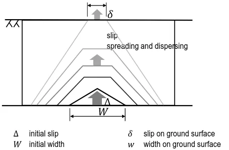
Since the outbreak of huge earthquakes in Taiwan and Turkey in 1999, the concern that surface fault ruptures could damage various infrastructures and buildings has increased. It is necessary to make a reliable estimation of possible displacement (see Figure 1). Indeed, the estimation of fault displacement is a crucial issue for on-site fault assessment in nuclear power plants (NPPs). Numerical simulation for the fault rupture processes is a candidate of such a reliable estimation of fault displacement. There are many numerical simulations of earthquake rupture dynamics for a source fault located in the crust, and the numerical methods used are being applied to the evaluation of surface fault displacement.
An ideal simulation is to compute the whole processes of the rupture from the source fault to the evaluation of surface. However, it is not possible simply because an analysis model is huge in scale and high in spatial resolution, resulting in an acceptable amount of numerical computation. In practice, the following two-step simulation is conducted (JANSI, 2013): 1) evaluate the boundary displacement of an area which includes a target facility, by determining the crust deformation according to the elastic theory of dislocation; and 2) evaluate deformation of the target area using a detailed model of high resolution and fidelity.
A fundamental difficulty in numerical simulation of the fault rupture process is the loss of stability in the initial and boundary value problem to which the numerical analysis is applied. Here, stability means that a solution does not change when a small disturbance is added to the problem, and the stability loss implies drastic change in the solution induced by small disturbance (see Figure 2). This mathematical stability loss inherently induces loss of stability in numerical computation. Finest discretization as well as most rigorous algorithms is thus needed to accurately compute such an unstable solution.
Beside for the use of high performance computing for a large scale analysis model, we develop two rigorous algorithms for the fault rupture process and the time integration. A joint element, which accounts for displacement discontinuity of faulting is rigorously formulated, and a modern symplectic integration is adopted for the time integration in order to satisfy energy conservation.
slip
spreading and dispersing
initial slip
initial width slip on ground surfacewidth on ground surface
Figure 1. Spreading and dispersing of a slip on a fault.
Slip-Spring Constant Relation
3 solutions of for
Slip-Traction Relation Dynamic friction
Quasi-static friction
stable stable unstable
Critical slip
Figure 2. Friction characteristics and slip-traction relation
Lagrangian of continuum, and an explicit symplectic integration is presented for the time integration of a Hamiltonian that is converted from the Lagrangian. Finally, a numerical experiment is carried out to verify the developed finite element method, which is enhanced with high performance computing.
USE OF HIGH PERFORMANCE COMPUTING (HPC)
There is a major difficulty in the numerical simulation of the fault rupture process. It requires a large amount of numerical computation in simulating the fault rupture process even though the target are is of the order of a few hundred meters. This is simply because the temporal resolution ought to be in the order of 0.01 sec to capture the dynamic process, and it induces the spatial discretization of 10m if the wave velocity is in the order of 1,000 m/sec. We surely need the use of capability computing of high performance computing (HPC) to numerically simulate the fault rupture process in the second step in order to make reliable estimation of the fault displacement.
PDF of PDF of
worst
expected
We should mention the treatment of uncertainty due to the limitation in the quality and quantity of available relevant data for the underground structure, the stress state, and the source fault dynamics. We may take advantage of capacity or ensemble computing of HPC in order to account for the variability of the fault displacement induced by the uncertainty (see Figure 3).
HAMILTONIAN AND SYMPLECTIC TIME INTEGRATION
Lagrangian and Hamiltonian
Procedures for deriving a Hamiltonian from a Lagrangian are well established; in Figure 4, we provide a schematic view of the procedure used for deriving a Hamiltonian from a Lagrangian of two variables L(v,u) with v=u . Deriving Hamiltonian H required the use of two equations, namely Lagrange’s equation and a consistency condition. Lagrange’s equation was derived from the stationary condition, and the consistency condition was assigned for the two arguments of the Lagrangian, as one argument was the time derivative of the other (see Figure 4). The Hamiltonian was calculated using the Legendre transformation of L, and the time evolution of the system was uniquely defined by canonical equations (Hamilton’s equations). The Hamiltonian represented the total energy of the system: the sum of kinetic and potential energy.
Figure 4. Schematic view of procedures used to derive the Hamiltonian from a given Lagrangian
Symplectic time integration
Symplectic integrations are designed for numerical solutions of canonical equations. A widely used class of symplectic integration is formed using splitting methods. If Hamiltonian H is separable, it can be written in the form
) ( ) ( ) ,
(p u T p F u
H = + . (1)
The canonical equations can be written as follows:
) ( and
)
(p p F u
T
u=∇p =−∇u . (2)
) ( and
)
( 1 1
1 + +
+ = n + ∇p n n = n − ∇u n
n u h T p p p h F u
u , (3)
where h is a time increment, and n is the value of n-th step. We can obtain an approximate solution of un+1 and pn+1 (in this order) only by substitution.
We define the mapping Ph
h U S
S , as
+
∇
p
p
T
h
u
p
u
S
h pU
)
(
:
, (4)
∇
−
)
(
:
u
F
h
p
u
p
u
S
u hP
, (5)For xn defined
T T n T n
n
u
p
x
=
[
,
]
, we can rewrite Eq. (3) more simply using composite mappingh P h U h
E S S
S = as
) (
1 n
h E
n S x
x + = . (6)
Symplectic integrations of higher orders can be obtained as follows. We prepared real numbers
s
b
b
b
1,
2,
,
,b
ˆ
1,
b
ˆ
2,
,
b
ˆ
s (s is natural number) and defined a map Si by substituting bi orb
ˆ
i times h inthe
S
Eh mapping as follows:h b P h b U i i i
S
S
S
=
ˆ . (7)We defined the scheme from xn to xn+1 by using Si as a component as ) (
)
( 2 1
1 S x S S S S
xn+ = h n h = s . (8)
We implemented the following two methods into a parallel FEM program. 1) The Verlet method was a second-order integration of Eq. (2) with s = 2:
. 2 1 ˆ , 2 1 ˆ , 1 , 0 2 1 2 1 = = = = b b b b (9)
2) The third-order symplectic integration (s = 3) discovered by Ruth (1983) was given by
. 1 ˆ , 3 2 ˆ , 3 2 ˆ , 24 1 , 4 3 , 24 7 3 2 1 3 2 1 = − = = − = = = b b b b b b (10)
Simple spring problem
We investigated the efficiency of the symplectic time integration compared to the Newmark β method. The Newmark β method is a widely used implicit time-integration method that is often used with the Newton–Raphson method. We solved the simple spring model shown in Figure 5. The spring coefficient k has nonlinearity similar to that shown in Figure 2. For the condition u≤ ucr, the canonical equations were derived as follows:
f u C u k p m p u k 2 2
2 0 + 2 +
− = =
, (11)
Figure 5. Simple spring model
The parameter values for the proposed model were m = 1.0 kg, f = 0.4 N, k0 = 0.75 N/m, and Ck = 0.25 N. The maximum relative displacement was obtained from the following equation:
− −
= 2
0 0
max
3 16 1 1 4
3
k fC C
k
u k
k
. (12)
In the graphs in Figure 6, we normalized the relative displacement u by umax = 1.737652 m and the elapsed time by the period t =8.265s, which was obtained by solving the following equation in
Mathematica:
f u C u k u
m 2 2 k 2
2
0 + +
− =
, (13)
Eq. (13) is equivalent to the canonical equations (10).
(1) Newmark βmethod (2) Symplectic integration (s= 2)
Figure 6. Progression of the relative displacement
The parameters of the Newmark β method were β = 0.25 and γ = 0.5. We adopted second-order symplectic integration (s = 2) so that the order of convergence was the same as the Newmark β method. Several cases were calculated with different time steps of 1/10, 1/20, 1/50, 1/100, 1/200, 1/500, and 1/1000 of the period t =8.265s.
Figure 6 shows the progression of the relative displacement from the cases of h=t/1000, t/100, and t/10. In both the Newmark β method and symplectic integration, the calculated amplitude and period were very good, except for the case with maximum time step (h=t/10).
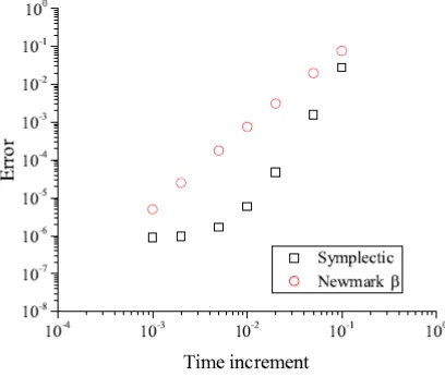
Figure 7 shows the relationship between the error of the solution and the size of the time step. We defined the error as the difference of normalized relative displacement from the analytical solution (zero) after one period. Second-order convergence was obtained from the Newmark β method. The error in the
symplectic integration method was smaller than that in the Newmark β method. Moreover, the
convergence rate was faster in the symplectic integration method than the Newmark β method. Thus, the result from the proposed symplectic integration method was better than that of the Newmark β method, which is a widely used implicit method.
FINITE-ELEMENT METHOD FOR THE FAULT-DISPLACEMENT PROBLEM
We have implemented a rigorous joint element and symplectic time integration method with Hamiltonian formulation into an open-source parallel FEM program FrontISTR (Okuda, 2017) to develop a numerical tool for fault displacement problems.
Nonlinear spring model on faults
Sawada et al. (2017) proposed a rigorous joint element in which the element stiffness matrix of the joint element was derived from the Lagrangian on the discontinuity surface. We implemented the joint element with a nonlinear spring model to represent the fault movement. The spring coefficient per unit area (shear stiffness) κ could be described by the following function of slip u:
>
≤
−
−
=
)
(
)
(
)
(
0 0
cr d
cr cr
d
u
u
u
u
u
u
u
κ
κ
κ
κ
κ
, (14)where κ0 was the quasi-static shear stiffness (initial shear stiffness), κd was the dynamic shear stiffness (final shear stiffness), and ucr was the critical slip (see Figure 2). In dynamic simulations, the slip trajectory utraj was used in place of slip u. Note that we did not use any sliders or dashpots in κ.
Hamiltonian for finite-element method
The Lagrangian has typically been used to formulate FEM, but the Hamiltonian can be expected to work in the formulation as well. In this subsection, we describe a continuum Hamiltonian and a canonical equation for FEM. Hori et al. provided a rigorous derivation of a Hamiltonian from a given Lagrangian of solid continuum. We started from the case that the density of a continuum Lagrangian, denoted by l, was given for a continuum V. Here, l was assumed to be a function of the velocity vector and strain tensor, denoted by v and ε, respectively. In terms of the displacement vector, u(x, t) with x and t being a point and time, respectively, v and ε could be expressed as
{ }
(
,
)
sym
)
,
(
and
)
,
(
)
,
(
x
t
u
x
t
ε
x
t
u
x
t
v
=
=
∇
, (15)∫
=
V
l
dv
L
[
v
,
ε
]
(
v
,
ε
)
. (16)Here, a square bracket means that L is a functional for a vector function and a tensor function, while a parenthesis (or a round bracket) means that l is a function of a vector and a tensor; the same symbol v and
ε are used in L and l for simplicity.
We considered the simplest case when V was linearly elastic. In this case, the continuum Lagrangian density was explicitly expressed with a Cartesian coordinate system and index notation as
kl ij ijkl j
iv c
v
l
ρ
ε
ε
2 1 2 1 ) ,
(v ε = − , (17)
whereρ was the density and c was the elasticity tensor.
To derive the FEM for Hamiltonian, we used a discretized displacement function of the following form:
∑
=
∗)
(
)
(
)
,
(
x
u
x
u
t
αt
ξ
α , (18)where uα was a displacement vector of the α-th node and ξα was an associated shape (or interpolation) function. For a given continuum Lagrangian density, we have
∫
∗∗
=
V
l
dv
L
[{
v
α},
{
u
α}]
({
v
α},
{
u
α})
, (19)with vα =uαand
l
∗=
l
(
∑
v
αξ
α,
∑
sym
{
u
α⊗
∇
ξ
α}
)
. Defining a new variable asp
α=
∂
L
∗∂
v
α , which was the momentum of the α-th node, we derived a continuum Hamiltonian from L* as}]
{
},
[{
}]
{
},
[{
p
αu
αv
αp
α ∗v
αu
α∗
=
∑
⋅
−
L
H
. (20)The canonical equation of this H* was
∂
∂
∂
∂
−
=
∗ ∗ α α α αp
u
u
p
H
H
. (21)
For simplicity, we assumed that the derivatives of H* were given as a linear combination of its arguments,
uβ and pβ, i.e.,
∑
∑
=
∂
∂
=
∂
∂
∗ ∗ j j ij i j j ij ip
K
p
H
u
R
u
H
, ,and
β β αβ α β β αβα , (22)
where Rijαβ = ∂H*2/∂uiα∂ujβ and Kijαβ = ∂H*2/∂piα∂pjβ. We made two vectors, [u] and [p], by arranging uiα and piα, respectively, and we similarly made two matrices, [R] and [K], by arranging Rijαβ and Kijαβ, respectively. In terms of these vectors and matrices, the continuum Hamiltonian of FEM could be expressed as ] ][ [ ] [ 2 1 ] ][ [ ] [ 2 1 u K u p R p
H∗ = T + T , (23)
where superscript T stands for the transpose. The canonical equation became
] ][ [ ] [ and ] ][ [ ]
[p =− K u u = R p . (24)
Note that [K] was the stiffness matrix and that [R] was the inverse of mass matrix [M]; [K] and [M] were constructed as follows:
∫
∫
=
=
V T V Tdv
N
N
M
dv
B
D
B
K
]
[
]
[
][
]
and
[
]
[
]
[
]
[
ρ
. (25)where [B] was a B matrix, [D] was a matrix of elastic constants, ρ was the density, and [N] was a matrix of the shape function. We used the lumped mass matrix in this simulation. These matrices were identical to those used in ordinary FEM.
∫
+ +
= ∗
t j
s T T
d u K u u K u p
R p
H [ ] [ ][ ] [ ][ ][ ]
τ
2 1 ] ][ [ ] [ 2 1
, (26)
where [Ks] was a stiffness matrix of solid elements and [Kj] was a stiffness matrix of joint elements. While we considered nonlinearity of the joint elements, we applied only linear elastic materials to the solid elements in this study. The canonical equation became
] ][ [ ] [ and ] ])[ [ ] ([ ]
[p =− Ks + Kj u u = R p . (27)
APPLICATION OF THE DEVELOPED METHOD
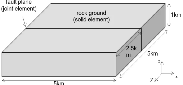
We applied the developed FrontISTR code to a test simulation. We modeled a 5 km × 5 km × 1 km domain of ground that included a vertical fault plane. Figure 8 shows a schematic view of the model. In the first step, our target number of degrees-of-freedom was less than 1,000,000. The model consisted of 1000 second-order triangle elements for the fault, 150,000 second-order tetrahedral elements, 216,342 nodes, and 649,026 degrees-of-freedom.
5km
5km
1km rock ground
(solid element) fault plane
(joint element)
2.5k m
x y
z
Figure 8. Model for the test simulation
1.25km 2.5km 1.25km 1.0m
on the fault plane ignore 0 [m]
forced displacement
x z
Figure 9. Slip distribution forcibly applied on the bottom of the fault
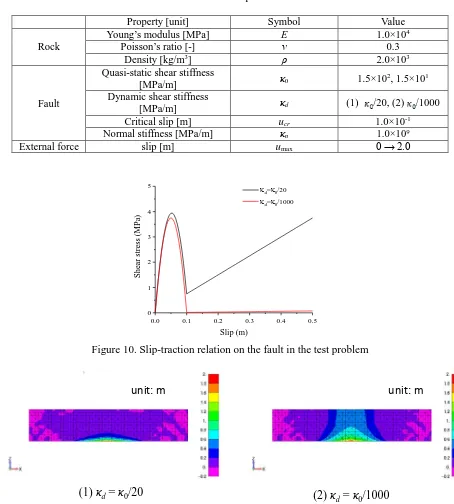
Table 1: Material parameters
Property [unit] Symbol Value
Rock
Young’s modulus [MPa] E 1.0×10⁴
Poisson’s ratio [-] ν 0.3
Density [kg/m3] ρ 2.0×10³
Fault
Quasi-static shear stiffness
[MPa/m] κ0 1.5×10
2, 1.5×101
Dynamic shear stiffness
[MPa/m] κd (1) /20, (2) /1000
Critical slip [m] ucr 1.0×10⁻¹
Normal stiffness [MPa/m] κn 1.0×10⁹
External force slip [m] umax 0 → 2.0
0.0 0.1 0.2 0.3 0.4 0.5
0 1 2 3 4 5
She
ar st
re
ss (M
Pa
)
Slip (m)
κd=κ0/20
κd=κ0/1000
Figure 10. Slip-traction relation on the fault in the test problem
unit: m unit: m
(1) κd= κ0/20 (2) κ
d= κ0/1000
Figure 11. Slip distribution on the fault (t = 3 s)
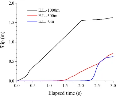
Figure 11 shows the contour of the slip distribution at t = 3 s on the fault plane. In case (1), the slip did not propagate after the input slip was given until t = 2 s. In case (2), on the other hand, the slip propagated and reached the ground surface, and the surface slip was up to 0.6 m.
0.0 0.5 1.0 1.5 2.0 2.5 3.0 0.0
0.5 1.0 1.5 2.0
Sl
ip (m
)
Elapsed time (s)
E.L.-1000m E.L.-500m E.L.+0m
Figure 12. Slip progression at three depths (κd = κ0/1000)
SUMMARY
We proposed a numerical method utilizing Hamiltonian and symplectic time integration, which provided energy conservation and an explicit expression of the time derivative of physical quantities. We conducted a numerical test using a simple model and demonstrated the advantages of the proposed method. A parallel computing FEM program was developed with rigorous joint element and symplectic time integration with Hamiltonian formulation, and this program was applied to a three-dimensional fault displacement model. It is shown that the method is applicable to a model of one million degrees-of-freedom.
ACKNOWLEDGMENT
This study is supported by the commissioned projects from Agency for Natural Resources and Energy, Ministry of Economy, Trade and Industry, JAPAN.
REFERENCES
Hori, M., Wijerathne, L., Riaz, R. and Ichimura, T. “Rigorous derivation of Hamiltonian from Lagrangian for solid continuum,” Journal of JSCE. (under review)
Okuda, H. FrontISTR ver.4.5, http://www.multi.k.u-tokyo.ac.jp/FrontISTR/files/FISTRv4.5E.pdf,
retrieved 14 May 2017.
On-site Fault Assessment Method Review Committee of Japan Nuclear Safety Institute (JANSI) (2013).
Assessment Methods for Nuclear Power Plant against Fault Displacement, JANSI-FDE-03, Japan. Ruth, R. D. (1983). “A canonical integration technique,” Nuclear Science, IEEE Trans. on. NS-30(4)
2669-2671.