Robustness in Latent Variable Models

(1)

Abstract

HUANG, XIANZHENG. Robustness in Latent Variable Models. (Under the direction of Dr. Marie Davidian and Dr. Leonard A. Stefanski.)

Statistical models involving latent variables are widely used in many areas of applications, such as biomedical science and social science. When likelihood-based parametric inferential methods are used to make statistical inference, certain distri-butional assumptions on the latent variables are often invoked. As latent variables are not observable, parametric assumptions on the latent variables cannot be veri-fied directly using observed data. Even though semiparametric and nonparametric approaches have been developed to avoid making strong assumptions on the latent variables, parametric inferential approaches are still more appealing in many situa-tions in terms of consistency and efficiency in estimation, and computational burden. The goals of our study are to gain insight into the sensitivity of statistical inference to model assumptions on latent variables, and to develop methods for diagnosing latent-model misspecification to enable one to reveal whether the parametric infer-ence is robust under certain latent-model assumptions. We refer to such robustness as latent-model robustness.

(2)

(3)

Robustness in Latent Variable Models

by

XIANZHENG HUANG

A dissertation submitted to the Graduate Faculty of North Carolina State University

in partial fulfillment of the requirements for the Degree of

Doctor of Philosophy

STATISTICS

Raleigh 2006

APPROVED BY:

Dr. Marie Davidian Dr. Leonard A. Stefanski

Co-Chair of Advisory Comittee Co-Chair of Advisory Comittee

(4)

To those who care about me

as a daughter, sister, student,

or just as a friend,

(5)

Biography

(6)

Acknowledgements

I was once told that most of the things happen to me result from what I choose. If I choose to be happy, happiness will come to me in one way or the other. If I choose to stay depressed, even the funniest clown in the world will not make me laugh. I do not know if it is true. But there are a few things that I do not think I could ever choose. My dear parents are among them. Yet having such parents is what I feel most fortunate for. They equipped me with the belief that life is more worth living if one has dreams and a strong will to make them come true. Then they set me free and let me fly as far as I want, while believing in that I can make wise choices and I will not settle for less in what I pursue. Their support and faith in me are among those key forces without which I might not be able to go this far on my journey.

(7)

List of Tables

4.1 Values ofT∗

1,1 andT

∗

1,2 assessing robustness of the regression parameter

estimates when λ= 0 and λ= 3 under three ways of modeling for the simulated data used in Example 4.2. Correspondingp-values are given in the parentheses. . . 40 4.2 Values of T∗

1,1 and T

∗

1,2 assessing robustness of the conditional score

estimates and MLEs for the regression parameter under three ways of modeling when λ = 0 and λ = 3 for the simulated data used in Example 4.3. Correspondingp-values are given in the parentheses. . . 40 4.3 Rejection rates (proportion of 100 data sets with_|T∗

1,·|>1.96) in testing robustness of the estimates using T∗

1,1 and T

∗

1,2 for β0 and β1,

respec-tively, whenλ varies from 0 to 3 under three ways of modeling for the simulated data. Numbers in the parentheses are estimated standard errors of the rejection rates. . . 40 4.4 Values ofT∗

1,1 andT

∗

estimates when λ= 0 and λ= 3 under three ways of modeling for the Framingham data. Corresponding p-values are given in the parentheses. 40

5.1 Values ofT∗

1,d (d=1, 2, 3) used to assess the changes inbθ

(c)

B (λ),bθ

(m)

B (λ),

b

θ(Bn)(λ), and bθ

(s)

B (λ), as λ increases from 0 to 2 corresponding to the

simulation in Example 5.1 and Figure 5.1 (a). Correspondingp-values are in the parentheses. . . 61 5.2 Values ofT∗

1,d (d=1, 2, 3) used to assess changes inbθ

(c)

B (λ),bθ

(m)

B (λ), and

b

θ(Bn)(λ) as λ increases from 0 to 2 for the SWAN data. Corresponding

(10)

List of Figures

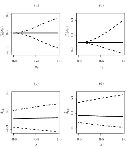
2.1 Figures (a)–(b) illustrate Example 2.1, plots of β0(σU) and β1(σU) for

assumed model N(τ(a)_{, τ}(a)_{) and three true} _X _{distributions,} _N_(1,₁₎

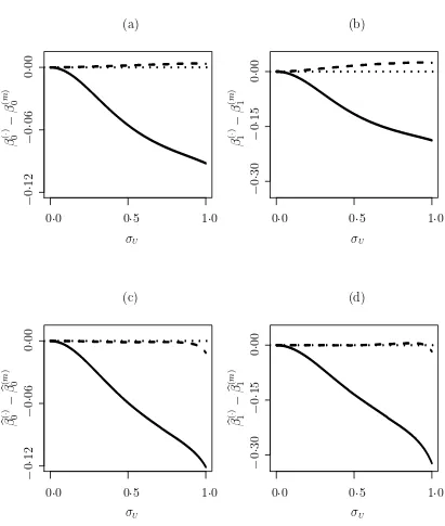
(solid line),N(0_·5,1) (dashed line) and N(1_·5,1) (dashed-dotted line); (c)–(d) single-sample remeasurement versions of (a)–(b) as described in Example 4.1. . . 22 2.2 Plots for Example 2.2 with Y_|X linear-probit. (a)–(b), θ(n)_(σ

U)−

θ(m)_(σ

U) andθ(s)(σU)−θ(m)(σU); (c)–(d) Monte-Carlo estimates based

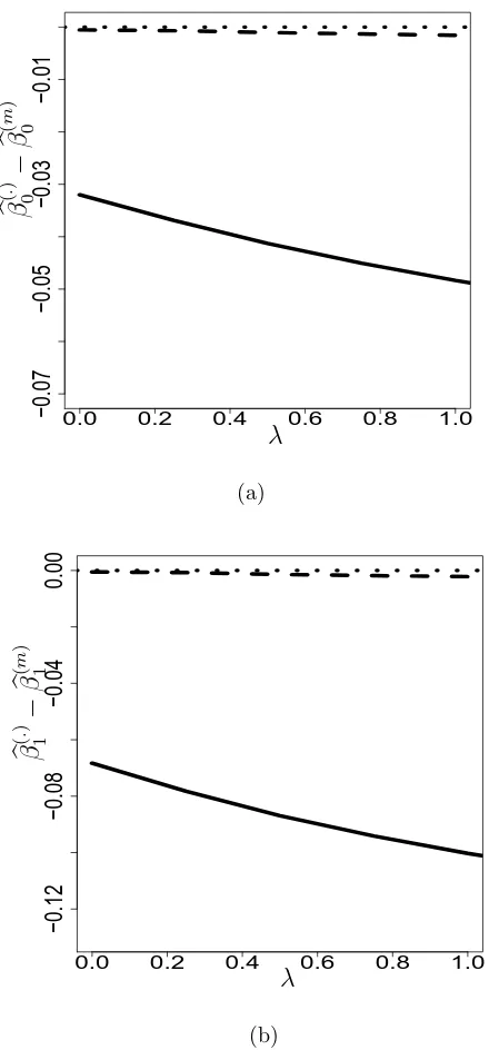
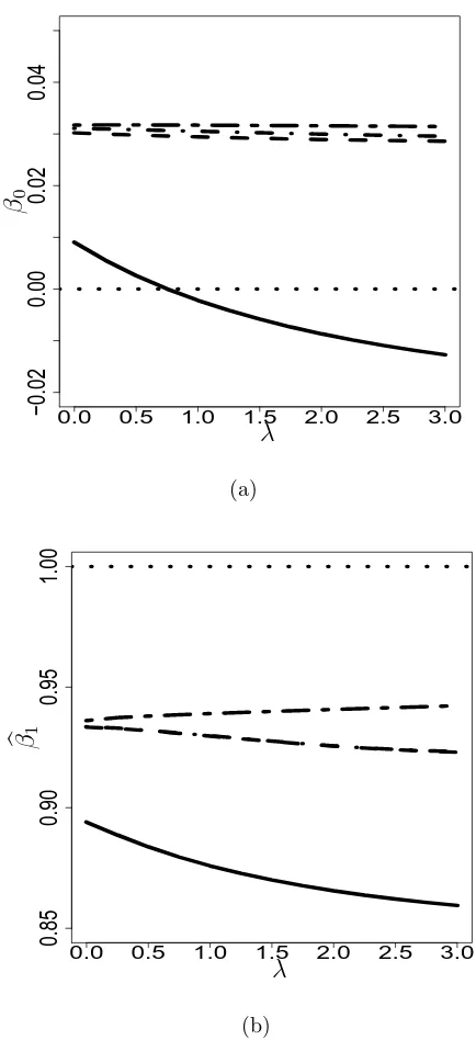
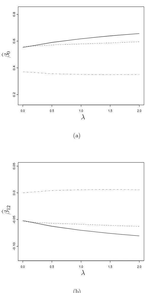
on 100 replicates, of finite-sample, n = 500, version of (a)–(b). The solid line and the dashed line correspond to the normal modelling and seminonparametric modelling, respectively. The dotted line is the ref-erence line. . . 23 4.1 Deviations from the MLEs resulting from the mixture-normal modeling

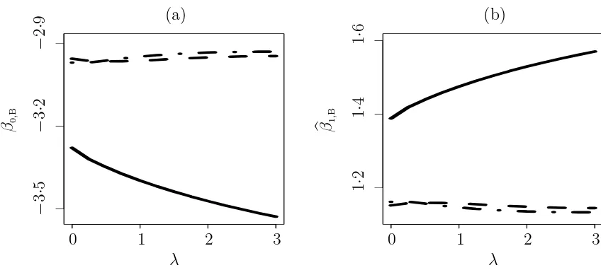
when modeling X as normal and SNP, Example 4.2; (a) corresponds toβb0,B; (b) corresponds to βb1,B. The correspondence of the line types

and ways of modeling is the same as used in Figure 2.2. . . 41 4.2 MLEs under the three assumed models for X and conditional score

estimates versusλ, Example 4.3; (a) corresponds to βb0,B and βb0,∗; (b) corresponds to βb1,B and βb1,∗. True values of β0 and β1 are marked

by the dotted reference lines. Line types used for assumed models are identical to those used in Figure 2.2. The long-short-dash line corresponds to the conditional score estimates. . . 42 4.3 θb(Bn) (solid line), θb

(s)

B (dashed line), and θb

(m)

(11)

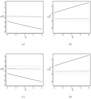
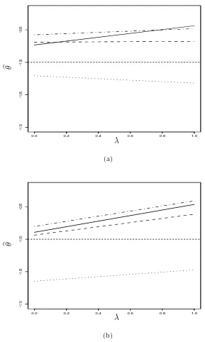
5.1 Plots (a) and (b) show MLE’s assuming mixture BVN, BVN, and SNP random effects, and CSE’s as function of λ obtained at Step 3 of re-measurement method with B = 50 to one “observed” data set. Plots (c) and (d) show averages of N = 30 sets of estimates plotted in (a) and (b) forN = 30 MC replications. Only the plots of the first two re-gression parameters,β0 andβ11, are shown. The line types forbθ

(c)

B (λ),

b

θ_B(m)(λ),bθ_B(n)(λ), andbθ(_Bs)(λ) are dash-multiple-dotted line, dash-dotted line, solid line, and dashed line, respectively. Horizontal lines are ref-erence lines at the true values,β0 =−2 and β11= 1. . . 62

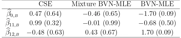
5.2 Plot (a) depicts CSEs and MLEs obtained at Step 2* of remeasurement method withB = 30 whenαi is modeled as MixBVN, BVN, and SNP,

forθ atλ=0, 1. Plot (b) shows the average ofN = 50 sets of estimates ploted in (a) resulting fromN = 50 MC replications. The dotted line is for CSE, the dashed line, solid line, and dash-dotted line are for MLE assuming mixture BVN, BVN, and first-order SNP random effects, respectively. The horizontal line is the reference line at the true θ valueθ =₋1. . . 63 5.3 Plots of MLE’s corresponding to mixture BVN and BVN modeling,

b

θ(Bm), bθ

(n)

B , and CSE, bθ

(c)

B , obtained at Step 3 with B = 50 as functions

of λ, using SWAN data. Line types for θb(Bc)(λ), θb

(m)

B (λ), and θb

(n)

B (λ)

(12)

Chapter 1 Introduction and Models

1.1 Introduction

Models involving unobservable latent quantities are widely used in a host of ap-plications. One example is the structural measurement error models where the latent variable is the true value of a mismeasured regression predictor (Carroll et al., 1995, sec. 1.2). Another example is the so-called “joint” models in which the longitudi-nal response and endpoint are linked through shared dependence on latent random effects (Henderson et al., 2000; Tsiatis and Davidian, 2004). These joint models can be viewed as generalizations of structural measurement error models. Following Car-roll et al. (1995, sec. 1.2), we refer to models involving unobservable random latent variables as structural models.

(13)

in-ference, although some recent empirical studies have exhibited striking robustness to the assumption on the latent variable (Song et al., 2002). The data analyst faces the difficulty that the extent to which inference may be sensitive to the choice of model for unobservable latent variables is not known in a given problem. Techniques for studying and diagnosing robustness in these models would thus be invaluable. We present a framework for assessing model robustness in a class of structural latent variable models.

We first focus on the particular subclass of structural measurement error models, and propose practical strategies for diagnosing misspecification of the model for the true predictor, the latent variable for this subclass. We then adapt the methods to more general and complicated structural latent variable models, namely joint models. To illustrate the proposed methods in the context of different structural latent variable models, we demonstrate the methods using analytical examples, simulated data, and data sets from several medical studies where these models are entertained.

(14)

1.2 Structural Measurement Error Models

We consider the so-called classical measurement error model. Let Y be the response; Xq×1 and Wq×1 be the true and observed predictor, respectively; and

W =X +U, where Uq×1 is nondifferential measurement error (Carroll et al. 1995, Section 1.6) that follows a multivariate normal N(0,σ2

U) with σ

2

U known. In practice

when σ2

U is unknown but there are replicated measures on W, estimating σ

2

U adds

little variation or complexity in implementing the proposed methods. Assuming the conditional density of Y given X = x is fY|X(y|x;θ), the joint density of (Y,W)

given X =x is

fY,W_|X(y,w|x;θ) =fY|X(y|x;θ)fW_|X(w|x;σ

2

U), (1.1)

where the conditional density ofWgivenX,fW|X(w|x;σ2U), is the N(x, σ

2

U) density.

To focus on the choice of model for X, we assume the densities in (1.1) are known up to θp×₁. Inference onθ is of central interest.

Denote the independent random pairs, _{Yi,Wi}ni=1, as a realization of the

mea-surement error model, with Wi = Xi+Ui, i = 1, . . . , n. Two ways of viewing the

Xi, i = 1, . . . , n, lead to two types of measurement error models, functional models and structural models (Carroll et al., 1995, sec. 1.2). In a functional model, the Xi

are viewed as unknown parameters, and the likelihood of the observed data based on model (1.1) is

L(θ,X1, . . . ,Xn) = n

Y

i=1

fY,W|X(Yi,Wi|Xi;θ). (1.2)

(15)

that the density of X is fX(a)(x;τ(a)), depending on parameter τ(a),

fY,W(y,w;θ,τ

(a)_{) =}

Z

fY|X(y|x;θ)fW|X(w|x;σ

2

U)f

(a)

X (x;τ

(a)₎_d_x_, _(1.3)

is the modeled marginal density of (Y,W), and the corresponding likelihood is

L(θ,τ(a)) =

n

Y

i=1

fY,W(Y_i,W_i;θ,τ

(a)_). _(1.4)

An example of a situation where such a model is suitable is the analysis of car-diovascular disease outcomes in the Framingham study (Kannel et al., 1986), which followed subjects for development of coronary heart disease (CHD) over several exam periods. An objective is to characterize the relationship between a response, an in-dicator of evidence of CHD at the end of an eight-year follow-up period after the second exam visit, and long-term systolic blood pressure (SBP). One may postulate a structural measurement error model, where the true predictor, long-term SBP, which cannot be measured directly, is viewed as a latent variable with some distribution in the population of subjects, information on which is only available through contami-nated measurements of SBP taken during clinic visits.

Functional modeling makes minimal assumptions on the set of unobserved pre-dictors and thus is generally applicable. However, functional-model inference is usu-ally problematic. Maximizing the functional likelihood (1.2) with respect to θ and

X1, . . . ,Xn is often difficult and seldom results in consistent estimator for θ.

(16)

Whereas historically, functional models and functional-model methods have been studied more than structural models and methods, recent emphasis has been on struc-tural models and methods. The appeal of strucstruc-tural modeling is mainly due to the fact that inference can be based directly on the likelihood (1.4), thereby simplifying estimation relative to that in functional modeling, apart from the numerical problem of evaluating the integral in (1.3). Maximum likelihood estimation also offers the attraction of asymptotic efficiency when the assumed parametric model fX(a)(x;τ(a))

is correct.

A reason often cited for avoiding parametric structural modeling is that misspec-ification of the distributional model for X can result in inconsistent estimators forθ. With regard to robustness of inference on θ to misspecification of this model, semi-parametric modeling methods (Roeder, Carroll, and Lindsay, 1996; Schafer, 2001) and flexible-parametric modeling methods (Carroll, Roeder, and Wasserman, 1999; Richardson, 2002) provide some solutions. However, with respect to simplicity of implementation and efficiency, they can be more like functional methods than para-metric structural methods. Hence, parapara-metric structural modeling is preferable in practice as long as the analyst may be assured that the inferences are insensitive to an incorrect specification of the distributional model.

To study robustness to model specification on X, we assume that measurement error exists with known variance σ2

U(6= 0) and that the unknown density of X is

(17)

of measurement error variance.

1.3 Joint Models

It is often of interest to characterize the association of a primary endpoint and a longitudinal process, as well as the features of the longitudinal process. One popular approach to tackle this dual-task problem is to adopt a regression model for the primary endpoint and a mixed-effect model for the longitudinal process, which are linked through joint dependence on latent random effects. It has been demonstrated in the literature that, with appropriate parametric modeling of the distribution of random effects, joint modeling can gain efficiency and provide insight into underlying features of the longitudinal process. Similar to what is pointed out in Section 1.2, one concern in this approach is the sensitivity of inference on the primary regression parameters to the model assumptions on the random effects.

For definiteness, we study two types of joint models that are of great interest in medical and public health application. The first type is for an error-prone longitudinal response and a primary simple response (Li et al., 2004; Wang et al., 2000). The second type is for an error-prone longitudinal response and a censored time-to-event (Song et al. 2002; Tsiatis and Davidian, 2001, 2004). Hereafter we refer to the first type as a simple-response joint model and the second type as a censored-endpoint joint model. Some common notations used in both joint models are given first.

Leti(= 1, . . . , n) be the subject index, andj(= 1, . . . , mi) be the time index. The

(18)

recorded at times ti = (ti1, . . . , timi)T. The intra-subject errors, Uij for i = 1, . . . , n

and j = 1, . . . , mi, are independent and identically distributed (i.i.d.) as normal with

mean zero and variance σ2

U. Define Ui = (Ui1, . . . , Uimi)

T_{, then} _U

i ∼Nmi(0, σ2UImi),

where Imi is the mi ×mi identity matrix. Let Ω be the vector of all unknown

parameters in the joint model and θ be the vector of primary regression parameters. Inference onθ is of central interest.

In the simple-response joint models, the joint model consists of two component models: a primary regression model relating the responseYiand thep×1 unobservable

explanatory variablesXi with density denoted byfYi|Xi(Yi|Xi;θ); and a mixed-effect

model relating the longitudinal measurements Wi and Xi, the unobserved

subject-specific random effects. We consider a linear mixed model of the formWi =DiXi+

Ui, where Di is an mi ×p (mi > p) design matrix of rank p. It is further assumed

that given Xi, Yi and Wi are independent. Define by fX(ai)(Xi;τ

(a)_{) the density of}

the assumed model for Xi, where τ(a) is the vector of parameters in the assumed

model. In this case, Ω= (θT,τ(a)T_{, σ}2

U)

T_{; and the contribution to the observed-data}

likelihood from subject iis

fYi,Wi(Yi,Wi;Ω) = Z

fYi|Xi(Yi|xi;θ)fWi|Xi(Wi|xi;σ

2

U)f

(a)

X_i(x_i;τ

(a)_)d_x

i, (1.5)

where fWi|Xi(w|xi;σ

2

U) is the density of Nmi(Dixi, σ

2

UImi).

(19)

a proportional hazards model with hazard rate given by

λi(u) = lim h→0h

−₁

P(u_≤Ti < u+h|Ti ≥u, Xi, Fi, Ci,ti)

= λ0(u) exp{βXi(u) +ιFi}, (1.6)

whereλ0(u) is an unspecified baseline hazard function,Xi(u) is the inherent value of

a longitudinal response at timeu,Fi is the value of the time-independent covariate,β

andιare parameters. The observed survival data on subjectiincludeVi = min(Ti, Ci)

and ∆i =I(Ti ≤Ci), whereTi andCi are the (potential) time to event and censoring

time, respectively, and I(_·) is the indicator function. Censoring, covariate errors, and timing of measurements are assumed noninformative. The second component model relates the observed longitudinal measuresWij to the inherent longitudinal measures

Xi(tij), Wij = Xi(tij) +Uij. It is further assumed that Xi(u) depends on a p×1

vector of subject-specific random effects, αi, via the relationship Xi(u) = Di(u)αi,

for instance, whereDi(u) is a 1×pdesign matrix. Define byfα(ai)(αi;τ

(a)_{) the assumed}

model for αi. In this caseΩ= (θT,τ(a)T, λ0, σU2)

T _and _θ_{= (β, ι)}T_{. The contribution}

to the observed-data likelihood from subjecti is

f(Vi,∆i,Wi,ti, Fi;Ω) =

Z

f(Vi,∆i|αi, Fi;θ, λ0)fWi|αi(Wi|αi,ti;σ

2

U)

fα(ai)(αi|Fi;τ

(a)_)d_αi_, _(1.7)

wherefWi|αi(w|αi,ti;σ

2

U) is the density ofNmi(Diαi, σ

2_Imi_{), and assuming the}

haz-ard rate in (1.6),

f(Vi,∆i|αi, Fi;θ, λ0) = [λ0(Vi) exp{βDi(Vi)αi+ιFi}]∆i

exph₋

Z Vi

0

λ0(u) exp{βDi(u)αi+ιFi}du

i

(20)

An example where the simple-response joint model is appropriate is the Study of Women’s Health Across the Nation (SWAN) (Sowers et al., 2003). Two objectives of SWAN study are to characterize the association between the evidence of osteopenia, a binary endpoint, and the underlying hormone patterns over the menstrual cycle in peri-menopausal women, and to understand the underlying hormone patterns of this population, which can only be observed in this study through the longitudinal progesterone levels derived from urine (PDG).

The censored-endpoint joint model is appropriate for data from the AIDS Clinical Trials Group (ACTG) Protocol 175 (Hammer et al., 1996). In this study, more than 2000 HIV-1-infected subjects enrolled between December 1991 and October 1992 were followed for their CD4 counts from week 8, and every 12 weeks thereafter, until November 30, 1994. The “event” defined in this study is a composite of_≥50% decline in CD4, progression to AIDS, or death. It is of interest to study the prognostic value of CD4 counts and its inherent trajectory over time for such a population.

(21)

(22)

the normality assumption on the random effects. Hsieh et al. (2006) investigated this robustness aspect of joint models via simulation and provided a heuristic explanation for this phenomenon.

1.4 A Brief Tour

As noted in Section 1.1, we start with structural measurement error models to present the framework for assessing latent-model robustness. In Chapter 2, we de-fine two theoretical conditions needed to achieve robustness. We use several specific measurement error models as examples to demonstrate how to check these conditions and by so doing understand the reasons for (non)robustness. Even though these the-oretical tools can shed light on the sensitivity of inference to model assumptions on the true predictors in structural measurement error models, checking the conditions analytically is often involved. A graphical device better suited to practical use to assess latent-model robustness is given in Chapter 3. This graphical diagnostic tool leads to a way of examining the theoretical robustness conditions empirically. We also present in Chapter 3 several test statistics that can provide numerical evidence of (non)robustness.

(23)

model relating evidence of coronary heart disease to long-term systolic blood pressure. In the analysis, the long-term systolic blood pressure is the latent variable that is linked to the observed systolic blood pressure via an additive measurement error model.

In Chapter 5 we adapt these methods to joint models. We show in Section 5.1 that inference on the primary regression parameters is expected to be robust to model assumptions on latent variables in the mixed effects model for the longitudinal data, as well as to intra-subject random errors when there is sufficient longitudinal infor-mation. Due to some extra complexity in joint models compared to measurement error models, it becomes more computationally expensive to implement the meth-ods demonstrated in Chapter 4, especially for the censored-endpoint joint models. To reduce computational burden when examining robustness under this complicated setting, we propose a refined graphical diagnostic method. This, along with the use of the test statistics defined in Chapter 3, is illustrated via simulated examples in Sections 5.2 and 5.3. Section 5.4 presents the analysis of SWAN data and ACTG 175 data. Because model fitting and parameter estimation for these data sets has been carried out by other authors (for example Li et al., (2004) analyzed SWAN data and Song et al., (2002) analyzed ACTG 175 data), in our analyses we focus on demonstrating how to use the graphical diagnostic tool and test statistics to reveal the potential impact of different model assumptions on random effects in these joint models.

(24)

Chapter 2 Theoretical Robustness

In this chapter we focus on structural measurement error models. The view of model robustness described in Section 1.2 is formulated theoretically and a strategy for checking robustness is developed. The theory and methods are illustrated using several specific structural measurement error models.

2.1 Full Latent-Model Robustness

(25)

fX(a)(x;τ(a)), consider the structural-model likelihood

L(θ,τ(a)) =

n

Y

i=1

fY, W(Yi, Wi;θ,τ

(a)₎

=

n

Y

i=1

Z ∞

−∞

fY|X(Yi|x;θ)fW|X(Wi|x;σ

2

U)f

(a)

X (x;τ

(a)₎_dx; _(2.1)

the maximum likelihood estimators (MLEs) for (θ,τ(a)) under this assumed structural model are the values maximizing (2.1). Denote byθ∗

the true value ofθ determining the conditional distribution of Y givenX. Let

ψ(y, w,θ,τ(a)) = (∂/∂θ) log

fY, W(y, w;θ,τ(a))

(∂/∂τ(a)) logfY, W(y, w;θ,τ(a))

!

, (2.2)

and define θ(_·) and τ(a)(_·) as functions of σU implicitly via

E[ψ_{Y, W,θ(σU),τ

(a)_(σ

U)}] =0. (2.3)

The expectation in (2.3) is with respect to the distribution of (Y, W) with density

fY, W(Y, W;θ) =

Z ∞

−∞

fY|X(Y|x;θ)fW|X(W|x;σ

2

U)f

∗

X(x) dx,

where f∗

X(x) is the true density of X.

We say that the structural model MLE for θ is robust to choice of model for X provided

θ(σU)≡θ

∗

, forσU ≥0. (2.4)

It is worth pointing out that the model forXdoes not have to be correctly specified for robustness of the structural model MLE forθ. For example, if the assumed model for X is flexible enough such that the moments of the true model, on which θ(σU)

(26)

models. Two examples given next illustrate the consequence of using models with different degree of flexibility for X.

Example 2.1: Y given X follows a normal distribution with meanβ0+β1X. Assume

Y_|X = x _∼ N (β0+β1x, σ2ǫ). If one assumes X to be normal, then normality of X

is not necessary for consistency of the structural MLE for θ = (β0, β1, σǫ) T

(Fuller, 1987, p 17). The explanation lies in the facts that the regression coefficients are functions of the first- and second-order moments and that the population moments are consistently estimated regardless of the true distribution of X. The key to this positive finding is that the assumed normal model forX is flexible enough to permit consistent estimation of all required moments.

We now consider a less flexible normal model. Specifically, suppose that the distribution ofX is assumed to be normal with mean equal to the variance. That is, assume that

fX(a)(x;τ

(a)_{) =} _√ 1

2πτ(a) exp

−(x₋τ(a))2/2τ(a)

is the model used to construct the likelihood (2.1) and define estimators for θ and τ(a)_{. The functions} _θ₍_·_{) and}_τ(a)₍_·_{) defined through (2.3) give the probability limits}

(n_{→ ∞}) of the MLEs forθ andτ(a)_{. If the true distribution of} _X _{is not normal with}

mean and variance equal, then the assumed model is incorrect and too restrictive to permit consistent estimation of the first two moments of the true distribution of X. This will lead to potential bias in the estimator forθ, with the magnitude of the bias generally increasing with increasing σU.

(27)

of σU for three true distributions of X, N(1, 1), N(0.5, 1), and N(1.5, 1), when the

true values of the parameters in the model for Y_|X are β0 = 0, β1 = 1, and σǫ = 1.

In the latter two cases, the assumed model is incorrect and too restrictive compared to the true density. As shown in the plots, the misspecification and lack of flexibility in modeling X result in asymptotic biases in bθ that increase in magnitude as σU

increases.

In the foregoing example, we consider three true distributions of X while fixing the assumed model for X at a very restrictive distribution. In the next example, we fix the true distribution of X and compare the structural MLEs under several assumed models forX.

Example 2.2: Y given X follows a Bernoulli distribution with mean probit(β0 +

β1X). Assume Y is binary and P(Y = 1|X =x) = Φ(β0+β1x), where Φ(·) is the

standard normal cumulative distribution function, and the true distribution f∗

X(x) of

X is the mixture normal, 0.1N(2.35,0.642_{) + 0.9N}₍₋_0.26,_0.622_). _{In this case} _θ∗ = the true value of (β0, β1)T = (0, 1)T, and the true density fX∗(x) is right-skewed with

a small secondary mode.

Three assumed models for X are chosen to construct the likelihood (2.1). First, assume X _∼ N(µX, σX2). Second, assume X follows a distribution with the density

defined as the second-order seminonparametric (SNP) density given by

1 ηφ

_x₋_ξ

η

n

a0 +a1

_x₋_ξ

η

+a2

_x₋_ξ

η

2o2

, (2.5)

(28)

parameters of the density, and (a0, a1, a2) are constrained so that (2.5) integrates

to one. The general SNP density provides a flexible family that is able to capture certain features related to high-order moments that deviate from those of a normal distribution, and includes the normal as a special case. Third, assume X follows a mixture normal distribution. Compared to the true model of X, the first assumed model is incorrect and probably too restrictive, the second assumed model is also incorrect but more flexible than the first one, and the third model class includes the true distribution f∗

X(x).

Denote the densities of (Y,W) in (2.1) corresponding to the three assumed models for X as fY(n,)W(Y, W;θ,τ(n), σU), f

(s)

Y,W(Y, W;θ,τ(s), σU), andf

(m)

Y,W(Y, W;θ,τ(m), σU),

i.e., the joint density assuming X follows a normal distribution, a distribution with SNP density (2.5), and a mixture normal distribution, respectively, whereθ=(β0, β1)T,

τ(n) = (µx, σx)T, τ(s) = (ξ, η, a0, a1, a2)T, and τ(m) = (µ1, σ1, µ2, σ2, α)T. The

in-tegral in (2.1) can be solved analytically whenX is assumed to be normal or mixture normal but not when modeling X with SNP. The resulting joint densities for (Y, W) are given in the Appendix A.

Due to the complexity of these joint densities, it is tedious, if possible at all, to derive (2.2) analytically and computationally inefficient to find the functionsθ(_·) and

τ(·₎

(_·) by solving (2.3). Accordingly we maximize the expectations E_{log(fY(n,W))},

E_{log(fY(s,W) )}, and E{log(f

(m)

Y,W)} to obtain these functions of σU numerically. All

three expectations are with respect to the true joint distribution of (Y, W), of which the density is given by (A.5) with τ(m) _{replaced by}_τ∗

(29)

Denote by θ(n)_(σ

U), θ(s)(σU) and θ(m)(σU) the parameter values defined by (2.3)

under these assumed models for X. Theoretically, θ(m)_(σ

U) ≡ θ

∗

, as it results from the correct modelling. Hence we use it as the gold standard to which θ(n) _and _θ(s)

are compared. The differences, θ(n)₋_θ(m) _and _θ(s)₋_θ(m)_{, are plotted against} _σ

U in

Figure 2.2 (a)–(b). The component curves in θ(n)₋_θ(m) _{show deviation away from}

the zero-reference line that becomes more pronounced as σU increases. In contrast,

the component curves in θ(s)₋_θ(m) _{are flatter and stay closer to the zero-reference}

line along the range ofσU. The plots indicate thatθ(s)(σU) is much more robust than

θ(n)_(σ

U) and closely matches θ(m)(σU).

Figure 2.2 (c)–(d) are Monte-Carlo estimated finite-sample versions of Fig. 2.2 (a)– (b). In the simulation study, 100 datasets each of size 500 were generated from the true structural measurement error model with the same parameter values given above. For each dataset, bθ was computed by maximizing (2.1), depending on the assumed model for X. The expectations, E(θb(·₎

), are estimated by the corresponding Monte-Carlo averages. Clearly, no procedure can do better than the true-model estimator,

b

θ(m)_{, and we again use it as the gold standard to which} _θb(n) _and _θb(s) _{are compared.}

The Monte-Carlo averages of the differences, θb(n)₋_θ_b(m) _and _θ_b(s)₋_θ_b(m)_, _{as functions}

of σU are depicted in Figure 2.2 (c)–(d). Similar to the observations from Figure 2.2

(a)–(b), the component curves in θb(n) ₋ _θ_b(m) _{deviate from the zero-reference line}

more dramatically as σU increases, while the component curves in θb(s)−bθ(m) overlap

with the flat zero-reference line closely. This indicates the robustness of θb(s) _{and the}

(30)

2.2 First-order Latent-Model Robustness

The condition for robustness in (2.4) is not easily verified except in very simple models. Also, it is not obvious that it can be satisfied in general, without making some assumptions on the true distribution of X, except in simple models. Thus its utility is limited. However, note that if (2.4) is satisfied, then the derivatives ofθ(σU)

with respect to σU of any order are identically 0. More generally, whether (2.4) is

satisfied or not, θ(σU) has the MacLaurin series expansion (for σU near 0)

θ(σU) = θ

∗ +σ

2

U

2 θ ′′

(0) +o σU2

.

Thus, a necessary, first-order condition for robustness is that θ′′

(0) =0. This condi-tion is somewhat easier to verify than (2.4). The required derivatives θ′′

(0) can be obtained in principle by implicit differentiation as in Stefanski (1985). The following two examples illustrate the first-order condition.

Example 2.3: First-order latent-model robustness of location-scale models in simple

linear regression. Consider the simple linear regression model in which Y givenX is N (β0+β1X, σǫ2). Suppose that the distribution ofX is modeled with a location-scale

family; that is,

fX(x;τ) = τ2h(τ1+τ2x)

(31)

shown that θ′′

(0) is a non-singular matrix multiple of the vector

       τ∗ 2β ∗ 1E h′ (τ∗

1 +τ

∗

2X)

h(τ∗

1 +τ

∗

2X)

β∗

1 +τ

∗ 2β ∗ 1E Xh′ (τ∗

1 +τ

∗

2X)

h(τ∗

1 +τ

∗ 2X) 0        , (2.6)

whereβ∗

1 is the true value of the slope parameter andτ

∗

1 andτ

∗

2 are the probability

lim-its of the MLEs forτ1 andτ2 in the location-scale model in the case of no measurement

error. Regardless of whether the true density of X is in the assumed location-scale family, τ∗

1 and τ

∗

2 satisfy the location-scale (asymptotic) likelihood equations

E

h′ (τ∗

1 +τ

∗

2X)

h(τ∗

1 +τ

∗

2X)

= 0, (2.7)

E

Xh′ (τ∗

1 +τ

∗

2X)

h(τ∗

1 +τ

∗ 2X) + 1 τ∗ 2

= 0. (2.8)

Equations (2.7) and (2.8) imply that (2.6) is equal to 0. Thus, estimation of θ = (β0, β1, σǫ)

T

in the simple linear regression measurement error model is first-order robust for arbitrary location-scale models for the distribution of X. The robustness associated with the normal distribution assumption noted in Example 3.1 is a special case of the first-order robustness of location-scale families in general.

Example 2.4: First-order latent-model robustness of the normal distribution model

in quadratic regression. Consider the simple quadratic regression model in which Y givenX is N (β0+β1X+β2X2, σǫ2). Suppose that the distribution ofX is modeled as

N(τ1, τ2). For this model it can be shown that θ

′′

(32)

of the vector       

−2β∗

2τ

∗

2 +β

∗

1E(X) + 2β

∗

2E(X2)−2β

∗

2τ

∗

1E(X)−β

∗ 1τ ∗ 1 −β∗ 1τ ∗

2 −4β

∗

2τ

∗

2E(X)−β

∗

1τ

∗

1E(X)−2β

∗

2τ

∗

1E(X2) +β

∗

1E(X2) + 2β

∗

2E(X3)

−6τ∗

2β

∗

2E(X2)−2τ

∗

2β

∗

1E(X) +β

∗

1E(X3) + 2β

∗

2E(X4)−β

∗

1τ

∗

1E(X2)−2β

∗

2τ

∗

1E(X3)

0        , (2.9) where β∗

1 and β

∗

2 are the true values of the regression parameters, and τ

∗

1 and τ

∗

2 are

the probability limits of the MLEs for τ1 and τ2 in the N(τ1, τ2) model in the case of

no measurement error. Thus τ∗

1 =E(X) and τ

∗

2 =E(X2)− {E(X)} 2

=σ2

X.

The fourth component of (2.9) is identically 0. Substituting τ∗

1 = E(X) and

τ∗

2 =E(X2)−{E(X)} 2

=σ2

X in (2.9) and simplifying reveals that the first component

of (2.9) is also identically 0. The second component of (2.9) reduces to 2β∗

2σ3XκX,3 whereκX,3 is the skewness ofX. The third component of (2.9) simplifies toβ

∗

1σ3XκX,3+

2β∗

2[σ4X{κX,4−3}+ 3µXσ3XκX,3] where κX,4 is the kurtosis of X. Thus, estimation of the coefficients in the quadratic model with an assumed normal model for X is first-order robust in general only if the distribution ofX satisfiesκX,3 = 0 andκX,4 = 3.Of course, if the model for X is correctly specified, that is, if X is normally distributed, then X has skewness=0 and kurtosis = 3 and all components of (2.9) are 0.

(33)

σU σU β0 ( σU ) β1 ( σU ) λ λ

bβ0,B bβ1,B

(a) (b) (c) (d) − 0 · 3 − 0 · 3 0 · 3 0 · 3 0 · 9 0 · 9

1_·0 1_·0

1 · 1 1 · 1 1 · 3 1 · 3

0_·0

0

·

0

0_·0

0

·

0

0_·0

0_·5 0_·5

Figure 2.1: Figures (a)–(b) illustrate Example 2.1, plots of β0(σU) and β1(σU) for

assumed model N(τ(a)_{, τ}(a)_{) and three true} _X _{distributions,} _N_(1,_{1) (solid line),}

(34)

(a) (b) (c) (d) σU σU σU σU β ( · ) 0 − β ( m ) 0 β ( · ) 1 − β ( m ) 1 bβ ( · ) 0 − bβ ( m ) 0 bβ ( · ) 1 − bβ ( m ) 1

0_·0 0_·0

0_·5 0_·5

1_·0 1_·0

0 · 00 0 · 00 0 · 00 0 · 00 − 0 · 30 − 0 · 30 − 0 · 15 − 0 · 15 − 0 · 12 − 0 · 12 − 0 · 06 − 0 · 06

Figure 2.2: Plots for Example 2.2 withY_|X linear-probit. (a)–(b),θ(n)_(σ

U)−θ(m)(σU)

and θ(s)(σU)−θ(m)(σU); (c)–(d) Monte-Carlo estimates based on 100 replicates, of

(35)

Chapter 3 Remeasurement Method and Test

of Robustness

This chapter first reviews the remeasurement method, or simulation-extrapolation (SIMEX) method, as preparation for its use in diagnosing latent-model robustness in the following chapters. Then testing procedures for assessing latent-model robustness are developed based on the remeasurement method.

3.1 Remeasurement Method

The remeasurment method was developed originally for measurement error mod-els. Thus it is natural, and notationally easier, to review it first in the context of such models. The generalization of the remeasurement method to more complex latent variable models is discussed in Chapters 4 and 5.

(36)

Carroll et al., 1995, Ch. 4) is a simulation-based technique for determining the effects of measurement error, such as bias and variance, on a statistic. The idea is that the effects of measurement error from a particular dataset are determined by computing the statistic on simulated “remeasured” data sets, in which the variables measured with error are further contaminated with Monte-Carlo-generated, pseudo-measurement errors. Once the dependence of the statistic on the variance of the added pseudo-measurement errors is estimated using simple regression models, the biasing effects of measurement error can be lessened by extrapolating the fitted regression model to the case of no measurement error.

The discussion of theoretical robustness in Chapter 2 shows that, when an inad-equate model for X is assumed, the bias in θbis manifested by a nonconstant plot of θ(σU).With a single data set there is only one true error varianceσU2 and only one

cal-culated statistic, thus at first blush it appears that empirically mimicking the theory in Chapter 2 is not possible. However, data sets with different levels of measurement error can be created by simply adding noise to those variables measured with errors. Using the remeasurement method, one can construct empirical versions of the plots shown in Chapter 2 and thus check for lack of robustness. Specifically, this is done via the following four steps, in which we assume W and X are scalars.

Denote the observed data from the measurement error models defined in Section 1.2 as Q_, _{Q_i_}n

i=1 ,{Yi, Wi}ni=1. Then for each of several chosen positive constant

values of λ :

(37)

{Q_b,i(λ)_}n

i=1 ,{Yi, Wb,i(λ)}ni=1, in which Wi are replaced by

Wb,i(λ) =Wi+

√

λσUZb,i, i= 1, . . . , n, (3.1)

where Zb,i (i= 1, . . . , n) are i.i.d. standard normal random errors.

• Step 2. Estimate the parameters based on _{Q_b,i(λ)_}n

i=1. Denote the estimate

for θ as bθb(λ),b = 1, . . . , B.

• Step 3. ComputeθBb (λ) =PB_b₌₁θbb(λ)/B.

• Step 4. Plot θBb (λ) versus λ _≥ 0, where bθB(0) is the estimate based on the observed data Q.We call such plots SIMEX plotsin the sequel.

In practice σ2

U is usually unknown but replicate measurements ofX are available.

In this caseσU in (3.1) is substituted by its estimate. For example, in the structural

measurement error model described in Section 1.2, suppose there are mi replicate

measures of Xi, then an estimator forσU2 is given by (Carroll et al. 1995),

ˆ σU2 =

Pn i=1

Pmi

j=1(Wij −Wi·)2

Pn

i=1(mi−1)

, (3.2)

whereWi·=n

−1Pmi

j=1Wij.In the joint models defined in Section 1.3, an estimate for

σ2

U used in generating remeasured data is the estimated intra-subject error variance

ˆ σ2

U obtained along with the other parameter estimates in the joint models based on

the observed data.

(38)

For our purpose of diagnosing latent-model robustness we do not need the extrap-olation step even though we still use the name SIMEX or remeasurement method to refer to our diagnostic method. Our diagnostic method exploits the fact that, if

fY, W(Y, W;θ,τ

(a)_{) =}

Z

fY|X(Y|x;θ)fW|X(W|x;σ

2

U)f

(a)

X (x;τ

(a)_)dx

is a correct model for (Y, W), then

fY, W(λ){Y, W(λ);θ,τ(a)}=

Z

fY|X(Y|x;θ)fW|X{W|x; (1 +λ)σ

2

U}f

(a)

X (x;τ

(a)_)dx

is a correct model for (Y, W+λ1/2_σ

UZ) for allλ >0, whereZ ∼N(0,1) independently

of (Y, W). Consequently, if the assumed model forXis correct, or robust in the sense defined in Chapter 2, an estimator for θ derived from the latter model fitted to remeasured data _{Yi, Wi+λ1/2σUZi}n_i₌₁ should be consistent for θ regardless of the

size of λ, and therefore should exhibit no dependence onλ. Conversely, if the model is incorrect and nonrobust, then absolute bias will tend to increase with increasing measurement error, and this will be manifested by a dependence onλ. For simulation-extrapolation estimation, Carroll et al. (1995) recommend taking λ _∈[0, λmax] with

1 _≤ λmax ≤ 3. For our diagnostic purposes, we take λmax = 1 or 3 in most of our

examples. Note that the added variance is λσ2

U. Thus, if σ

2

U is small, the amount of

added noise will also be small provided λ is not extremely large.

Note that our method is not specific to parametric likelihood estimation. For example, if Pψ(Yi, Wi,θ,τ(a), σ2U) is a correct or robust estimating equation for θ,

the same is true of Pψ_{Yi, Wb,i(λ),θ,τ(a),(1 +λ)σU2}, and robustness of the

(39)

also diagnose other estimators for robustness. With this understanding, we next give an improved version of the remeasurement method and several test statistics for assessing robustness without restricting the discussion to measurement error models or to MLE.

The simulation step given above requires estimating θ and other parameters in the full parameter vector Ω repeatedly B times at each fixed λ > 0. This can be very computationally prohibitive, especially for estimators that are computationally intensive. We can reduce the computational burden by replacing Steps 2 and 3 above with Step 2* implemented in the following way. Suppose, based on the observed data

Q, an estimator for Ωis obtained by solving the system of estimating equations,

n

X

i=1

ψ(Q_i;Ω) =0, (3.3)

where the summand ψ(Q_i;Ω) satisfies

Ehψ_{Q_i;Ω(0)_}i=0. (3.4)

Denote the estimator by Ωb(0), where the “0” indicates that no additional noise has been added to the data. Now, instead of taking Steps 2 and 3, in Step 2*, for a fixed λ >0, obtain the estimatorΩb(λ) by solving the averaged estimating equations

n

X

i=1

ψ(B)

{Q(B)

i (λ);Ω}=0, (3.5)

where

ψ(B)

{Q(B)

i (λ);Ω}=

1 B

B

X

b=1

ψ_{Q_b,i(λ);Ω_}, (3.6)

and Q(B)

i (λ) = {Qb,i(λ)}Bb=1. In the original Steps 2 and 3, bθB(λ), along with the

(40)

by solving the estimating equations, with solutions denoted by Ωbb, n

X

i=1

ψ_{Q_b,i(λ);Ω_}=0, (3.7)

for b = 1, . . . , B. With Step 2*, θBb (λ) only requires solving the estimating equation (3.5) once. Furthermore, the estimating equations in (3.5) are usually “smoother” than those in (3.7), making it easier to solve (3.5) than (3.7). Hereafter we refer to the

improved remeasurement method to distinguish from the traditional remeasurement method with Steps 1_∼ 4.

The improved and traditional remeasurement method are interchangable as diag-nostic devices because the solution to (3.5), Ωb(λ),is asymptotically equivalent to the average of the solutions to (3.7) forb = 1, . . . , B,that is,ΩbB(λ) =

PB

i=1Ωbb(λ)/B.This

asymptotic equivalence can be demonstrated by noting that, if the summand in (3.7),

ψ_{Q_b,i(λ);Ω_},satisfies Ehψ_{Q_b,i(λ);Ω(λ)_}i =0, then Ωbb(λ) p

/

/Ω(λ),and

obvi-ously ΩbB(λ) p

/

/Ω(λ) follows. It also follows thatE

h PB

b=1ψ{Qb,i(λ);Ω(λ)}/B

i

=

0, so that the summand in (3.5) satisfies

Ehψ_{Q(B)

i (λ);Ω(λ)}

i

=0, (3.8)

leading to Ωb(λ) p //Ω(λ).

3.2 Test of Robustness

(41)

statis-mensional of lengthq. Moreover we partitionΩinto three subsets,Ω= (θT,γT_{, σ}2

U) T_,

whereγ includes all the parameters inΩother than the primary regression parameter of central interest, θ, and the error variance σ2

U. For example, in the measurement

error model and simple-response joint models defined in Section 1.3, γ = τ(a), the parameters in the presumed latent-variable model.

The hypotheses corresponding to the question of whether or not the estimator for

Ωis robust can be formulated as H0 : Ω(0) =Ω(λ) versus Ha : Ω(0) 6=Ω(λ),where

Ω(0) = _{θ(0)T_,_γ₍₀₎T_{, σ}2

U(0)}

T _and _Ω_{(λ) =} _{_θ_(λ)T_,_γ_(λ)T_{, σ}2∗

U (λ)}

T _{are determined}

by (3.4) and (3.8), respectively. It is worth pointing out that the relationship between σ2

U(0) and σ

2∗

U (λ) is different from the relationship between θ(0) and θ(λ), or that

between γ(0) and γ(λ). Take MLE and simple-response joint model as an example, that is, one applies the remeasurement method to simple-response joint model and computes MLE for Ω. Under H0, θ(0) = θ(λ) are the limits of MLE as n → ∞

for the same parameter corresponding to the primary regression model; similarly

γ(0) = γ(λ) are the limits of MLE for the same parameter corresponding to the presumed latent-variable model. But σ2

U(0) is the limit of MLE for the intra-subject

error variance of the raw data before adding extra simulated noise, andσ2∗

U (λ) is the

limit of MLE for the intra-subject error variance of theλ-remeasured data. Therefore, under H0, σU2∗(λ) = (1 +λ)σ

2

U(0). We define σ

2

U(λ) = σ

2∗

U (λ)/(1 +λ) so that under

H0, σU2(λ) =σ

2

U(0).The corresponding estimators are similarly denoted with hats on

the preceding notations. Specifically,Ωb(0) =_{bθ(0)T_,_γ_b₍₀₎T_,_b_σ2

U(0)}

T _satisfies

n

X

i=1

(42)

b

Ω(λ) =_{bθ(λ)T_,_γ_b_(λ)T_,_b_σ2∗

U (λ)}

T _satisfies

n

X

i=1

ψ(B)

{Q(B)

i ;θb(λ),bγ(λ),bσ2

∗

U (λ)}=0,

or equivalently,

n

X

i=1

ψ(B)

{Q(B)

i ;θb(λ),γb(λ),(1 +λ)bσ2U(λ)}=0. (3.10)

The four test statistics are based on the following four q_×1 statistics, for a fixed λ >0,

T1 = √n{Ωb(0)−Ωb(λ)}, (3.11)

T2 =

1 √ n n X i=1

ψ(B)

{Q(B)

i ;θb(0),γb(0),(1 +λ)ˆσ2U(0)}, (3.12)

T3 =

1 √ n n X i=1

ψ_{Q_i;θb(λ),γb(λ),σˆU2(λ)}, (3.13)

T4 =

1

2(T2−T3). (3.14)

The first statistic, T1, is a direct assessment of the difference in the parameter

esti-mates for different levels of measurement error variance, σ2

U versus (1 +λ)σ

2

U, with

large absolute value indicating lack of robustness. So highT1in absolute value implies

nonrobustness. The intuition leading to T2 and T3 is that, under H0, the estimates

that solve the estimating equations evaluated at the raw data Q should also solve, at least approximately, the estimating equations evaluated at the λ-remeasured data

Q(B)

, and vice versa. Therefore under H0, T2 and T3 should be close to zero and

significant deviation from zero implies nonrobust estimates. T4 is a symmetrized

version of T2 and T3.

(43)

by

b

V2_k = 1

n₋1

n

X

i=1

(Rki−Rk·)(R_ki−R_k·)T,

where Rk· is the average ofRki overi= 1, . . . , n fork =1, 2, 3, 4;

R1i = Ab

−₁

1 {Q;bθ(0),γb(0),σˆU2(0)}ψ{Qi;θb(0),γb(0),σˆ

2

U(0)} −

b

A−₂1_{Q(B)

;bθ(λ),_bγ(λ),σˆ2∗

U (λ)}ψ

(B)

{Q(B)

i ;bθ(λ),γb(λ),σˆ2

∗

U (λ)};

(3.15)

R2i = ψ(B){Q(iB);θb(0),γb(0),(1 +λ)ˆσU2(0)} −Ab2{Q

(B)

;bθ(0),γb(0),(1 +λ)ˆσU2(0)}

b

A−₁1_{Q;bθ(0),γ_b(0),σˆU2(0)}ψ{Qi;θb(0),γb(0),σˆ

2

U(0)};

(3.16)

R3i = ψ{Qi;bθ(λ),γb(λ),σˆ2U(λ)} −Ab1{Q;bθ(λ),γb(λ),σˆ

2

U(λ)}

b

A−₂1_{Q(B)_;b_θ_(λ),

b

γ(λ),σˆ2∗

U (λ)}ψ

(B)

{Q(B)

i ;bθ(λ),γb(λ),σˆ2

∗

U (λ)};

(3.17)

R4i =

1 2

h

ψ(B)

{Q(B)

i ;bθ(0),γb(0),(1 +λ)ˆσU2(0)} −Ab2{Q

(B)

;bθ(0),γb(0),(1 +λ)ˆσU2(0)}

b

A−₁1_{Q;bθ(0),γ_b(0),σˆU2(0)}ψ{Qi;θb(0),γb(0),σˆ

2

U(0)} − ψ_{Q_i;bθ(λ),γb(λ),σˆ2U(λ)}+Ab1{Q;θb(λ),γb(λ),σˆ

2

U(λ)}

b

A−₂1_{Q(B)

;bθ(λ),bγ(λ),σˆ2∗

U (λ)}ψ

(B)

{Q(B)

;bθ(λ),γb(λ),σˆ2∗

U (λ)}

i

;

(3.18)

b

A1{Q;bθ(·),γb(·),σˆU2(·)}=−

1 n

n

X

i=1

∂ψ_{Q_i;θ,γ, σ2

U}

∂(θT,γT_{, σ}2

U)

  _θ

=θˆ(·₎,γ_{= ˆ}γ₍·₎_,σ2

U=ˆσU2(·)

(3.19)

is the empirical estimator for

A1{θ(·),γ(·), σ2U(·)}=E

h

−∂ψ{Qi;θ,γ, σ

2

U}

∂(θT,γT_{, σ}2

U)

i_ _θ

=θ(·),γ=γ(·),σ2

U=σ2U(·)

(44)

and

b

A2{Q(B);bθ(·),γb(·),(1 +λ)ˆσ2U(·)}

= ₋1 n

n

X

i=1

∂ψ(B)

{Q(B)

i ;θ,γ, σ2

∗

U }

∂(θT,γT_{, σ}2∗

U )

  _θ

=θˆ(·₎,γ_{= ˆ}γ₍·₎_,σ2∗

U=(1+λ)σU2(·)

(3.20)

is the empirical estimator for

A2{θ(·),γ(·),(1+λ)σ2U(·)}=E

h

−∂ψ

(B)

{Q(B)

i ;θ,γ, σ2

∗

U }

∂(θT,γT_{, σ}2∗

U )

i_ _θ

=θ(·),γ=γ(·),σ2∗

U=(1+λ)σ2U(·)

.

Denote byTk,dthedth element inTk,and defineνbk,d =

q b

Vk(d, d),ford= 1, . . . , q

andk =1, 2, 3, 4. The test statistics for testing the robustness of thedth parameter in

Ωare T∗

k,d =Tk,d/bνk,d, ford= 1, . . . , qandk =1, 2, 3, 4. DefineT

∗

k = (T

∗

k,1, . . . , T

∗

k,q)T

fork=1, 2, 3, 4. The derivations ofRki and the asymptotic distributions ofTk (k=1,

2, 3, 4) are given in Appendix B.

As indicated in the proof in Appendix B, the four test statistics are asymptotically equivalent and thus are expected to have similar operating characteristics in large sample. This equivalence was verified by some simulation studies that are not reported herein. The statistics T1, T3, and T4 depend on Ωb(λ) whereas T2 does not. Thus,

T∗

2 has the advantage of not requiring computation of Ωb(λ). However, taking the

time to compute Ωb(λ) may be worthwhile when it is of interest to make the SIMEX plot to visualize how bias depends on error variance. In the following chapters, we use T∗

1 for hypothesis testing of robustness when entertaining simpler latent variable

models and focus onT∗

2 when the models are more complicated and computing Ωb(λ)

(45)

Chapter 4 Latent-Model Robustness in

Measurement Error Models

In this chapter the traditional remeasurement method described in Section 3.1 is applied to structural measurement error models and the test statistic T∗

1 is used to

test robustness ofθb.The utility of these methods are demonstrated by application to simulated data and data from the Framingham study descried in Section 1.2.

4.1 Simulated Examples

We present three examples based on simulated data. In each example, we con-struct the SIMEX plot or plot the deviation of parameter estimates from “gold stan-dard” estimates as described in Example 2.2 in Section 2.1. Deviations from a hori-zontal plot indicate non-robustness to the chosen model for the true predictor X.

(46)

sample of n= 500 was generated based on the simple linear regression model Y_|X _∼ N(β0 +β1X, σǫ2) with β0 = 0, β1 = 1, and σǫ = 1, for each of the three cases

X _∼ N(1, 1), X _∼ N(0.5, 1), and X _∼ N(1.5, 1). Given X, Y and W were generated from the conditional models Y_|X _∼ N(X, 1) and W_|X _∼ N(X, 0.5). In all three cases the likelihood was constructed assuming the N(τ(a)_{, τ}(a)_{) distribution}

forX. B = 500 λ-remeasured data sets were generated for each fixed λvarying from 0 to 1. Figure 2.1 (c)–(d) displays the empirical version of the plots in Figure 2.1 (a)–(b).

For the case X _∼N(1, 1), that is, when the assumed model is correct, the com-ponent curves of bθB(λ) and _bτB(a)(λ) are expected to be horizontal lines. This case is

easily recognized in each panel of Figure 2.1 (c)–(d). For the cases X _∼ N(0.5, 1) and X _∼N(1.5, 1) the assumed model is incorrect, which in general should result in non-horizontal component curves of bθB(λ) and _bτB(a)(λ). These cases are also readily

identified for the three regression model parameters.

Example 4.2: Y given X follows a Bernoulli distribution with mean probit(β0 +

β1X). Independent random pairs {yj, wj}2000j=1 (n = 2000) were generated from the

measurement error model defined in Example 2.2 with measurement error variance σ2

U = 0.16. When generating remeasured data, we varied λ from 0 to 3 to obtain

λ-remeasured data sets with reliability ratio (Carroll et al., 1995, p. 22) varying

(47)

Using a plotting strategy similar to that in Example 2.2, treating the estimates from the mixture-normal modeling as the “gold standard,” deviations of the normal and SNP estimates from the “gold standard” are plotted versus λ in Figure 4.1. The plot shows that normal modeling, which is over-restrictive relative to the true model, results in estimates that differ increasingly from the true values as the measurement error variance increases. Flexible modeling via the SNP family of models results in es-timates that are very close to those from the correct modeling. In fact, the estimated moments of X (not shown) from SNP modeling are nearly equal to the moments of true mixture normal density up to very high orders, indicating the estimated SNP density approximates the true mixture normal density very well for this data set.

Example 4.3: Y given X follows a Bernoulli distribution with mean logistic(β0+

β1X). In this example, the setup of the measurement error model and the three

assumed models for X are identical to those in Example 4.2, except that now P(Y = 1_|X =x) = _{1 + exp(₋β0−β1x)}−1.

In addition to the three sets of bθB(λ)’s under the three assumed models forX, the conditional score estimator of θ(Stefanski and Carroll, 1987), denoted as bθ∗(λ), was also computed. The conditional score equation for this linear-logistic measurement error model is derived from the conditional density of Y_|∆, where ∆ =W +Y σ2

Uβ1. It can be shown that, if X is treated as an unknown parameter and both σU and

β1 are assumed known, then ∆ is a sufficient statistic for X. Consequently, the

(48)

expected to be robust to the model specification for X.

Based on a random sample of size n = 2000 generated from the logistic mea-surement error model, the conditional score estimates and three sets of MLEs were computed for the generated λ-remeasured data sets. Figure 4.2 displays these esti-mates as functions of λ. As expected, the conditional score estimates do not vary much as λ varies; moreover, correct modeling (mixture-normal modeling) and flexi-ble modeling (SNP modeling) also yield robust estimates, that are very close to the conditional score estimates. In contrast, normal modeling leads to estimates with apparent bias increasing asλ increases.

4.2 Test of Robustness

Corresponding to the analysis of the simulated data set presented in Figure 4.1 for Example 4.2, Table 4.1 gives the values of T∗

1,1 and T

∗

1,2 for testing significance of

the differences β0,b B(0)−β0,b B(3) andβ1,b B(0)−β1,b B(3), respectively, for each assumed

model for X. Using 1.96 as the critical value, the associated p-values in Table 4.1 indicate that the changes in the estimates are much more significant for the normal-modeling than for the other two approaches.

Table 4.2 gives the values ofT∗

1,1 andT

∗

1,2 corresponding to Example 4.3 presented

in Figure 4.2. Thep-values associated with the values ofT∗

1,1 and T

∗

1,2 in Table 4.2 are

(49)

Under the scenario and parameter settings in Example 2.2, we examined operating characteristics ofT∗

1,1 andT

∗

1,2 via a Monte Carlo simulation study. In the simulation,

100 data sets of size n = 1000 were generated from the probit measurement error model. For each data set, the remeasurement method was applied with B = 50 and λ varying from 0 to 3, and T∗

1,1 and T

∗

1,2 were computed for testing robustness of

b

β0,B and βb1,B, respectively. Table 4.3 gives the rejection rates corresponding to T1∗,1,

defined as the proportion of MC replications with_|T∗

1,1|>1.96,and the rejection rates

similarly defined corresponding to T∗

1,2, associated with MLEs for β0 and β1 under

different assumed model for X. As θb(m) is expected to be robust with the assumed latent-variable model being the true model, the low rejection rates resulting from mixture-normal modeling suggest that the testing procedure with test statistics T∗

1,1

and T∗

1,2 has a reasonable size. The similarly low rejection rates for SNP modeling

agree with the conclusion drawn in Examples 2.2 and 4.2 that flexible modeling on X leads to more robust estimates. With much higher rejection rates for normal modeling and the nonrobustness observations from Examples 2.2 and 4.2, the test appears to have high power to detect nonrobustness caused by an inadequate latent-model assumption.

4.3 Application to Framingham Study

(50)

binary indicator of evidence of CHD within the follow-up period. We use the SBP measures from Exams 2 and 3 to estimateσ2

U as in Carroll et al. (1995).

To construct the likelihood function, we assume P(Y = 1_|X) follows probit(β0+

β1X), withXmodeled the same three ways as in Example 2.2. We want to investigate

the robustness of the resulting parameter estimates under three assumed models for X with different degrees of flexibility. When generating λ-remeasured data sets, we varied λ from 0 to 3, with B = 100 remeasured data sets generated for each fixed λ. Figure 4.3 presents plots of the β0,b B(λ) and β1,b B(λ) versus λ for the three ways of

modeling and shows that the SNP modeling leads to the most robust estimates while the normal modeling results in the least robust estimates. It again suggests gain in robustness from flexible modeling of X.

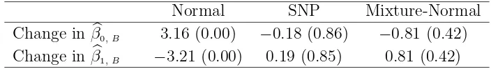
The values of T∗

1,1 and T

∗

1,2 for assessing the robustness of MLEs for β0 and β1

resulting from different modelings and the corresponding p-values are given in Ta-ble 4.4. The fact that SNP modeling gives the smallestT∗

1,1 and T

∗

1,2 in absolute value

and normal modeling yields the largest T∗

1,1 and T

∗

1,2 in absolute value is consistent

(51)

Table 4.1: Values of T∗

1,1 and T

∗

estimates when λ= 0 andλ= 3 under three ways of modeling for the simulated data used in Example 4.2. Corresponding p-values are given in the parentheses.

Normal SNP Mixture-Normal

Change in β0,b B 6.91 (0.00) 0.12 (0.90) −0.83 (0.41)

Change in β1,b B 4.99 (0.00) −0.20 (0.84) −0.32 (0.75)

1,1 and T

∗

1,2 assessing robustness of the conditional score

esti-mates and MLEs for the regression parameter under three ways of modeling when λ= 0 andλ = 3 for the simulated data used in Example 4.3. Correspondingp-values are given in the parentheses.

Normal SNP Mixture-Normal Conditional-score Change in β0,b B 5.26 (0.00) 0.65 (0.52) 0.61 (0.54) 0.12 (0.90)

Change in β1,b B 3.45 (0.00) 0.72 (0.47) 0.73 (0.47) −0.66 (0.51)

Table 4.3: Rejection rates (proportion of 100 data sets with _|T∗

1,·| > 1.96) in testing robustness of the estimates using T∗

1,1 and T

∗

1,2 for β0 and β1, respectively, when λ

varies from 0 to 3 under three ways of modeling for the simulated data. Numbers in the parentheses are estimated standard errors of the rejection rates.

Normal SNP Mixture-Normal Test the change in β0,b B 1 (0) 0.08 (0.03) 0.07 (0.03)

Test the change in β1,b B 0.99 (0.01) 0.1 (0.03) 0.1 (0.03)

1,1 and T

∗

estimates when λ = 0 and λ= 3 under three ways of modeling for the Framingham data. Correspondingp-values are given in the parentheses.

Normal SNP Mixture-Normal

Change in β0,b B 3.16 (0.00) −0.18 (0.86) −0.81 (0.42)

(52)

0.0 0.2 0.4 0.6 0.8 1.0

−0.07

−0.05

−0.03

−0.01

λ

bβ

(

.

)

0

−

bβ

(

m

)

0

(a)

0.0 0.2 0.4 0.6 0.8 1.0

−0.12

−0.08

−0.04

0.00

λ

bβ

(

.

)

1

−

bβ

(

m

)

1

(b)

Figure 4.1: Deviations from the MLEs resulting from the mixture-normal modeling when modeling X as normal and SNP, Example 4.2; (a) corresponds to βb0,B; (b)

corresponds to βb1,B. The correspondence of the line types and ways of modeling is

(53)

0.0 0.5 1.0 1.5 2.0 2.5 3.0

−0.02

0.00

0.02

0.04

λ

bβ0

(a)

0.0 0.5 1.0 1.5 2.0 2.5 3.0

0.85

0.90

0.95

1.00

λ

bβ1

(b)

Figure 4.2: MLEs under the three assumed models for X and conditional score es-timates versus λ, Example 4.3; (a) corresponds to βb0,B and βb0,∗; (b) corresponds to

b

β1,B and βb1,∗. True values of β0 and β1 are marked by the dotted reference lines.

(54)

(a) (b)

λ λ

bβ0,B bβ1,B

0

0 1 2 3 1 2 3

−

3

·

5

−

3

·

2

−

2

·

9

1

·

2

1

·

4

1

·

6

Figure 4.3: θb(Bn) (solid line),θb

(s)

B (dashed line), andθb

(m)

(55)

Chapter 5 Latent-Model Robustness in Joint

Models

5.1 Expected Robustness

We now consider joint models that have a linear mixed effect model for the longi-tudinal process, where the random effect is a latent variable. Insensitivity of inference onθ to the assumed random-effect model has been reported in the literature. Hsieh et al. (2006) gave a heuristic explanation for this insensitivity “when reasonably large numbers of longitudinal measurements are available per subject” using a Laplace ap-proximation technique. In this section, we prove more explicitly that the insensitivity to the assumed random-effect model is expected when the subject-specific information on the longitudinal process is sufficiently large.