Hydrol. Earth Syst. Sci., 17, 721–733, 2013 www.hydrol-earth-syst-sci.net/17/721/2013/ doi:10.5194/hess-17-721-2013
© Author(s) 2013. CC Attribution 3.0 License.
EGU Journal Logos (RGB)
Advances in
Geosciences
Open Access
Natural Hazards
and Earth System
Sciences
Open AccessAnnales
Geophysicae
Open AccessNonlinear Processes
in Geophysics
Open AccessAtmospheric
Chemistry
and Physics
Open AccessAtmospheric
Chemistry
and Physics
Open Access DiscussionsAtmospheric
Measurement
Techniques
Open AccessAtmospheric
Measurement
Techniques
Open Access DiscussionsBiogeosciences
Open Access Open Access
Biogeosciences
DiscussionsClimate
of the Past
Open Access Open Access
Climate
of the Past
Discussions
Earth System
Dynamics
Open Access Open Access
Earth System
Dynamics
DiscussionsGeoscientific
Instrumentation
Methods and
Data Systems
Open Access
Geoscientific
Instrumentation
Methods and
Data Systems
Open Access DiscussionsGeoscientific
Model Development
Open Access Open Access
Geoscientific
Model Development
DiscussionsHydrology and
Earth System
Sciences
Open AccessHydrology and
Earth System
Sciences
Open Access DiscussionsOcean Science
Open Access Open Access
Ocean Science
DiscussionsSolid Earth
Open Access Open Access
Solid Earth
Discussions
The Cryosphere
Open Access Open Access
The Cryosphere
DiscussionsNatural Hazards
and Earth System
Sciences
Open Access
Discussions
Role of climate forecasts and initial conditions in developing
streamflow and soil moisture forecasts in a rainfall–runoff regime
T. Sinha and A. Sankarasubramanian
Department of Civil, Construction and Environmental Engineering, North Carolina State University, Raleigh, NC, USA
Correspondence to: T. Sinha ([email protected])
Received: 21 March 2012 – Published in Hydrol. Earth Syst. Sci. Discuss.: 19 April 2012 Revised: 10 January 2013 – Accepted: 26 January 2013 – Published: 20 February 2013
Abstract. Skillful seasonal streamflow forecasts obtained
from climate and land surface conditions could significantly improve water and energy management. Since climate fore-casts are updated on a monthly basis, we evaluate the po-tential in developing operational monthly streamflow fore-casts on a continuous basis throughout the year. Further, basins in the rainfall–runoff regime critically depend on the forecasted precipitation in the upcoming months as opposed to snowmelt regimes where initial hydrological conditions (IHC) play a critical role. The goal of this study is to quan-tify the role of updated monthly precipitation forecasts and IHC in forecasting 6-month lead monthly streamflow and soil moisture for a rainfall–runoff mechanism dominated basin – Apalachicola River at Chattahoochee, FL. The Vari-able Infiltration Capacity (VIC) land surface model is imple-mented with two forcings: (a) updated monthly precipitation forecasts from ECHAM4.5 Atmospheric General Circulation Model (AGCM) forced with sea surface temperature fore-casts and (b) daily climatological ensembles. The difference in skill between the above two quantifies the improvements that could be attainable using the AGCM forecasts. Monthly retrospective streamflow forecasts are developed from 1981 to 2010 and streamflow forecasts estimated from the VIC model are also compared with those predicted by using the principal component regression (PCR) model. The mean square error (MSE) in predicting monthly streamflows, using the VIC model, are compared with the MSE of streamflow climatology under ENSO (El Ni˜no Southern Oscilation) con-ditions as well as under normal years. Results indicate that VIC forecasts obtained using ECHAM4.5 are significantly better than VIC forecasts obtained using climatological en-sembles and PCR models over 2–6 month lead time during winter and spring seasons in capturing streamflow variability
and reduced mean square errors. However, at 1-month lead time, streamflow utilizing the climatological forcing scheme outperformed ECHAM4.5 based streamflow forecasts during winter and spring, indicating a dominant role of IHCs up to a 1-month lead time. During ENSO years, streamflow fore-casts exhibit better skill even up to a six-month lead time. Comparisons of the seasonal soil moisture forecasts, devel-oped using ECHAM4.5 forcings, with seasonal streamflows also show significant skill, up to a 6-month lead time, in the four seasons.
1 Introduction
Skillful seasonal forecasts of streamflow and soil moisture are essential for water management as well as to support agricultural operations. Previous studies have shown that the application of seasonal streamflow forecasts, obtained from climate and land surface conditions, could significantly im-prove water and energy management (Yao and Georgakskos, 2001; Voisin et al., 2006; Sankarasubramanian et al., 2010; Hamlet et al., 2002). Seasonal streamflow forecasts derive their skill from slowly evolving climatic conditions, partic-ularly the Sea Surface Temperature (SST) as well as initial hydrologic conditions (IHC) such as soil moisture and snow cover (Mahanama and Koster, 2003; Maurer et al., 2004; Wood and Lettenmaier, 2008).
Oscillation (ENSO) indices, and IHC (including soil ture and snow), and reported that the role of soil mois-ture dominated forecasting skill for lead times of up to 1.5 months. Shukla and Lettenmaier (2011) quantified the role of IHC as well as observed and climatological forcings (CF) in predicting the runoff and soil moisture over the continen-tal US and found that climate forcings dominate IHC over the northeastern and southeastern US.
Streamflow forecasting skill significantly varies across rainfall–runoff and snowmelt-driven regimes. Maurer et al. (2004) reported that snow, in its dry state, played a cru-cial role in streamflow predictability of up to 4.5-month lead time in the western US. Koster et al. (2010) concluded that in snow dominated regions, the snow water equivalent (SWE) generally contributed to overall streamflow predictability; with the role of early-season soil moisture in improving streamflow prediction being relatively small. Initialization of snow also had a greater impact on the overall skill during the spring-melt season in the Northwest US, while the contribu-tion of soil moisture is particularly high in the Southeast (up to 5 or 6 months) during fall and winter (Mahanama et al., 2012). Mahanama et al. (2012) primarily employed climatol-ogy as forcings with updated initial conditions, using differ-ent LSMs (land surface model) to develop seasonal stream-flow forecasts. In the present study, the main focus is to utilize updated monthly precipitation forecasts from GCMs (global circulation model), forced with forecasted SSTs, to develop monthly streamflow forecasts and also to evaluate their skill against climatological forcings.
Most studies that developed streamflow forecasts based on land surface models have used observed or climatologi-cal forcings (e.g., Hamlet et al., 2002; Maurer and Letten-maier, 2003; Mahanama et al., 2012), while only fewer stud-ies have employed retrospective climate forecasts (Luo and Wood, 2008; Luo et al., 2007; Yuan et al., 2011). Wood et al. (2002) found that IHC played a more critical role than climate forecasts (CF) in predicting streamflow during the summer of 2000, whereas both IHC and CF were impor-tant in predicting winter streamflow during 1997–1998 El Ni˜no conditions over the southeastern US. Luo et al. (2007) used bias-corrected climate forecasts from multiple models, to predict streamflow in the Ohio River basin, and found that climate forecasts contributed more than IHC uncertainties at long-lead times, of more than one month, in the prediction of the summer flows. Li et al. (2009) pointed out that initial conditions have a dominant effect on forecasting skill over a short-term lead time (up to 1 month), while climate forcings control forecasting skill at longer lead times based on two initializations at the beginning of January and July. However, all the above studies that utilized retrospective climate fore-casts, for assessing the streamflow forecasting skill, have pri-marily focused on evaluating the skill in two critical seasons – summer and winter.
The primary intent of this study, is to quantify the role of updated monthly precipitation forecasts and initial
hydrologic conditions in the forecasting of a 6-month lead monthly streamflow for a river basin dominated by the rainfall–runoff mechanism. Given that monthly climate fore-casts are issued and updated on a regular basis (Barnston et al., 2003; Goddard et al., 2003), it is imperative to evalu-ate the potential in developing monthly streamflow forecasts on a continuous basis throughout the year, so that the de-veloped forecasts can be employed for water resources plan-ning and management. Furthermore, basins in the rainfall– runoff regime critically depend on the forecasted precip-itation in the upcoming months, as opposed to snowmelt regimes where IHC play a critical role (Mahanama et al., 2012). For this purpose, we utilize a long period of the ret-rospective monthly precipitation forecasts available (1957–to date) from the ECHAM4.5 general circulation model (GCM) (Li and Goddard, 2005). The six-month ahead precipita-tion forecasts were updated every month based on the up-dated SST forecasts developed using the constructed ana-logue method (van den Dool, 1994). Using this long time se-ries of monthly updated six-month ahead precipitation fore-casts, we perform a set of experiments to address the follow-ing research questions related to developfollow-ing monthly updated streamflow and soil moisture forecasts in a rainfall–runoff regime:
1. How does the skill in predicting observed monthly streamflow vary over different seasons and lead time? 2. How does the skill in predicting monthly streamflow
and soil moisture forecasts vary during El Ni˜no South-ern Oscillation (ENSO) conditions to normal condi-tions?
3. What contributes to the variability in the skill in devel-oping streamflow and soil moisture forecasts?
This study systematically addresses the above questions by utilizing monthly updated climate forecasts from ECHAM4.5 GCM forced with constructed analogue SST forecasts.
The manuscript is structured as follows: Sect. 2 details the study area and retrospective climate forecasts used in the study. Section 3 provides experimental details on developing monthly updated streamflow forecasts, while the results and analyses are summarized in Sect. 4. Finally, Sect. 5 presents the summary and findings from the study.
2 Study area and data
2.1 Study area
Fig. 1. Location of the Apalachicola River at Chattahoochee, FL, (a) and observed (Obs) and VIC model simulated (Sim) streamflow seasonality (b) for the VIC model evaluation period of 1981–2010 at USGS gauging station 02358000. Stars indicate location of 7 se-lected ECHAM4.5 grids. Figure 1b also shows the Nash–Sutcliff efficiency (NSE) and %bias over the entire evaluation period.
where precipitation is pretty uniform resulting in signifi-cant runoff throughout the year. Thus, developing streamflow forecasts, on a continuous basis throughout the year, is crit-ical for the region from an operational perspective as well as for management during critical seasons. For this study, we consider the entire Apalachicola River at Chattahoochee Basin, over the period 1981–2010, for the development of monthly-updated streamflow forecasts. The average annual precipitation in the basin is about 1280 mm, with no season-ality in precipitation, and the mean monthly runoff peaks in March with the lowest monthly flows occurring during the fall (Fig. 1b).
2.2 Observed meteorological and streamflow data
The daily meteorological forcing data for precipitation, max-imum and minmax-imum air temperatures, and wind speed from
1957 to 2010 were obtained from Maurer et al. (2002) at 1/8◦spatial scale (∼14 km by 12 km). The monthly observed streamflow data from 1957 to 2010 was obtained from the US Geological Survey (USGS) at Apalachicola River at Chatta-hoochee (site #02358000). This site is minimally affected by anthropogenic interventions, such as reservoir operations as it is included in the Hydro-Climatic Data Network (HCDN) database (Slack et al., 1993), and ultimately the extended USGS streamflow data were used.
2.3 ECHAM4.5 precipitation forecasts
6-month lead ECHAM4.5 monthly precipitation forecasts (Jan 81 – Dec 2010)
Spatial (CCA) downscaling of 6-month lead monthly precipitation forecasts (Jan 81 – Dec 2010)
6-month lead monthly streamflow forecasts (Jan 81 – Dec 2010)
Skill evaluation of 6-month lead monthly streamflow forecasts using observed flows Daily PRCP at 1/8o(Jan 81 – Dec 2010)
Calibrated VIC model
Routing model Update IHC’s prior to forecasting
month using 1/8o daily observed PRCP, TMAX, TMIN, and WIND
data (Jan 81 – Dec 2010)
Temporal (K-NN) disaggregation (Prairie et al., 2007) a. VICfcst
6-month lead ECHAM4.5 monthly precipitation forecasts (Jan 81 – Dec 2010)
Observed streamflow time series for 1 month prior to forecasting period Calibration: Moving window of previous 24
years on monthly flows
If lead (i) = 1?
PCR
Monthly streamflow forecasts for lead (i) = 1 – 6 months over Jan 81 – Dec 2010
If lead > 1? Update streamflow for 1 month prior
to forecasting month from previous step’s PCR output
Skill evaluation of 1 – 6 months lead forecasts using observed flows c. PCR( , fcst)
b. VICclim Update IHC’s (Jan 81 – Dec 2010) +
Daily 1/8 gridded PRCP
ensemble (Jan 57 – Dec 80) Calibrated VIC model streamflowRouted
Qtˆ1
Fig. 2. Experimental design to develop monthly updated 6-month ahead 6-monthly streamflow: (a) VICfcst, (b) VICclim, and
(c) PCR(Qˆt−1, fcst). CCA refers to Canonical Correlation
Analy-sis and K-NN represents Kernel-Nearest Neighbor approach. PRCP refers to precipitation, TMAX to maximum air temperature, TMIN to minimum air temperature, and WIND to wind speed.
3 Retrospective streamflow forecasts development
Figure 2 illustrates the experimental setup, for streamflow forecasts development, using the VIC model and the statisti-cal model.
3.1 Variable Infiltration Capacity (VIC) model
The VIC model (Liang et., 1994, 1996; Cherkauer and Let-tenmaier, 2003) is a semi-distributed macroscale land surface model that estimates water and energy balance. Streamflow is computed at the basin outlet using a stand-alone routing model (Lohman et al., 1998a, b). The details of the VIC model are described in Liang et al. (1994, 1996). The soil and vegetation input parameters are described in Sinha et al. (2010). The daily meteorological forcings are described in Maurer et al. (2002).
Table 1. Rank correlations between monthly time series of average precipitation from selected 7 ECHAM 4.5 grids for 1–6 month lead times and spatially averaged (monthly) observed precipitation over the study area during the period from 1957 to 1980.
Lead Time (months) Rank Correlation
1 0.32
2 0.32
3 0.31
4 0.34
5 0.33
6 0.31
3.1.1 VIC model calibration and evaluation
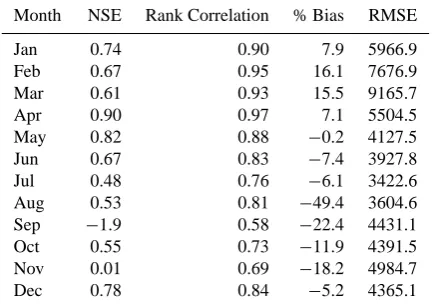
The VIC model was first calibrated for the Apalachicola River at Chattahoochee (site # 02358000), at a monthly time step from 1957 to 1980 (Table 2), using observed stream-flow obtained from the USGS. The standard VIC soil param-eters that control infiltration, runoff and subsurface flow were manually calibrated to match overall hydrograph shape and volume of observed monthly streamflow. Finally, the model was validated from 1981 to 2010 (Fig. 1b) and the overall Nash–Sutcliff efficiency (NSE) during this period was 0.81. The monthly NSE was also high for most of the months, ex-cept during the low flow months of September and Novem-ber, where it was relatively low (Table 2).
3.1.2 Temporal disaggregation
Daily time series of precipitation were derived from monthly time series using the temporal disaggregation technique de-scribed in Prairie et al. (2007). The temporal disaggregation involved classifying monthly time series into daily time se-ries by identifying similar monthly conditions in the histor-ical record based on the Kernel-nearest neighbor (K-NN) approach. A brief description is provided here for clarity. Typically, the K-NN approach resamples monthly data from daily historic data, generating values that were observed. In this study, the K-NN approach was implemented (Prairie et al., 2007), where Kernel nearest neighbors were obtained by computing the distance between predicted time series and the historic series for the period 1957–1980. The observed daily values from the “K” neighbors were resampled based on the Lall and Sharma kernel (Lall and Sharma, 1996). The number of neighbors for each month was chosen based on leave-five-out cross-validation for the training period 1957– 1980. For further details of the K-NN approach, see Prairie et al. (2007).
3.1.3 Errors due to temporal disaggregation of monthly observed precipitation
Table 2. VIC model calibration summary for the period 1957–1980. NSE represents Nash–Sutcliffe Efficiency.
Month NSE Rank Correlation % Bias RMSE
Jan 0.74 0.90 7.9 5966.9
Feb 0.67 0.95 16.1 7676.9
Mar 0.61 0.93 15.5 9165.7
Apr 0.90 0.97 7.1 5504.5
May 0.82 0.88 −0.2 4127.5
Jun 0.67 0.83 −7.4 3927.8
Jul 0.48 0.76 −6.1 3422.6
Aug 0.53 0.81 −49.4 3604.6
Sep −1.9 0.58 −22.4 4431.1
Oct 0.55 0.73 −11.9 4391.5
Nov 0.01 0.69 −18.2 4984.7
Dec 0.78 0.84 −5.2 4365.1
al. (2002) was aggregated to the monthly scale and then dis-aggregated to the daily time step using the K-NN approach. Errors due to temporal disaggregation were estimated on a monthly basis by computing the Relative Root Mean Square Error (R-RMSE) between observed daily precipitation (Mau-rer et al., 2002) and the disaggregated daily time series for the 1981–2010 period. For each day, average precipitation was estimated over the 30-yr period using daily time series of observed precipitation and disaggregated precipitation for all the 251 1/8◦grids covering the entire study area. Finally, the monthly R-RMSEs, relative to its monthly climatology, were estimated for all the 251 grids using Eq. (1):
R-RMSEt = r
n−1Pn t=1
Pt− ˆPt 2
Pt
, (1)
wheret is time in days, n is number of days in a month, Pt is observed average daily precipitation, Pˆt= temporally disaggregated average daily precipitation, andPt is the ob-served average daily precipitation (climatology) for a given month. Figure 3a indicates that relative errors, due to tempo-ral disaggregation, are higher in fall months (September to November) while errors are lower during winter and spring months. This is partly due to the limited skill in predicting the fall precipitation as well as to the increased error in the disaggregation model during these months.
3.1.4 Spatial downscaling
For each month, precipitation forecasts from 7 ECHAM4.5 grids (∼2.8◦by 2.8◦), over the Apalachicola River basin at Chattahoochee, were used to obtain monthly precipitation time series at 1/8◦ spatial resolution. Given that the fore-casts from these grid points as well as the observed pre-cipitation over 1/8◦resolution are correlated, we employed Canonical Correlation Analysis (CCA) such that the low-dimensional components of predictors and predictands were
used to develop regression models for spatial downscaling (Tippet et al., 2003; Oh and Sankarasubramanian, 2011). CCA maximizes inter-relationships between two data sets, in contrast to Principal Component Analysis (PCA) where vari-ability is maximized within a single data set (Wilks, 1995). The spatial downscaling is performed using the observed gridded data from Maurer et al. (2002) as reference. For each month, the following steps were followed to spatially down-scale precipitation forecasts:
1. Monthly anomalies (Z), for each of the 251 1/8◦grids covering the entire study area, were estimated by sub-tracting the basin’s monthly spatial average precipita-tion from the period 1957 to 1980 (pre-forecast period) from each grid’s monthly precipitation.
2. First, six principal components (e.g. YT=Y1, Y2, ...,
Y6, dimension =n×6, where n=54 yr and T denotes
transpose), which explained more than 95 % variabil-ity in precipitation anomalies of the 251 grids, were re-tained from 1957 to 2010 to reduce the dimensionality and were used as the predictands.
3. Similar to step (2), six principal components were re-tained from the anomalies of ECHAM4.5 monthly pre-cipitation forecasts that served as predictors (e.g.XT= X1,X2, ...,X6, dimension = 54×6). The
dimensional-ity of predictors was reduced from 7 to 6 components to keep it consistent with the dimensions of predictands. Retaining 7 original components versus 6 components after PCA had minimal (statistically insignificant) effect on VIC simulated monthly streamflow.
4. A CCA model was developed using a split sampling approach, where monthly data from 1957 to 1980 was used for training, while monthly precipitation from 1981 to 2010 was predicted using the CCA model. The CCA identified a linear combination of 6 predictors, X∗=aTX, which maximized linear combination of 6 predictandsY∗=bTY. The vectorsaandbwere chosen such that
aTP
XY
b
s
aTP
XX
a
bTP
Y Y
b
was maximized where P
denotes the variance–covariance matrix between the two variables (see details in Wilks, 1995).
5. The CCA estimated standardized anomalies were trans-ferred back to the original standardized anomaly space (Z) by
ZT=E·UT,
Fig. 3. Box plots of relative root mean square error for 251 1/8◦ grid cells due to: (a) temporal disaggregation of monthly observed precipitation to daily scale, and (b) spatial downscaling of 1-month lead ECHAM4.5 monthly precipitation forecasts.
6. Finally, the observed monthly spatial mean was added back to the product of standardized anomalies and monthly standard deviation to obtain the monthly time series from 1981 to 2010 for each of the 251 1/8◦grids. For less than 2 % of the cases among all the 251 grids, the spatially downscaled monthly precipitation was less than or equal to zero. In those months, a historical min-imum monthly precipitation (for the period 1957–1980) of 5 mm was assigned.
3.1.5 Errors due to spatial downscaling of monthly precipitation forecasts
Errors in spatial downscaling of 1-month lead ECHAM4.5 monthly precipitation forecasts to 251 grids at 1/8◦ spatial scale were evaluated by estimating R-RMSE using equa-tion 1, but on a monthly time step. Figure 3b suggests that the median R-RMSE at 1-month lead time is higher during fall months specifically during September through Novem-ber, which is similar to errors due to temporal disaggrega-tion. This implies that, the accuracy of the spatially down-scaled monthly precipitation forecasts in predicting the ob-served precipitation is relatively lower over the 251 1/8◦grid cells during the fall months. The relative errors are lower dur-ing sprdur-ing and summer months (Fig. 3b).
Since the statistical downscaling scheme preserves long-term mean monthly precipitation, changes in mean monthly ECHAM4.5 precipitation forecasts are statistically insignif-icant over different lead times. Finally, the daily time se-ries of precipitation were derived from spatially downscaled monthly ECHAM4.5 forecasts for 1–6 months lead time (ob-tained from CCA) using the temporal K-NN disaggregation technique, described above in Sect. 3.1, to implement a land surface model.
3.1.6 Land surface model implementation
The implementation of the VIC model was performed in the following ways (Fig. 2): (i) the VIC model was driven using observed meteorological forcings data from 1975 to 2010 in order to estimate IHCs prior to each month of fore-casting period (1981–2010) (e.g., to forecast streamflow in January 1981, IHCs at the end of December 1980 were up-dated to force the VIC model); and (ii) the statistically down-scaled and temporally disaggregated monthly precipitation forecasts from January 1981–December 2010 with lead times of 1 to 6 months were used to drive the VIC model with updated IHCs estimated from (i). Since the primary objec-tive of this study is to analyze the role of initial soil mois-ture and precipitation forecasts, other input variables such as maximum and minimum air temperatures and wind speed were used from the observed 1/8◦ meteorological forcings during the forecasting period. To compare both variabil-ity and mean errors of streamflow forecasts developed us-ing ECHAM4.5 precipitation forecasts, we also considered the Ensemble Streamflow Prediction (ESP) approach (Day, 1985; Franz et al., 2003). For developing streamflow fore-casts using ESP, we updated initial conditions every month and forced the VIC model with the climatological ensem-ble, which was developed by drawing equally likely daily ob-served precipitation over the period 1957 to 1980. For both these schemes, ECHAM4.5 forecasts and climatology, pre-dicted streamflow was routed at the basin outlet for each monthly run from the VIC model. The routed streamflow at the basin outlet were bias corrected on monthly basis based on the VIC model calibration statistics (Table 2). Percent-age bias correction on the mean monthly simulated flow for the calibration period (1957 to 1980) was estimated and was applied on the mean flow simulated for the evaluation pe-riod (1981 to 2010) for each month. Thus, for each year, the streamflow ensemble developed using the climatologi-cal ensemble was averaged to evaluate the performance mea-sures (discussed in Sect. 4). Thus, the final product from the VIC model was a bias-corrected six-month ahead monthly streamflow forecast, from January 1981 to December 2010, obtained using precipitation forecasts (VICfcst)as well as the
climatological ensembles (VICclim).
3.2 Principal Component Model – implementation
streamflow (Landman and Goddard, 2002; Sankarasubrama-nian et al., 2008). The monthly time series from 1957 to 1980 were used as the training period, with predictions be-ing made from 1981 to 2010. For predictbe-ing streamflow at a 1-month lead time, observed streamflow from the previ-ous month was used with ECHAM4.5 precipitation forecasts to predict the current month’s streamflow. For subsequent lead times (2–6 months), PCR predicted streamflow for the previous month (Qˆt−1) and precipitation forecasts (fcst) for
the corresponding month were used as predictors. Thus, for each month, six PCR models were developed under each lead time scheme using the climate predictability tool avail-able from IRI (http://portal.iri.columbia.edu/portal/server.pt? open=512\&objID=697\&PageID=7264\&mode=2). Skill obtained from the PCR model is compared with the skill ob-tained for each month using VICfcstand VICclimover the
pe-riod 1981–2010.
3.3 Forecast skill scores
The performance of VIC model and the PCR model in pre-dicting monthly/seasonal streamflow was evaluated using Spearman rank correlation and Mean Square Skill Score (MSSS). Spearman rank correlation measures the monotonic correspondence between the forecasted streamflow and the observed streamflow, and is referred to as correlation in the subsequent sections. The correlation was tested for its sta-tistical significance by checking whether the estimated cor-relation is greater than 1.96/√(n−3), wherendenotes the number of observation and forecasts pairs. MSSS indicates forecast accuracy by comparing the mean square error of the forecasts with respect to the mean square error of cli-matology (Wilks, 1995). MSSS was also estimated for each month/season using
MSSS=
1− [(Mean Square Errorforecast)/(Mean Square Errorclimatology)],(2)
where Mean Square Error (MSE)forecast is the average
squared difference between the forecast and observations pairs, and MSEclimatology is the averaged squared
differ-ence between the observations and the climatological stream-flow. The climatological estimates of streamflow are obtained by averaging the observed streamflow over 1957–1980. If MSSS is greater than zero, it indicates forecasts have better skill than climatology. Two forecasts from the VIC (VICfcst
and VICclim) model are compared with the PCR model
at monthly and seasonal time scales using correlation and MSSS. Both VICfcstand PCR have skills from IHCs and
pre-cipitation forecasts, while VICclimhas IHCs but no climate
forecast skill. VICfcst and PCR are compared by
consider-ing observed flows as reference streamflow while VICfcstand
VICclim are compared by considering VIC model simulated
flows as reference (as indicated by the subscript sim) when forced with observed meteorological forcings. Improvements in MSSS of VICfcstsimover VICclimsimquantify the fractional
reduction in mean squared error (MSE) from predicting the VIC simulated flows under observed forcings by utilizing the ECHAM4.5 precipitation forecasts. Similarly, a positive MSSS of VICclimsim quantifies the fractional reduction in MSE that could be obtained using IHCs over the observed streamflow climatology.
Since ENSO is one of the dominant climatic mode that influences the winter hydroclimatology of the south-eastern US (Ropelewski and Halpert, 1987; Devineni and Sankarasubramanian, 2010), we evaluate the skill of streamflow forecasts during ENSO conditions. Typically, El Ni˜no oscillations lead to warm and wet conditions in the southeastern US, while La Ni˜na results in cool and dry conditions. For this purpose, we consider the Ni˜no3.4 index, which was obtained from the National Climate Prediction Center (http://www.cpc.ncep.noaa.gov/ products/analysis monitoring/ensostuff/ensoyears.shtml). The Ni˜no3.4 index denotes the average SST anomalies, over 5◦N to 5◦S and 120◦to 170◦W in the tropical Pacific, with positive (negative) anomalous conditions denoting El Ni˜no (La Ni˜na). El Ni˜no (La Ni˜na) conditions were identified for each forecasting month if the past 3-month average of the Ni˜no3.4 index was above the threshold of >0.5◦C (<−0.5◦C).
4 Results and analysis
In this section, we present the rank correlation and MSSS of monthly streamflow forecasts developed using the VIC model for the period 1981–2010 as well as over the ENSO years. We also compare the correlation and MSSS with the forecasts developed using climatological forcings as well as with the forecasts developed using PCR. Following that, we present correlations between the VIC model forecasted total soil moisture and observed streamflow at multiple locations along with the spatial variability in the forecasted soil mois-ture during La Ni˜na years.
4.1 Performance of six-month ahead monthly streamflow forecasts
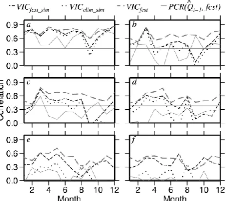
Fig. 4. Spearman rank correlations between estimated streamflow and observed streamflow at lead times 1 (a) to 6 (f) months. The horizontal gray line (at 0.38) indicates statistical significance cor-relation at 95 % confidence interval. VICfcstand VICclimrepresent
VIC model estimations when forced with ECHAM4.5 monthly pre-cipitation forecast and daily climatology ensembles, respectively. PCR(Qˆt−1, fcst) represents Principal Component Regression based
on PCR with updated initial conditions (updated previous month’s streamflow for subsequent lead times). Sim indicates VIC simulated flow as reference streamflow.
in predicting the variability in the observed streamflow over the entire year. The only exception is in September, during which the VIC model forced with climatological forcings (VICclimsim)did not result in forecasts that are statistically significant when using the VIC simulated flows as reference streamflow. Comparing the estimated rank correlation across the different forecasting schemes, we infer that VIC model based forecasting schemes perform better than PCR forecasts in almost all months, with the exceptions being February and October. The performance of VICfcstsim (ECHAM4.5) and VICclimsim is almost similar in all months except dur-ing fall months when usdur-ing VIC simulated flows as refer-ence. VICfcstoutperformed other schemes in capturing
over-all variability in observed flows.
Though the estimated correlation at 1-month lead time for VICfcstsim and VICclimsim is similar (Fig. 4a), VICclimsim per-forms better than VICfcstsim developed using ECHAM4.5 in winter and spring (Fig. 5a) based on MSSS. This indicates that the streamflow forecasts estimated using climatological forcings result in reduced mean squared error (MSE) in pre-diction as compared to the MSE of VIC forecasts obtained with ECHAM4.5 forcings during winter and spring. This in-dicates that the role of IHCs is more important than climate forecasts skills during winter and spring at 1-month lead time since VICclimsimhas only updated IHCs, while VICfcstsim
Fig. 5. Mean Square Skill Score comparison of estimated stream-flow at lead times 1 (a) to 6 (f) months.
has both updated IHCs and climate forecast skill. Given that MSSS is computed in relation to the MSE of streamflow cli-matology, MSSS basically quantifies the percentage reduc-tion in MSE of climatology resulting from the forecasting scheme. Thus, except during summer, streamflow forecasts developed from the VIC model with ECHAM4.5 forcings provide better streamflow predictions than the reference fore-cast – the streamflow climatology. In comparison to the VIC-model based forecasting schemes, the MSSS of the PCR model is generally inferior in most of the months, with the exceptions being February and October. This implies that PCR model captures only variability by exhibiting significant correlations, but the mean square errors in predicting the ob-served streamflow are relatively higher than the errors of the VIC model.
For lead times of 2 to 4 months (Figs. 4b–d and 5b–d), the PCR model performed poorly, indicating almost no skill in predicting the observed streamflow beyond 1 month. The computed correlation for the PCR model is statistically sig-nificant only in fewer months. However, VICfcstcaptures the
variability in the streamflow, exhibiting significant correla-tions in predicting the observed streamflow in all the months. Among the performance of VIC-model simulated schemes, VICfcstsim performs better than VICclimsim in all months ex-cept September to November, where both these schemes fail to capture streamflow variability. One possible reason for the poor performance of VICfcstsimduring the fall months is due to significantly higher relative errors in spatial downscaling and temporal disaggregation (Fig. 3). Evaluating the perfor-mance on the basis of MSSS also shows that VICfcst and
and VICfcstsim showed significant correlations in capturing the interannual variability in streamflow during the winter and spring season (Fig. 4e–f), but the MSSS are only positive during spring months beyond a 4-month lead time. The pri-mary reason for improved performance in capturing stream-flow variability during spring months is due to smaller inter-annual variability in precipitation during those months. We discuss this issue in detail under Discussion (Sect. 5). The significant correlation under 5–6 months for VICfcst during
spring season primarily indicates the importance of using precipitation forecasts as a forcing, as opposed to using cli-matology as a forcing.
To recapitulate, six-month ahead streamflow forecasts is-sued using VICfcst, VICfcstsimand VICclimsimhave better cor-relations and MSSS than that of the PCR model in almost all months. Similarly, VICfcstsim perform better than VICclimsim in winter and spring from 2 to 6 months lead time. The pri-mary reason for the poor performance of VIC based forecasts during the fall months is due to the poor skill in downscaled and disaggregated precipitation forecasts. The low MSSS of VICclimsim(lesser than zero) beyond one month (see Fig. 5), indicates that initial soil moisture conditions are useful only up to a month in reducing the MSE in predicting the refer-ence streamflow that could be obtainable using streamflow climatology. The improved performance of VICfcstsim over VICclimsimindicates the importance of precipitation forecasts in developing skillful monthly streamflow forecasts.
4.2 Source of skill for ECHAM4.5 forecasts – ENSO conditions
Given that streamflow forecasts developed using ECHAM4.5 forecasts performed better in capturing variability in almost all the seasons except the fall, we investigate the source of skill for ECHAM4.5 precipitation forecasts in relation to the ENSO conditions. For each month, the correlation and MSSS of VICfcst was compared with the corresponding skills of
VICclimand PCR during ENSO and non-ENSO years.
Figure 6 shows the correlation for the three forecasting schemes under four scenarios (VICfcstsim, VICclimsim, VICfcst and PCR, considering both simulated and observed flow as references) with observed/reference streamflow and over six different lead times based on ENSO conditions. At 1-month lead time, VICfcst, VICfcstsim, and VICclimsim forecasts are statistically significant in predicting the observed variabil-ity in flows in almost all months. The only exceptions are VICfcstsimand VICclimsim, being not significant in September. Comparing the correlations in Fig. 6 with Fig. 4, we un-derstand that the skill is almost similar for all the months except during October–December (OND) at 1-month lead time. Under OND, the ability to predict the variability in ob-served/reference flow is slightly higher under ENSO condi-tions for 1–2 month lead forecasts. This is because ENSO conditions typically peaks around OND. On the other hand, the correlation of the PCR model is statistically significant
Fig. 6. Similar to Fig. 4, but the skill evaluated only for ENSO con-ditions.
for 1-month lead time for the period July–March. For higher lead times, the PCR model’s skill in predicting the observed variability is statistically significant only in March.
At 3–6 month lead time, VIC-model based forecasts, VICfcstsimand VICfcst, show statistically significant skill only for the forecasts issued during spring (i.e., predicting the ob-served variability in spring flows). For forecasts issued in the rest of the months, VIC-model based forecasts did not show statistically significant skill in predicting the observed vari-ability. However, the performance of VICfcstin issuing a 3–4
month lead forecast is good for winter, spring and early sum-mer over the entire validation period (Fig. 4). We also ob-serve that the performance of VICfcstsim issued in the spring is better than that of VICclimsim.
Fig. 7. Same as Fig. 5, but MSSS calculated separately under ENSO conditions (VICfcstenso, VICclimenso) and normal tropical Pacific (VICfcstnorm, VICclimnorm)conditions.
square errors. This is consistent with the earlier findings, of Devineni and Sankarasubramanian (2010), indicating the skill of precipitation forecasts being significant only during ENSO occurrences.
The other candidates, VICclimenso and VICclimnorm did not show positive MSSS in most of the months, except during February. Thus, our analyses of splitting the MSSS shown in Fig. 7 clearly indicate that ECHAM4.5 precipitation-forecast based streamflow forecasts issued during the early winter and spring season perform well with reduced mean square errors under 2–6 month lead-times during ENSO conditions. Under neutral ENSO conditions, VICfcstnormexhibits good skill dur-ing early winter and sprdur-ing for forecasts issued with a lead time of up to 4 months. Based on this understanding, we ex-tend our analyses for developing 6-month ahead soil mois-ture forecasts.
4.3 Performance of monthly soil moisture forecasts
The VIC model simulated spatially averaged soil moisture in the top 90 cm soil layer over the two sub-basins are com-pared with the USGS observed streamflow: (a) Flint River at Newton, GA; and (b) Apalachicola River at Chattahoochee, FL (Fig. 1a). Flint River is primarily included to demonstrate the performance of soil moisture and streamflow forecasts in the upstream sub-basin, thereby exploring the potential to de-velop forecasts even for other outlet points within the basin. The correlations (Table 3) over different seasons indicate a strong relationship between spatially average soil moisture and observed seasonal streamflow over the two sites. As ex-pected, the correlations are relatively lower at longer lead times, except during the fall season (Table 3). The skill in
Table 3. Rank correlation between seasonal soil moisture forecasts and seasonal observed streamflow at (a) Flint River at Newton, GA; and (b) Apalachicola River at Chattahoochee, FL. Locations of these sites are shown in Fig. 1a. All correlations are statistically significant (>0.38).
Drainage Lead
Sub-basin Area (km2) (months) JFM AMJ JAS OND
(a) Flint 14 694 1 0.81 0.86 0.80 0.57 2 0.69 0.87 0.83 0.69 3 0.57 0.78 0.75 0.63 4 0.47 0.69 0.64 0.61 5 0.52 0.74 0.58 0.63 6 0.55 0.77 0.45 0.62
(b) Apalachicola 44 032 1 0.84 0.85 0.78 0.65 2 0.73 0.84 0.83 0.71 3 0.60 0.74 0.80 0.69 4 0.59 0.71 0.64 0.62 5 0.54 0.80 0.58 0.64 6 0.60 0.81 0.49 0.69
predicting soil moisture variability is highest at a 1-month lead time. Among all the seasons, spring season (April–June) exhibits the highest correlations followed by summer sea-son (July–September) for the two rivers. The correlations between the observed streamflow and soil moisture fore-casts are statistically significant for both the Apalachicola and Flint Rivers over the four seasons for lead times up to 6 months. Therefore, the results of VIC-model forecasted soil moisture are reasonably good for the entire basin up to a 6-month lead time.
4.4 Average soil moisture forecasts and anomalies
Fig. 8. VIC-model estimated average monthly soil moisture: (a) to (f) forecasted anomalies (at 1-month lead) estimated by subtracting total soil moisture during La Ni˜na years from soil moisture clima-tology for the period 1981 to 2010, which is shown in panels (g) to (l).
5 Discussion and concluding remarks
This study focuses on quantifying the utility of updated monthly precipitation forecasts and the role of initial soil moisture conditions in developing monthly streamflow fore-casts. We focused on a rainfall–runoff dominant basin – Apalachicola River at Chattahoochee, FL – located in the southeastern US. We calibrated the VIC land surface model to monthly observed streamflow for the study area and then forced the model with: (a) statistically downscaled and tem-porally disaggregated 6-month lead ECHAM4.5 precipita-tion forecasts, and (b) an ensemble of daily climatology es-timated for the period 1957–1980. Under both cases (a) and
(b), the initial soil moisture conditions were updated prior to the forecasting period. Thus, the difference in correlation and MSSS between the two forecasting schemes quantifies the improvements or potential degradation in skill that could be attributable to the precipitation forecasts obtained from the GCM. In addition, statistical models were also used to compare the correlation and MSSS over different lead times up to 6 months. This section provides discussion related to the three questions proposed in the introduction (Sect. 1).
5.1 Skill variations over various seasons and lead time
Results from Figs. 4 and 5 suggest that at one-month lead time monthly streamflow forecasts developed using precip-itation forecasts capture better variability, whereas monthly forecasts developed using climatological forcings have lower mean square errors during winter and spring. Since the cli-matological forcing scheme only has updated IHCs but no climate forecast skill, reduced mean errors in comparison to precipitation forecast schemes (with IHC’s and climate fore-cast skill) indicates a dominant role of IHCs during winter and spring at 1-month lead time. In particular, land surface modeling streamflow forecasts were relatively poorer than the statistical model during late summer (September) and early fall (October) months. The poor performance of pre-cipitation forecasts during these months is partly due to high R-RMSE due to spatial downscaling and temporal disaggre-gation in the precipitation forecasts.
At 2–6 month lead times, streamflow forecasts developed using the precipitation forecasts showed better correspon-dence (i.e., correlation) in matching the interannual variabil-ity of observed flows as well as in terms of accuracy with MSSS>0 during winter and spring. These findings are con-sistent with the findings of Shukla and Lettenmaier (2011), who indicated that soil moisture skills dominate up to a 1-month lead time while climate forcings dominate beyond a 1-month lead in the southeastern US. These results are also in agreement with Li et al. (2009) who reported that ini-tial conditions have a dominant effect on forecast skill up to 1 month while downscaled climate forecasts outperformed the ESP approach for longer lead times. However, the un-certainty over the longer lead times could be reduced by continuously updating the monthly streamflow forecasts as we progress through the season (Sankarasubramanian et al., 2008).
5.2 Role of ENSO conditions
clearly show that ECHAM4.5 precipitation forecasts based streamflow forecasts issued during the winter season perform well with reduced mean errors from 2–4 months lead time under neutral conditions and from 2–6 months lead time un-der ENSO conditions. However, MSSS of ECHAM4.5 based precipitation forecasts is lower than MSSS of climatologi-cal forcings based streamflow forecasts at 1-month lead time during winter and spring. This indicates that the role of IHCs is dominant up to 1-month under both ENSO and neutral con-ditions. Thus, this analysis provides critical information that during ENSO conditions, we not only have better MSSS in predicting the observed streamflow using precipitation fore-casts from GCMs beyond a 1-month lead time, but also gain increased lead time in predicting the observed flows.
5.3 Difference in skill variations in streamflow and soil moisture forecasts
Our previous discussion suggests that the primary source of variability in the skill on predicting streamflow arises from ENSO conditions. Given that we do not have observed soil moisture information, we compared the seasonal soil mois-ture forecasts to the observed seasonal streamflow. The VIC-model soil moisture forecasts compare reasonably well with the observed streamflow at two sites, particularly, up to a 6-month lead time. VIC-model soil moisture climatology sug-gests that April is the wettest while September is the driest month in the growing season. During La Ni˜na conditions, the drying effect is more pronounced in June and August months. The correlation between the soil moisture forecasts for the winter and spring seasons and the corresponding observed seasonal streamflow increase as the drainage area increases. On the contrary, the correlation between the soil moisture forecasts, for the summer season, and the observed stream-flow decrease as the drainage area increases. This is primarily due to the increased role of temperature during the summer season leading to enhanced evapotranspiration over a larger area, resulting in decreased correlation with streamflow.
Climate forecasts from the ECHAM4.5 GCM along with the updated initial conditions provide useful information which can be utilized in improving the management of wa-ter and energy systems. This study quantified the additional skill that could be gained using precipitation forecasts from ECHAM4.5 forecasts over the climatological forcings. This study uses precipitation forecasts from one GCM; however, combining climate information from multiple models has been shown to result in improved streamflow forecasts (Devi-neni et al., 2008). The climatological forcings were run as en-semble and the mean of the streamflow enen-semble was used to quantify the skill. On the other hand, we forced the VIC model with downscaled ensemble mean precipitation fore-casts due to the challenges in downscaling of finite size of probabilistic forecast ensembles (Wilks and Hamill, 2007; Wilks, 2009). Running the hydrological model using the downscaled and disaggregated forecasts based on each and
every ensemble member of ECHAM4.5 precipitation fore-casts is beyond the scope of this paper. We hope to address this in future research by pursuing ensemble-MOS methods as suggested by Wilks and Hamill (2007). Further, it also needs to be analyzed how spatial downscaling and tempo-ral disaggregation contribute to the limited skill during the fall season since the statistical model seems to outperform both VIC-model based forecasting schemes. Since basins in the southeastern US have no seasonality in precipitation, it is also important to understand the source of error arising from the downscaling and disaggregation scheme. We intend to address these issues as part of our continuing research on developing operational streamflow forecasts over the south-eastern US.
Acknowledgements. We are thankful to NOAA for providing
funding for this research through grant NA09OAR4310146. We also thank the reviewers for providing useful suggestions which helped to improve overall quality of the manuscript.
Edited by: A. Gelfan
References
Barnston, A. G., Mason, S. J., Goddard, L., Dewitt, D. G., and Ze-biak, S. E.: Multimodel ensembling in seasonal climate forecast-ing at IRI, B. Am. Meteorol. Soc., 84, 1783–1796, 2003. Cherkauer, K. A. and Lettenmaier, D. P.: Simulation of spatial
vari-ability in snow and frozen soil. J. Geophys. Res., 108, 8858, doi:10.1029/2003JD003575, 2003.
Day, G. N.: Extended Streamflow Forecasting Using NWSRFS, J. Water Res. Pl.-ASCE, 111, 157–170, 1985.
Devineni, N. and Sankarasubramanian, A.: Improved categorical winter precipitation forecasts through multimodel combinations of coupled GCMs, Geophys. Res. Lett., 37, L24704, 1–22, doi:10.1029/2010GL044989, 2010.
Devineni, N., Sankarasubramanian, A., and Ghosh, S.: Multi-model ensembles of streamflow forecasts: Role of predictor state in developing optimal combinations, Water Resour. Res., 44, W09404, doi:10.1029/2006WR005855, 2008.
Franz, K. J., Hartmann, H. C., Sorooshian, S., and Bales, R.: Verifi-cation of National Weather Service ensemble streamflow predic-tions for water supply forecasting in the Colorado River basin, J. Hydrometeorol., 4, 1105–1118, 2003.
Goddard, L., Barnston, A. G., and Mason, S. J.: Evaluation of the IRI’s “net assessment” seasonal climate forecasts: 1997–2001, B. Am. Meteorol. Soc., 84, 1761–1781, 2003.
Hamlet, A. F., Huppert, D., and Lettenmaier, D. P.: Economic value of long-lead streamflow forecasts for Columbia River hy-dropower, J. Water Res. Pl.-ASCE, 128, 91–101, 2002. Koster, R. D., Mahanama, S. P. P., Livneh, B., Lettenmaier, D. P.,
and Reichle, R. H.: Skill in streamflow forecasts derived from large-scale estimates of soil moisture and snow, Nat. Geosci., 3, 613–616, 2010.
Landman, W. A. and Goddard, L.: Statistical recalibration of GCM forecasts over southern Africa using model output statistics, J. Climate, 15, 2038–2055, 2002.
Li, H., Luo, L., Wood, E. F., and Schaake, J.: The role of initial conditions and forcing uncertainties in seasonal hydrologic forecasting, J. Geophys. Res., 114, D04114, doi:10.1029/2008JD010969, 2009.
Li, S. and Goddard, L.: Retrospective Forecasts with the ECHAM4.5 AGCM, IRI Technical Report, 05–02, avail-able at: http://iri.columbia.edu/outreach/publication/report/ 05-02/report05-02.pdf (last access: 7 July 2012), The Earth Institue, Columbia University, New York, 2005.
Liang, X., Lettenmaier, D. P., Wood, E. F., and Burges, S. J.: A simple hydrologically based model of land surface water and en-ergy fluxes for general circulation models, J. Geophys. Res., 99, 14415–14428, 1994.
Liang, X., Lettenmaier, D. P., and Wood, E. F.: One-dimensional statistical dynamic representation of sub-grid spatial variability of precipitation in the two layer variable infiltration capacity model, J. Geophys. Res., 101, 21403–21422, 1996.
Lohmann, D., Raschke, E., Nijssen, B., and Lettenmaier, D. P.: Re-gional scale hydrology: I. Formulation of the VIC-2L model cou-pled to a routing model, Hydrolog. Sci. J., 43, 131–142, 1998a. Lohmann, D., Raschke, E., Nijssen, B., and Lettenmaier, D. P.:
Re-gional scale hydrology: II. Application of the VIC-2L model to the Weser River, Germany, Hydrolog. Sci. J., 43, 143–158, 1998b.
Luo, L. and Wood, E. F.: Use of Bayesian Merging Techniques in a Multimodel Seasonal Hydrologic Ensemble Prediction System for the Eastern United States, J. Hydrometeorol., 9, 866–884, 2008.
Luo, L., Wood, E. F., and Pan, M.: Bayesian merging of multiple climate model forecasts for seasonal hydrological predictions, J. Geophys. Res., 112, D10102, doi:10.1029/2006JD007655, 2007. Mahanama, S. and Koster, R.: Intercomparison of soil moisture memory in two land surface models, J. Hydrometeorol., 4, 1134– 1146, 2003.
Mahanama, S., Livneh, B., Koster, R., Lettenmaier, D. P., and Re-ichle, R.: Soil moisture, snow, and seasonal streamflow fore-casts in the United States, J. Hydrometeorol., 13, 189–203, doi:10.1175/JHM-D-11-046.1, 2012.
Maurer, E. P. and Lettenmaier, D. P.: Predictability of seasonal runoff in the Mississippi River basin, J. Geophys. Res., 108, 8607, doi:10.1029/2002JD002555, 2003.
Maurer, E. P., Wood, A. W., Adam, J. C., Lettenmaier, D. P., and Nijssen, B.: A long-term hydrologically based dataset of land surface fluxes and states for the conterminous Unites States, J. Climate, 15, 3237–3251, 2002.
Maurer, E. P., Lettenmaier, D. P., and Mantua, N. J.: Variability and potential sources of predictability of North American runoff, Water Resour. Res., 40, W09306, doi:10.1029/2003WR002789, 2004.
Oh, J. and Sankarasubramanian, A.: Interannual hydroclimatic vari-ability and its influence on winter nutrients varivari-ability over the southeast United States, Hydrol. Earth Syst. Sci. Discuss., 8, 10935–10971, doi:10.5194/hessd-8-10935-2011, 2011. Prairie, J., Rajagopalan, B., Lall, U., and Fulp, T.: A
stochas-tic nonparametric technique for space-time disaggregation of streamflows, Water Resour. Res., 43, W03432, 1–10,
doi:10.1029/2005WR004721, 2007.
Ropelewski, C. F. and Halpert, M. S.: Global and Regional Scale Precipitation Patterns Associated with the El-Nino Southern Os-cillation, Mon. Weather Rev., 115, 1606–1626, 1987.
Sankarasubramanian, A., Sharma, A., Lall, U., and Espinueva, S.: Role of retrospective forecasts of GCMs forced with persisted SST anomalies in operational streamflow forecasts development, J. Hydrometeorol., 9, 212–227, 2008.
Sankarasubramanian, A., Lall, U., Devineni, N., and Espinueva, S.: The Role of Monthly Updated Climate Forecasts in Improving Intraseasonal Water Allocation, J. Appl. Meteorol. Clim., 48, 1464–1482, 2010.
Shukla, S. and Lettenmaier, D. P.: Seasonal hydrologic predic-tion in the United States: understanding the role of initial hy-drologic conditions and seasonal climate forecast skill, Hy-drol. Earth Syst. Sci., 15, 3529–3538, doi:10.5194/hess-15-3529-2011, 2011.
Sinha, T., Cherkauer, K. A., and Mishra, V.: Impacts of historic cli-mate variability on seasonal soil frost in the Midwestern United States, J. Hydrometeorol., 11, 229–252, 2010.
Slack, J. R., Lumb, A., and Landwehr, J. M.: Hydro-Climatic Data Network (HCDN) Streamflow Data Set, 1874–1988, US Geolog-ical Survey Report, USGS open-file report, 92–129, available at: http://pubs.usgs.gov/wri/wri934076/, 1993.
Tippett, M. K., Anderson, J. L., Bishop, C. H., Hamill, T. M., and Whitaker, J. S.: Ensemble square-root filters, Mon. Weather Rev., 131, 1485–1490, 2003.
van den Dool, H. M.: Searching for analogues, how long must one wait?, Tellus A, 46, 314–324, 1994.
Voisin, N., Hamlet, A. F., Graham, L. P., Pierce, D. W., Barnett, T. P., and Lettenmaier, D. P.: The role of climate forecasts in Western US power planning, J. Appl. Meteorol. Clim., 45, 653– 673, 2006.
Wilks, D. S.: Statistical Methods in the Atmospheric Science, Aca-demic Press, 467 pp., San Diego, California, 1995.
Wilks, D. S.: Extending logistic regression to provide full-probability distribution MOS forecasts, Meteor. Appl., 16, 361– 368, 2009.
Wilks, D. S. and Hamill, T. M.: Comparison of Ensemble-MOS Methods Using GFS Forecasts, Mon. Weather Rev., 135, 2379– 2390, 2007.
Wood, A. W. and Lettenmaier, D. P.: An ensemble approach for attribution of hydrologic prediction uncertainty, Geophys. Res. Lett., 35, L14401, doi:10.1029/2008GL034648, 2008.
Wood, A. W., Maurer, E. P., Kumar, A., and Lettenmaier, D. P.: Long-range experimental hydrologic forecasting for the Eastern United States, J. Geophys. Res., 107, 4429, doi:10.1029/2001JD000659, 2002.
Yao, H. and Georgakakos, A.: Assessment of Folsom Lake response to historical and potential future climate scenarios: 2. Reservoir management, J. Hydrol., 249, 176–196, 2001.