A Reconstruction based Finite Volume Method for Diffusion Equation on Unstructured Grids.

by

Abhinav Sharma

A thesis submitted to the Graduate Faculty of North Carolina State University

in partial fulfillment of the requirements for the degree of

Master of Science

Aerospace Engineering

Raleigh, North Carolina 2011

APPROVED BY:

_______________________________ ______________________________

Dr. Hong Luo Dr. Jack Edwards Committee Chair

________________________________

BIOGRAPHY

Abhinav Sharma has received his Bachelor in Technology from VIT University, India in Mechanical Engineering. Currently he is pursuing the degree of Master of Science from North Carolina State University, USA in Aerospace Engineering.

ACKNOWLEDGMENTS

TABLE OF CONTENTS

List of Tables…...…….……….……….….... vii

List of Figures ….………... ix

Chapter 1 Introduction ………... 1

1.1 Background and Motivation ……….………...………...…. 2

1.2 Scope of Thesis ……….………...… 5

1.3 Outline of Thesis ……….………. 5

Chapter 2 Governing Equations and Numerical Methods ….……….…….... 7

2.1 Problem Definition ... 7

2.2 Numerical Methods ……….………..……... 7

2.2.1 Finite Volume Formulation ………..………..…..… 7

2.2.2 Common Approaches for estimation of Gradients at Interfaces ………..….... 8

2.2.3 Reconstruction Scheme ………..…… 11

2.3 Solving System of Equations ………..………... 18

2.3.1 Generalized Minimum Residual (GMRES) ………..…………. 18

2.3.2 Implementation of GMRES ………..…………. 19

2.3.3 Preconditioner ………..……..… 20

2.3.4 Jacobian Evaluation ………..…………. 21

2.3.5 Diagonal Preconditioner ………..……….. 25

2.3.6 LU-SGS Preconditioner ……….……….…... 25

2.3.7 ILU Preconditioner ……….……….….. 26

Chapter 3 An Analysis of Existing Viscous Flux Formulae …….…..………... 28

3.1 Model Grid Topology and Formulae ……….………….………... 28

3.2 Discrete Maximum Principle ………….……….………... 29

3.3 Accuracy ……….……….……..… 30

3.4 Consistency ……….……….……..… 31

3.5 Common Approaches for estimation of gradients at Cell Interfaces …….….……... 32

3.5.1 Modified Average Gradient Method ……….... 32

3.6 Reconstruction Scheme ……….……….… 39

Chapter 4 Numerical Experiments ………...…………..……….. 43

4.1 Assessment of Condition Number ……….……….……... 43

4.2 Positivity Study ………….………..……..………. 46

4.3 Accuracy Study ………..……… 49

4.4 Accuracy Study on Distorted Meshes………..….……….. 63

4.5 Study on Heterogeneous Diffusion Tensor ………..……….. 71

4.6 Convergence Analysis ………..…...……….. 74

4.7 Comparison for Reconstruction scheme and Modified Gradient Average ……....… 76

Conclusion ……… 83

LIST OF TABLES

Table 2.1 Number of columns and groups formed after CPR algorithm …………..…….. 25 Table 4.1 Condition Numbers for gradient at cell centers for Regular Triangular Meshes..44 Table 4.2 Condition Numbers for gradient at cell center for Unstructured Meshes ………44 Table 4.3 Condition Numbers for gradients at cell centers for Anisotropic Meshes …….. 44 Table 4.4 Condition Numbers for gradient at cell interfaces for Regular Triangular

Meshes………..…45 Table 4.5 Condition Numbers for gradient at cell interfaces for Anisotropic Meshes …... 45 Table 4.6 Condition Numbers for gradient at cell interfaces for Unstructured Meshes …. 45 Table 4.7 Results for test case 1 on Regular Triangular Meshes for Accuracy Study….... 49 Table 4.8 Results for test case 1 on Unstructured Meshes for Accuracy Study…………. 50 Table 4.9 Results for test case 1 on Anisotropic Meshes for Accuracy Study …....…….. 50 Table 4.10 Comparison between Reconstruction scheme and CDG Methods ...………….. 51 Table 4.11 Comparison between Reconstruction and Recovery methods ……..………... 53 Table 4.12 Results for test case 2 on Regular Triangular Meshes for Accuracy Study….... 54 Table 4.13 Results for test case 2 on Unstructured Meshes for Accuracy Study ….…..….. 55 Table 4.14 Results for test case 2 on Anisotropic Meshes for Accuracy Study …………... 55 Table 4.15 Results for test case 3 on Regular Triangular Meshes for Accuracy Study …... 58 Table 4.16 Results for test case 3 on Unstructured Meshes for Accuracy Study ...…..….. 58 Table 4.17 Results for test case 3 on Anisotropic Meshes for Accuracy Study …………... 59 Table 4.18 Results for test case 4 on Regular Triangular Meshes for Accuracy Study ... 60 Table 4.19 Results for test case 4 on Unstructured Meshes for Accuracy Study …………. 60 Table 4.20 Results for test case 4 on Anisotropic Meshes for Accuracy Study …...…..….. 61 Table 4.21 Results for test case 1 for accuracy study on distorted meshes with Distortion

Parameter = 0.6……….……….…..65 Table 4.22 Results for test case 2 for accuracy study on distorted meshes with Distortion

Parameter = 0.6……….……….…..66 Table 4.23 Results for test case 3 for accuracy study on distorted meshes with Distortion

Table 4.24 Results for test case 3 for accuracy study on distorted meshes with Distortion Parameter = 0.6……….……….…..68 Table 4.25 Results for test case 3 for accuracy study on distorted meshes with Distortion

Parameter = 0.8……….……….…..69 Table 4.26 CPU Times and number of iterations taken by each Preconditioner ………..… 74 Table 4.27 Comparison between reconstruction scheme and modified gradient approach on

Regular Triangular meshes for test case 1 ……..………..……….…. 77 Table 4.28 Comparison between reconstruction scheme and modified gradient approach on

Unstructured meshes for test case 1 ………... 78 Table 4.29 Comparison between reconstruction scheme and modified gradient approach on

Anisotropic meshes for test case 1 ………..……….. 78 Table 4.30 Comparison between Reconstruction and Modified Average Approach over set

LIST OF FIGURES

Figure 2.1 Diamond Path Reconstruction. Simple Path.……..….……...…………...…. 11

Figure 2.2 A Typical Triangular element with neighboring cells…….…..………. 12

Figure 2.3 Two Neighboring cells considered as a union..……….……….… 15

Figure 2.4 A union of two neighboring cells..……….………. 19

Figure 3.1 A Uni-Directional Stretched Grid ……...……….……...………...… 28

Figure 3.2 Diamond Path Reconstruction Stencil ………..………. 34

Figure 3.3 Simple Averaging Procedures at Subtended Vertex ….……..………... 35

Figure 3.4 Simple Reconstruction Diamond Path ………..………. 36

Figure 3.5 Stencil for Diamond Path Reconstruction on Uni-Directional Stretched Grids………..……….. 37

Figure 3.6 1D Uni-Directional Stretched Mesh ………..…….……….... 38

Figure 4.1 Sets of Meshes used for experiments of Non Negativity …………..………. 47

Figure 4.2 Results of Non Negativity tests on sets of Meshes considered …………..… 48

Figure 4.3 Plots for comparison between reconstruction and CDG method ……..….… 52

Figure 4.4 Plots for order of Accuracy for test case 1 and test case 2 on different meshes Considered…..…...……...….……….… 56

Figure 4.5 Contour Plots for Numerical Solution and Exact Solution for test case 2 …. 57 Figure 4.6 Logarithmic Plots for order of Accuracy for test case 3 and test case 4 for Different meshes……...…...……..………... 62

Figure 4.7 Contour plots for Numerical Solution and Exact solution for test case 4... 62

Figure 4.8 Different types of Distorted Meshes considered ……..………....………….. 63

Figure 4.9 Refined Distorted Meshes with Distortion Parameter as 0.6 ………...… 64

Figure 4.10 Logarithmic Plots for test case 1 and test case 2 for Accuracy Study on Distorted Meshes………...………..………...… 67

Figure 4.11 Logarithmic Plots for test case 3 for Accuracy Study on Distorted Meshes with Different diffusion parameter……...………...… 69

Figure 4.13 Results showing Jumps across Mesh Edges in case of an anisotropic

mesh... 72 Figure 4.14 Plots of Log (Residual) and Number of Iterations ……...…..………... 74 Figure 4.15 Plots of Log (Residual) with CPU times for GMRES with different

Preconditioners ………...………..………. 75 Figure 4.16 Mesh Topologies of Symmetric Stretched and Non Symmetric Stretched

Meshes ………...……….……. 76 Figure 4.17 Comparisons between Reconstruction Scheme and Modified Average

Chapter 1

Introduction

Computational Fluid Dynamics, once a domain of researchers and scholars is fast moving to the hands of engineers and professionals who are responsible for making industrial applications of CFD possible. This rapid transformation is fuelled further with enhancement of the computing power available today. Thus many industries rely heavily on the computer simulation than experimental work. Thus CFD has established itself as a viable tool for engineering analysis and design. As more and more complex flow phenomenon are being explored for complex geometries thus even more sophisticated algorithms are developed which are not only accurate but also computationally and economically efficient. Similarly flow over complex geometries are tackled using unstructured grids instead of structured grids as unstructured grids provide more accurate representation of complex geometries in mesh form.

solved by the computer. Classical CFD has following techniques for discretization finite difference methods, finite volume methods, finite element methods, spectral methods, finite point methods and discontinuous Galerkin Methods. Out of these methods finite volume methods today form a major chunk of industrial applications of CFD.

Discretizations using finite volume methods are most sought after as they use the integral conservation form of the governing equations. Thus they are not limited by discontinuities unlike finite difference methods. Because of their approach of using a control volume they can be easily used for unstructured and arbitrary grids too. The finite volume discretization of Navier Stokes equations requires an estimation of convective and diffusive fluxes for each element. The convective fluxes have been extensively worked with. There are schemes like upwind, Van Leer Scheme etc for convective fluxes. But the diffusive fluxes have received little attention. One primary reason for it is the estimation of gradients of the flow property at the interfaces of the elements. For structured grids the interfacial gradients are estimated simply by taking an average of the cell center gradients but for unstructured grids this method is not adopted.

1.1

Background and Motivation

element used whether triangular, polygonal etc. Our scheme has been made to satisfy all these requirements [24, 36, 40]. A detailed numerical analysis is in chapter 4.

described by Lipnikov et al. These schemes were found to be violating the Monotonicity Requirement [22]. A reconstruction based discontinuous method is explained by Luo et al for Navier Stokes equations. Least squares reconstruction is used here to extrapolate a smooth solution using inter cell reconstruction method. Here the authors use discontinuous Galerkin Method which are shown to be more efficient, highly parellizable and more accurate. The methods are similar to the finite volume methods with respect to determining the solution at the interfaces of the elements [18]. An approach of using finite volume methods with diffusion problem is demonstrated by Gassner et al. Here the exact solutions of diffusive Riemann problem are used to define the finite volume numerical scheme leading to a space time formulation for convection diffusion equations but this scheme cannot use a piecewise constant values for the diffusion problems as this leads to inconsistency thus at least a piecewise linear is to be taken. The order of convergence is found to be same as the degree of piecewise solution approximated [15].

solutions were obtained using the scheme but the computational costs and times were very high compared to the lower order schemes [29]. Another work on implicit integration using GMRES is done by Michalak et.al and Luo et al. A matrix free implementation of GMRES is used and an explicit jacobian matrix is calculated for usage as a preconditioner [6, 17]. Jacobian evaluation is reported in literature as most time taking activity in solving the system. Hence CPR algorithm is used in the present work for numerical jacobian evaluation which uses consistent partition of the columns [4]. This method is very advantageous as it reduces the number of function evaluations drastically. The need for even better convergence of GMRES leads to the use of preconditioners. Incomplete factorization of the preconditioner is found to be more efficient in this case.

1.2 Scope of Thesis

1.3 Outline of Thesis

Chapter 2

Governing Equations and Numerical Methods

This chapter discusses the problem statement and the methodology adopted in the present work. The treatment of boundary conditions and the gradient calculation at boundary faces and elements are also discussed here. Finally solving the system of equations implicitly is highlighted.

2.1 Problem Definition

The problem considered in this work is the diffusion equation with Dirichlet boundary condition as follows,

−∇ . 𝐷∇ 𝑈 = 𝑓 𝑖𝑛 𝛺 (2.1) 𝑈 = 𝑔 𝑜𝑛 Г = 𝜕𝛺

where, U is the physical property for which the governing equation is to be solved, Ω is a bounded domain in 𝑅2 _{and Г represents the boundary of the domain where Dirichlet} boundary condition is applied. F is the source term, D is the diffusion tensor and g is the boundary value.

2.2 Numerical Methods

2.2.1 Finite Volume Formulation

In finite volume formulation the computational space is divided into a set of computational cells. The integral formulation of the governing equation can be expressed as follows,

− ∇ . 𝐷∇ 𝑈

𝛺𝑖

𝑑𝛺 = 𝑓𝑑𝛺

𝛺𝑖

𝛺_𝑖 is the area of the ith element. The integral of the flux term over the control volume is reduced to the surface integral over the faces or walls of control element using the Green Gauss theorem as in equation 2.3.

− 𝐷∇ 𝑈 . 𝑛 𝑑Г = 𝑓𝑑𝛺

𝛺𝑖 Г𝑖

(2.3)

where, Г𝑖 is the boundary of 𝛺𝑖 control volume and 𝑛 is the surface normal to the face. Considering the discretization of only flux term from equation 2.2 and thus dropping the ‘-‘sign for convenience, we have

∇ . 𝐷∇ 𝑈

𝛺𝑖

𝑑𝛺 = 𝐷∇ 𝑈 . 𝑛 𝑑Г

Г𝑖

= 𝐷∇ 𝑈 . 𝑛

𝑖𝑓𝑎𝑐𝑒 𝑛𝐹𝑎𝑐𝑒

𝑖𝑓𝑎𝑐𝑒 =1

2.4

𝑛𝐹𝑎𝑐𝑒, represents the number of faces of the element. Thus for carrying out the finite volume discretization of the flux terms we need to calculate the gradients at the interfaces. The estimation of the gradients at the cell interfaces has been the focus of research in the present work.

2.2.2 Common Approaches used for estimating gradients at cell interfaces

Many methods have been developed in the literature for the computation of face gradient. Two most commonly adopted methods are discussed next.

Method 1: Gradient Computation based on modified averaging

∇ 𝑈

𝑓𝑎𝑐𝑒 = 0.5 ∇ 𝑈𝐿+ ∇ 𝑈𝑅 (2.5)

∇ 𝑈

𝑓𝑎𝑐𝑒 is the averaged gradient. ∇ 𝑈𝐿 and ∇ 𝑈𝑅 are the gradients of the elements left and right of the interface but this method produces checkboard instability. The solution to this problem is by adopting a gradient in the direction of the vector connecting the cell centers i.e.

𝜕𝑈

𝜕𝑙_{𝐿𝑅 𝑓𝑎𝑐𝑒} =

𝑈_𝑅 − 𝑈_𝐿

𝑙 _𝐿𝑅 (2.6)

Finally, the average gradient is modified as

∇ 𝑈 _{𝑓𝑎𝑐𝑒} = ∇ 𝑈 𝑓𝑎𝑐𝑒 − ∇ 𝑈 𝑓𝑎𝑐𝑒 . 𝑙_𝐿𝑅 𝑙 𝐿𝑅 −𝑈𝑅 − 𝑈𝐿 𝑙 𝐿𝑅 𝑙 _𝐿𝑅 𝑙 𝐿𝑅 (2.7) 𝑙_𝐿𝑅

_{is the vector between the cell centers of right and left cells and 𝑙 𝐿𝑅 denotes the distance}

between the cell centers. Although this method is not compact as it involves neighbors of neighbors, it is grid transparent. This method maintains positivity and it is inconsistent for stretched meshes as will be shown in the analysis in chapter 3 section 3.4. A comparative study in chapter 3 between this scheme and the reconstruction scheme show that the modified average scheme is less accurate for non uniform grids.

Method 2: Gradient computation based on Gauss Divergence Theorem using Diamond Path

The value of the physical property is evaluated at the vertices using interpolation. The interpolation is supported by a set of elements that share a particular vertex. An improvement is done by more accurate way of finding the values at the vertices. In the improved scheme the reconstruction is identical but uses a linearly preserving weighting function to find the values at the vertices. The weighting makes sure that the data provided to the reconstruction procedure is obtained linearly using the centroidal data. More study on the linearity preserving scheme is done in chapter 3. In terms of weighting the value at the vertex is given as,

𝑈𝑣𝑒𝑟𝑡𝑒𝑥 =

𝜔_𝑛𝑈_𝑛

𝑁 𝑛 =1

𝜔_𝑛

𝑁 𝑛=1

(2.8)

where, N is the number of cells that share the vertex and 𝜔𝑛 = 1 for all n for a simple averaging procedure. With no linearity preserving technique, this scheme is dangerously inconsistent while for linearity preserving techniques at least local grid convergence can be achieved but consistency is not guaranteed although positivity is maintained. Thus another technique, quadratic preserving scheme is used which is consistent and more accurate but less positive.

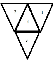
Figure 2.1 Diamond Path Reconstruction. Simple Path

2.2.3 Reconstruction Scheme

The finite volume formulation of diffusive fluxes requires estimation of gradients at the cell interfaces, which also necessitates the estimation of gradients at the cell centers. Present work concentrates on such a gradient estimation scheme namely Reconstruction Finite Volume (RFV). Least squares reconstruction forms the basis of this scheme. There are two types of reconstruction carried out in this work namely,

a) In-Cell Reconstruction b) Inter-Cell Reconstruction

a)

In-Cell Reconstruction

The gradients at the cell centers are reconstructed using the in-cell reconstruction from the underlying finite volume formulation. Calculation of the gradients at the cell centers is done using Taylor’s expansion for the neighboring cell. Consider an element I with the neighboring elements as shown in figure 2.2 namely 1, 2 and 3. We use the normalized form of the Taylor’s expansion. The normalized form gives the better conditioned matrix than non

A = Centroid 1 B = Vertex 1 C = Centroid 2 D = Vertex 2 A

B

C

normalized form, as explained in section 4.2 of chapter 4. Thus normalized form is better conditioned and reduces the stiffness of the matrix. Equation 2.9 to 2.11 represent the normalized form of Taylor’s expansion for ith

cell to the neighboring cells as shown in figure 2.2.

Figure 2.2 A typical triangular element with neighboring cells

𝑈1 = 𝑈𝑖 +

𝜕𝑈 𝜕𝑥 ∆𝑥𝑖

𝑥₁− 𝑥_𝑖 ∆𝑥𝑖

+ 𝜕𝑈 𝜕𝑦 _𝑖∆𝑦𝑖

𝑦₁− 𝑦_𝑖 ∆𝑦𝑖

(2.9)

𝑈₂ = 𝑈_𝑖 + 𝜕𝑈 𝜕𝑥 ∆𝑥𝑖

𝑥2− 𝑥𝑖

∆𝑥_𝑖 + 𝜕𝑈 𝜕𝑦 _𝑖∆𝑦𝑖

𝑦2− 𝑦𝑖

∆𝑦_𝑖 (2.10)

𝑈₃ = 𝑈_𝑖 + 𝜕𝑈 𝜕𝑥 ∆𝑥𝑖

𝑥3− 𝑥𝑖

∆𝑥_𝑖 + 𝜕𝑈 𝜕𝑦 _𝑖∆𝑦𝑖

𝑦3− 𝑦𝑖

∆𝑦_𝑖 (2.11)

where, ∆𝑥𝑖 = 0.5 𝑥𝑚𝑎𝑥 − 𝑥𝑚𝑖𝑛 𝑎𝑛𝑑 ∆𝑦𝑖 = 0.5 𝑦𝑚𝑎𝑥 − 𝑦𝑚𝑖𝑛 .

𝑥1− 𝑥𝑖

∆𝑥_𝑖

𝑦1 − 𝑦𝑖

∆𝑦_𝑖 𝑥₂− 𝑥_𝑖

∆𝑥𝑖

𝑦₂− 𝑦_𝑖 ∆𝑦𝑖

𝑥3− 𝑥𝑖

∆𝑥_𝑖

𝑦3− 𝑦𝑖

∆𝑦_𝑖 𝜕𝑈 𝜕𝑥 _𝑖∆𝑥𝑖 𝜕𝑈 𝜕𝑦 _𝑖∆𝑦𝑖 =

(𝑈₁− 𝑈_𝑖) (𝑈₂− 𝑈_𝑖) (𝑈3− 𝑈𝑖)

(2.12)

Such a system can be solved by using normal equation approach. The normalized form of coefficient matrix gives a better conditioned system. The condition number is calculated in the chapter 4 and a comparison is also made between normalized and non normalized system.

b)

Inter-Cell Reconstruction

The inter-cell reconstruction reconstructs a linear polynomial solution at each interface. In this scheme a union of two neighboring cells is considered as in figure 2.3. A linear polynomial is reconstructed as shown in equation 2.13.

𝑈𝑖𝑗 = 𝑈 + 𝑖𝑗

𝜕𝑈

𝜕𝑥 _𝑖𝑗 𝑥 − 𝑥𝑖𝑗 + 𝜕𝑈

𝜕𝑦 _𝑖𝑗 𝑦 − 𝑦𝑖𝑗 (2.13)

where, 𝑈 𝑖𝑗 is the cell averaged value in the union of two cells, (𝑥𝑖𝑗, 𝑦𝑖𝑗) are the coordinates of the centroid of the union. The averaged value of the flow parameter at the centroid of the union is given by conservation.

Similarly, the centroid of the union of two cells can be calculated using the area weighted average of coordinates of the cell centers.

𝑥_𝑖𝑗 =𝑥𝑖𝛺𝑖 + 𝑥𝑗𝛺𝑗

𝛺_𝑖 + 𝛺_𝑗 (2.16) 𝑦_𝑖𝑗 =𝑦𝑖𝛺𝑖 + 𝑦𝑗𝛺𝑗

𝛺𝑖+ 𝛺𝑗

(2.17)

(𝑥𝑖, 𝑦𝑖) are the coordinates of the center of cell I and 𝛺𝑖 is the area of the element.

At (𝑥 = 𝑥𝑖 𝑎𝑛𝑑 𝑦 = 𝑦𝑖) the function value as given by equation 2.13 is equal to the function value at the center of cell I thus 𝑈_𝑖𝑗 = 𝑈_𝑖. Thus for cells 𝑖 𝑎𝑛𝑑 𝑗, linear reconstructed polynomials in normalized form can be written as in equation 2.18 and 2.19.

𝑈𝑖 = 𝑈 + 𝑖𝑗 𝜕𝑈 𝜕𝑥 𝑖𝑗 ∆𝑥𝑖𝑗 𝑥_𝑖 − 𝑥_𝑖𝑗 ∆𝑥𝑖𝑗 + 𝜕𝑈 𝜕𝑦 _𝑖𝑗∆𝑦𝑖𝑗 𝑦_𝑖− 𝑦_𝑖𝑗 ∆𝑦𝑖𝑗 (2.18) 𝑈_𝑗 = 𝑈 + _𝑖𝑗 𝜕𝑈 𝜕𝑥 _𝑖𝑗 ∆𝑥𝑖𝑗 𝑥_𝑗 − 𝑥_𝑖𝑗 ∆𝑥_𝑗 + 𝜕𝑈 𝜕𝑦 _𝑖𝑗 ∆𝑦𝑖𝑗 𝑦_𝑗 − 𝑦_𝑖𝑗

∆𝑦_𝑖𝑗 2.19

where,

∆𝑥_𝑖𝑗 = 0.5 𝑥_𝑚𝑎𝑥 − 𝑥_𝑚𝑖𝑛 𝑎𝑛𝑑 ∆𝑦_𝑖𝑗 = 0.5 𝑦_𝑚𝑎𝑥 − 𝑦_𝑚𝑖𝑛 ∆𝑥_𝑖𝑗, ∆𝑦_𝑖𝑗 are used to normalize the above equations. (𝑥_𝑚𝑎𝑥, 𝑦_𝑚𝑎𝑥) 𝑎𝑛𝑑 (𝑥_𝑚𝑖𝑛, 𝑦_𝑚𝑖𝑛) are maximum and minimum coordinates of the union of the two cells.

Figure 2.3 Two neighboring cells considered as a union

At the cell centers the gradient is equal to the gradient of the reconstructed polynomial.

∆𝑥_𝑖𝑗𝜕𝑈 𝜕𝑥 𝑖𝑗 = ∆𝑥_𝑖𝑗 𝜕𝑈 𝜕𝑥 𝑖 (2.20) i

j i

i

∆𝑦_𝑖𝑗𝜕𝑈

𝜕𝑦 _𝑖𝑗 = ∆𝑦𝑖𝑗 𝜕𝑈

𝜕𝑦 _𝑖 (2.21) ∆𝑥_𝑖𝑗 𝜕𝑈 𝜕𝑥 𝑖𝑗 = ∆𝑥𝑖𝑗 𝜕𝑈 𝜕𝑥 𝑗 (2.22) ∆𝑦_𝑖𝑗 𝜕𝑈

𝜕𝑦 _𝑖𝑗 = ∆𝑦𝑖𝑗 𝜕𝑈𝜕𝑦 _𝑗 (2.23)

Thus over determined system of equations is formed. Using the same set of equations given in equations 2.18 to 2.23, we can write the system of linear equations in the matrix form.

𝑥𝑖 − 𝑥𝑖𝑗 ∆𝑥_𝑖𝑗 𝑦𝑖 − 𝑦𝑖𝑗 ∆𝑦_𝑖𝑗 1 0 0 1 𝑥𝑗 − 𝑦𝑖𝑗 ∆𝑥_𝑖𝑗 𝑦𝑗 − 𝑦𝑖𝑗 ∆𝑦_𝑖𝑗 1 0 0 1 𝜕𝑈 𝜕𝑥 𝑖𝑗 ∆𝑥𝑖𝑗 𝜕𝑈 𝜕𝑦 _𝑖𝑗 ∆𝑦𝑖𝑗 = (𝑈_𝑖 − 𝑈_𝑖𝑗) 𝜕𝑈 𝜕𝑥 _𝑖∆𝑥𝑖𝑗 𝜕𝑈 𝜕𝑦 _𝑖∆𝑦𝑖𝑗 (𝑈_𝑗 − 𝑈_𝑖𝑗) 𝜕𝑈 𝜕𝑥 _𝑗∆𝑥𝑖𝑗 𝜕𝑈 𝜕𝑦 _𝑗∆𝑦𝑖𝑗 (2.24)

Condition number of the system matrix of least squares problem is calculated in chapter 4 section 4.2. Condition number of the normalized form is found to be better than that of non normalized form.

Boundary Treatment

considered as a simple average of values at the boundary element and the ghost element. Thus,

𝑈_𝑏 = 𝑈𝑔 + 𝑈𝑖 2

So,

𝑈_𝑔 = 2𝑈_𝑏− 𝑈_𝑖 2.25

where, 𝑈_𝑏is the boundary face value, 𝑈_𝑔is the ghost cell value, 𝑈_𝑖 is the boundary cell value. More on computing the gradients at the cell center of boundary elements and at the boundary faces is covered in next section of this chapter.

Calculation of Gradients at the Boundary Elements

For boundary elements, ghost element is considered as one of the neighboring element. Ghost cell values are determined by utilizing the boundary face values as in equation 2.25. Cell centers of the ghost elements are calculated by assuming that they are the mirror images of the boundary cells. The system of equation formed for the boundary elements is formed as,

(𝑥₁− 𝑥_𝑖) ∆𝑥𝑖

(𝑦₁− 𝑦_𝑖) ∆𝑦𝑖

(𝑥2− 𝑥𝑖)

∆𝑥_𝑖

(𝑦2 − 𝑦𝑖)

∆𝑦_𝑖 (𝑥𝑔− 𝑥𝑖) ∆𝑥_𝑖 (𝑦𝑔 − 𝑦𝑖) ∆𝑦_𝑖 𝜕𝑈 𝜕𝑥 _𝑖∆𝑥𝑖 𝜕𝑈 𝜕𝑦 _𝑖∆𝑦𝑖 =

(𝑈₁ − 𝑈_𝑖) (𝑈2− 𝑈𝑖)

(𝑈_𝑔− 𝑈_𝑖)

2.26

parameter in the ghost cell. The cell center gradients are used in the inter cell reconstruction for calculating the gradients at the cell interfaces.

Calculation of gradients at the boundary faces

For boundary faces, the gradient at the faces is estimated using Taylor’s expansion. The function value at the boundary face is extrapolated to the cell center of the boundary element. The Taylor’s expansion as done previously for interior faces is repeated here for boundary faces.

𝑈_𝑖 = 𝑈_𝑏 + 𝜕𝑈

𝜕𝑥 _𝑖𝑏 𝑥𝑖 − 𝑥𝑖𝑏 + 𝜕𝑈

𝜕𝑦 _𝑖𝑏 𝑦𝑖− 𝑦𝑖𝑏 (2.27)

(𝑥𝑖𝑏 , 𝑦𝑖𝑏) is the coordinate of the face center of boundary face. 𝑈𝑏 is the value of the function at the boundary given by the boundary conditions. (𝜕𝑈

𝜕𝑥 _𝑖𝑏, 𝜕𝑈

𝜕𝑦 _𝑖𝑏) are the gradients at the boundary faces. Similar to the interior faces, the gradient of the linear reconstructed polynomial at the cell center is equal to the gradient at the cell center of the boundary element.

∆𝑥_𝑖 𝜕𝑈 𝜕𝑥 _𝑖𝑏 =

𝜕𝑈

𝜕𝑥 _𝑖 ∆𝑥𝑖 (2.28) ∆𝑦𝑖

𝜕𝑈 𝜕𝑦 _𝑖𝑏 =

𝜕𝑈

𝜕𝑦 _𝑖 ∆𝑦𝑖 (2.29) Above set of equations can be written as a system of equations Ax = B, in Matrix form as,

Above least squares problem can be solved using normal equation approach. The normal component of the gradients at the cell interfaces calculated above, are used in computing the diffusive fluxes through the interface.

2.3 Solving System of Equations

The finite volume discretization in equation 2.3 leads us to a system of equations as Ax = B. Here A is the coefficient matrix, x is the unknown vector and B is the right hand side vector. In this work the Restarted Generalized Minimum Residual Method (GMRES) is used to solve the linear system as the coefficient matrix is non symmetric in nature.

2.3.1 Generalized Minimum Residual (GMRES)

The underlying concept of this methodology for solving a system of equation is that each iteration can be expressed as sum of initial guess and a linear combination of 𝐴_𝑖𝑟(𝑥0) where

𝑟(𝑥0) is the initial residual. 𝐴𝑖𝑟(𝑥0) are called Krylov space vectors. The convergence is further fastened by employing the restarted GMRES where solution after certain number of Krylov iterations forms the initial solutions for next restarted GMRES solver. For any mth iteration the solution is given as

𝑥𝑚 _{= 𝑥}0_{+ 𝑐}

0𝑟0+ 𝑐1𝐴𝑟0… … … … 𝑐𝑚 −1𝐴𝑚 −1𝑟0 (2.31) The basis of this method lies in minimizing the residual𝑅 𝑥𝑚 = 𝑟 𝑥𝑚 𝑇_𝑟(𝑥𝑚_{). Here we do} not explicitly calculate the coefficient matrix. This saves a lot of memory and computation which makes GMRES a very effective method.

2.3.2 Implementation of GMRES

GMRES solver requires the residual, given as Ax-B. In our problem, there is no calculation to obtain the coefficient matrix (A) explicitly. Hence the residual is directly calculated using the diffusive fluxes. The net diffusive fluxes through any element are the summation of the normal components of the gradients at the cell interfaces. As each face is shared by exactly two elements, thus to avoid calculating the flux for any element twice, a loop over the faces is considered. The flux is calculated over the face as the product of gradient at the face and the normal to the face. For every face the flux is added for the left neighbor and it is subtracted for right neighbor.

Figure 2.4 A Union of Two neighboring cells

Consider that our face structure is such that the element 1 is the left and 2 is the right element. Thus while writing the net flux through each element,

𝑓𝑙𝑢𝑥 1 = 𝑓𝑙𝑢𝑥 1 + ∇ 𝑈. n

𝑖𝑛𝑡𝑒𝑟𝑓𝑎𝑐𝑒 (2.32)

𝑓𝑙𝑢𝑥 2 = 𝑓𝑙𝑢𝑥 2 − ∇ 𝑈. n _{𝑖𝑛𝑡𝑒𝑟𝑓𝑎𝑐𝑒} (2.33)

where, 𝑓𝑙𝑢𝑥 1 and 𝑓𝑙𝑢𝑥 2 are the fluxes through the elements 1 and 2.

𝑓𝑙𝑢𝑥 𝑖 = 𝐷∇ 𝑈 . 𝑛

𝑖𝑓𝑎𝑐𝑒 𝑛𝐹𝑎𝑐𝑒

𝑖𝑓𝑎𝑐𝑒 =1

+ 𝑓𝛺_𝑖 (2.34)

For the purpose of increasing the efficiency, GMRES solver is also employed along with preconditioner. Three different types of preconditioner are tested in this work namely 1) Diagonal Preconditioner, 2) LU-SGS Preconditioner and 3) ILU Preconditioner.

2.3.3 Preconditioner

A preconditioner is a matrix which is used to faster the convergence rate. Consider P as a preconditioner matrix for a system of equations. The matrix is chosen such that 𝑃−1_{𝐴𝑥 =}

𝑃−1𝐵 is better conditioned than 𝐴𝑥 = 𝐵. Two of the requirements for a preconditioner desired are:

a) It should be easily invertible,

b) The preconditioner matrix should be as close to A as possible i.e. the spectral radius of 𝐼 − 𝑃−1𝐴 should be as small as possible where I is the identity matrix.

Broadly, the preconditioner is employed in two different ways, a) Left Preconditioning

The precondition matrix is left multiplied to the system of equations as,

𝑃−1𝐴𝑥 = 𝑃−1𝐵

b) Right Preconditioning

The precondition matrix is right multiplied to the system of equation as,

2.3.4 Jacobian Evaluation

The preconditioner in this work is obtained from the coefficient matrix A of the system Ax=B. The matrix A is obtained using the jacobian evaluation. The residual for the GMRES solver is written as follows,

𝑅₁ = 𝑎₁₁𝑥₁+ 𝑎₁₂𝑥₂+ ⋯ + 𝑎_1𝑛𝑥_𝑛 − 𝑏 𝑅₂ = 𝑎₂₁𝑥₁+ 𝑎₂₂𝑥₂+ ⋯ + 𝑎_2𝑛𝑥_𝑛 − 𝑏

till,

𝑅_𝑛 = 𝑎_𝑛1𝑥₁+ 𝑎_𝑛2𝑥₁+ ⋯ + 𝑎_𝑛𝑛𝑥_𝑛 − 𝑏

where, 𝑅_𝑖 is the residual for the 𝑖𝑡𝑕 _{element, 𝑥}

𝑖 is the unknown value for 𝑖𝑡𝑕 element, 𝑎𝑖𝑗 is

𝑖, 𝑗 element of the coefficient matrix A to be determined.

Since the coefficient matrix is not known explicitly, hence it is derived from the analytical function for residual as given above. The jacobian matrix evaluated analytically is given in equation 2.35. 𝐽 = 𝜕𝑅₁ 𝜕𝑥₁ 𝜕𝑅₁ 𝜕𝑥₂ 𝜕𝑅₁

𝜕𝑥₃… … … . . 𝜕𝑅₁ 𝜕𝑥_𝑛 𝜕𝑅₂ 𝜕𝑥₁ 𝜕𝑅₂ 𝜕𝑥₂ 𝜕𝑅₂

𝜕𝑥₃… … … . . 𝜕𝑅₂ 𝜕𝑥_𝑛 𝜕𝑅₃ 𝜕𝑥1 𝜕𝑅₃ 𝜕𝑥2 𝜕𝑅₃ 𝜕𝑥3

… … … . .𝜕𝑅3 𝜕𝑥𝑛 . . . . . . . . . 𝜕𝑅_𝑛 𝜕𝑥1 𝜕𝑅_𝑛 𝜕𝑥2 𝜕𝑅_𝑛 𝜕𝑥3 … … … . .𝜕𝑅𝑛 𝜕𝑥𝑛 (2.35)

The determination of the above matrix is quite complicated. Hence we calculate the numerical jacobian using finite difference method. The numerical jacobian is given as in equation 2.36 where 𝑖 denotes 𝑖𝑡𝑕 component of diffusive flux vectors and 𝑘 denotes the 𝑘𝑡𝑕

comfortable assumption of perturbation magnitude is the square root of machine zero which is nothing but the smallest number a machine can compute as per Onur and Eyi [28]. Machine zero can be easily determined by the system using ifort compiler.

𝜀 = 𝜔

where, 𝜔 is the machine zero. The value of the machine zero comes out to be 1 × 10−16 in our case. The step size can be taken larger if the calculations involve too many floating point operations. The gradients are calculated as,

𝑗𝑖𝑘 =

𝜕𝑓_𝑖

𝜕𝑥_𝑘 , 𝑠𝑢𝑐𝑕 𝑡𝑕𝑎𝑡1 ≤ 𝑖 ≤ 𝑛 𝑎𝑛𝑑 1 ≤ 𝑘 ≤ 𝑛 𝜕𝑓𝑖

𝜕𝑥_𝑘 =

𝑓𝑖 𝑥𝑘 + 𝜀 − 𝑓𝑖(𝑥𝑘)

𝜀 (2.36)

As given in Onur and Eyi [28], another approximation for is

𝜀 = 1

2𝑚 𝑠𝑢𝑐𝑕 𝑡𝑕𝑎𝑡 1 + 𝜀 > 1

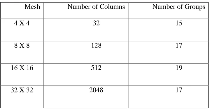
point stencil i.e the face neighbors and the neighbors of neighbors of the cell. Thus we assume here that the sparse matrix contains non zero elements corresponding to these nine neighbors and one for self and all other entries for any column should be zero. As largely the coefficient matrix is sparse, thus we need to solve only for non-zero elements of the matrix. Thus a matrix 𝑆 is formed such that,

𝑠_𝑖𝑗 = 1 𝑖𝑓 𝑖 𝑖𝑠 𝑎 𝑛𝑒𝑖𝑔𝑕𝑏𝑜𝑢𝑟 𝑜𝑟 𝑛𝑒𝑖𝑔𝑕𝑏𝑜𝑢𝑟 𝑜𝑓 𝑛𝑒𝑖𝑔𝑕𝑏𝑜𝑢𝑟 𝑡𝑜 𝑗 0 𝑜𝑡𝑕𝑒𝑟𝑤𝑖𝑠𝑒

𝐴11 𝐴12 𝐴13 0 0 0

0 𝐴22 𝐴23 𝐴24 0 0

0 0 𝐴33 𝐴34 𝐴35 0

0 0 0 𝐴44 𝐴45 𝐴46

0 0 0 0 𝐴55 𝐴56

0 0 0 0 0 𝐴66

(2.37)

𝐺𝑟𝑜𝑢𝑝 1 = 𝐶₁ + 𝐶₄ ; ; 𝐺𝑟𝑜𝑢𝑝 2 = 𝐶₂ + 𝐶₅ ; ; 𝐺𝑟𝑜𝑢𝑝 3 = 𝐶₃ + 𝐶₆

Thus the group matrix so formed is,

𝐴11 𝐴12 𝐴13 𝐴24 𝐴22 𝐴23 𝐴34 𝐴35 𝐴33 𝐴44 𝐴45 𝐴46 0 𝐴55 𝐴56

0 0 𝐴66

(2.38)

Table 2.1 Number of Columns and groups formed after CPR Algorithm

Mesh Number of Columns Number of Groups

4 X 4 32 15

8 X 8 128 17

16 X 16 512 19

32 X 32 2048 17

2.3.5 Diagonal Preconditioner

Diagonal preconditioner or jacobi preconditioner is the easiest one to employ. The diagonal elements of the coefficient matrix serve as the preconditioner matrix. The inverse of the diagonal matrix is used to obtain required preconditioning. Thus

𝑃 = 𝑎𝑖𝑖 (2.39)

2.3.6 LU-SGS Preconditioner

In Lower Upper Symmetric Gauss Seidel (LU-SGS) Preconditioner,

𝑃 = 𝐷 + 𝐿 𝐷−1 𝐷 + 𝑈 (2.40)

2.3.7 ILU Preconditioner

ILU Preconditioner is the most efficient preconditioner considered here. It is also most expensive to employ. The algorithm for implementing this preconditioner is given as suggested by Kim, Yun [31].

𝐴₀ = 𝐴 𝑓𝑜𝑟 𝑘 = 1, 𝑛 − 1

𝑁_𝑘 = 𝑛_𝑖𝑗𝑘 , 𝑤𝑕𝑒𝑟𝑒 𝑛_𝑖𝑗𝑘 = −𝑎_𝑖𝑗𝑘 𝑖𝑓 𝑘, 𝑗 ∈ 𝑃 𝑓𝑜𝑟 𝑎𝑙𝑙 𝑗 𝑠𝑢𝑐𝑕 𝑡𝑕𝑎𝑡 𝑗 > 𝑘 𝑛_𝑖𝑗𝑘 = −𝑎_𝑖𝑗 𝑘 𝑖𝑓 𝑖, 𝑘 ∈ 𝑃 𝑓𝑜𝑟 𝑎𝑙𝑙 𝑖 𝑠𝑢𝑐𝑕 𝑡𝑕𝑎𝑡 𝑖 < 𝑘

𝑛_𝑖𝑗𝑘 = 0, 𝑂𝑡𝑕𝑒𝑟𝑤𝑖𝑠𝑒 𝐴 _𝑘 = 𝑎 _𝑖𝑗𝑘 = 𝐴_𝑘−1+ 𝑁_𝑘

𝐿𝑘 = 𝑙𝑖𝑗𝑘 𝑖𝑠 𝑎𝑛 𝑒𝑙𝑒𝑚𝑒𝑛𝑡𝑜𝑟𝑦 𝑙𝑜𝑤𝑒𝑟 𝑡𝑟𝑖𝑎𝑛𝑔𝑢𝑙𝑎𝑟 𝑚𝑎𝑡𝑟𝑖𝑥

𝑤𝑕𝑒𝑟𝑒 𝑙_𝑖𝑗𝑘 = −𝑎 _𝑖𝑘𝑘 /𝑎 _𝑘𝑘𝑘 𝐴𝑘 = 𝐿𝑘𝐴 𝑘

𝐿 = (𝐿𝑛−1𝐿𝑛−2… … … . 𝐿2𝐿1)−1

𝑈 = 𝐴_{𝑛 −1}

𝑁 = 𝑁_𝑘

𝑛−1

𝑘=1

This is the ILU decomposition of coefficient matrix A. The preconditioner matrix is given as product of 𝐿 and 𝑈.

Chapter 3

An analysis of Existing Viscous Flux Formulae

Two existing cell centered finite volume schemes for viscous fluxes are analyzed in this chapter on uni-directional stretched grids. The existing schemes are compared with reconstruction scheme.

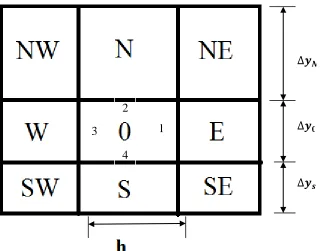
3.1 Model grid Topology and Formulae

The grid topology used for the analysis in this chapter is uni-directional stretched grid as shown in figure 3.1.

Figure 3.1 A Uni-Directional Stretched Grid

For the uni-directional stretched grid, a non-unity aspect ratio is chosen such that,

𝛿 = 𝑕 ∆𝑦₀

∆𝒚𝟎

∆𝒚_𝒔 ∆𝒚𝑵

1 1 3

𝑎𝑛𝑑, ∆𝑦𝑁 ∆𝑦0

=∆𝑦0 ∆𝑦𝑠

= 𝛽

𝛽 is the stretching ratio and 𝛿 is the aspect ratio.

The finite volume formulation of the laplace equation for an element I with volume 𝛺𝑖 give us,

∇2𝑈𝑑𝛺

𝛺𝑖

= ∇𝑈𝑑Г

Г

= ∇ 𝑈 ₁. n A1+ ∇ 𝑈 ₂. n A2+ ∇ 𝑈 ₃. n A3+ ∇ 𝑈 ₄. n A4 3.1

For the above topology considered, the laplace operator reduces to the following form.

𝐿 𝑈₀ = 1

𝑕 𝑈𝑥,𝐸− 𝑈𝑥,𝑊+ 𝛿(𝑈𝑦,𝑁 − 𝑈𝑦,𝑆) (3.2)

where, 𝑈𝑥,𝐸, 𝑈𝑥,𝑊, 𝑈𝑦,𝑁 and 𝑈𝑦 ,𝑆 are the gradients at the faces 1, 2, 3and 4 respectively as shown in figure 3.1. The calculation of the face gradients poses a major challenge today. Two approaches, introduced in chapter 2 are also discussed and analyzed here. The analysis of the scheme includes analysis on Discrete Maximum Principle (DMP), consistency and accuracy of the scheme.

3.2 Discrete Maximum Principle

Discrete Maximum Principle states that maximum of the function occur at the boundaries. Locally this means that the value at a point is bounded by the solution in the neighborhood of the point. An N point stencil is arrived at for the laplace operator as given in equation 3.3.

∇2_{𝑈 = 𝐿 𝑈 = 𝛼} 𝑛𝑈𝑛 𝑁

𝑛=0

N is the total number of points. If a stencil could be found such that the coefficients 𝛼_𝑛 are positive, then the scheme satisfies the discrete maximum principle. Locally, above equation can be solved for 𝑈0 as follows,

𝑈₀ = 𝜔_𝑛𝑈_𝑛

𝑁

𝑛=1

(3.4)

where, 𝜔𝑛 = − 𝛼𝑛

𝛼0 . To be bounded by neighbors the value 𝑈0must satisfy following condition,

min 𝑈₁, 𝑈₂, … < 𝑈₀ < max 𝑈₁, 𝑈₂, … (3.5)

The condition in equation 3.5 is satisfied if 𝜔_𝑛 ≥ 0. Thus if in the stencil all the coefficients are positive, then it satisfies Discrete Maximum Principle.

3.3 Accuracy

Consider the Laplace operator again, writing the Taylor’s expansion and collecting the partial derivative terms as in equation 3.6.

𝐿 𝑈 = (𝛼_𝑛 𝑛 ) + 𝛼_𝑛𝜁_𝑛 𝑛 𝜕𝑈 𝜕𝑥 + 𝛼𝑛𝜂𝑛 𝑛 𝜕𝑈 𝜕𝑦 +

𝛼𝑛 𝑛𝜁𝑛2

2

𝜕2𝑈 𝜕𝑥2 +

𝛼𝑛 𝑛𝜂𝑛2

2

𝜕2𝑈 𝜕𝑦2

+ ⋯ (3.6)

where, 𝜁𝑛 = 𝑥𝑛 − 𝑥0 𝑎𝑛𝑑 𝜂𝑛 = 𝑦𝑛 − 𝑦0 .

In the above equation consider the following equations,

(𝛼_𝑛

𝑛

) = 0 3.7 𝛼_𝑛𝜁_𝑛

𝑛

= 0 (3.8)

𝛼_𝑛𝜂_𝑛

𝑛

= 0 3.9 𝛼_𝑛𝜁_𝑛2

𝑛

𝛼_𝑛𝜁_𝑛𝜂_𝑛

𝑛

= 0 3.10 𝛼_𝑛𝜂_𝑛2

𝑛

= 2 (3.12)

𝛼_𝑛𝜁_𝑛3

𝑛

= 0 3.13 𝛼_𝑛𝜁_𝑛2𝜂_𝑛

𝑛

= 0 (3.14)

𝛼_𝑛𝜂_𝑛3 𝑛

= 0 3.15 𝛼_𝑛𝜂_𝑛2_𝜁 𝑛 𝑛

= 0 (3.16)

Equations 3.7 to 3.12 ensure a first order accurate scheme and equations 3.13 to 3.16 ensure second order accuracy. Thus a laplace operator can be written as,

𝐿 𝑈 = ∇2𝑈 + 𝑂 𝑕2 (3.17) 𝑂(𝑕2) denotes the higher order terms. As the higher order are of the order of 𝑕2, thus it has a second order accuracy.

3.4 Consistency

A stencil for laplace is consistent if it can be expressed as,

𝐿 𝑈 = 𝛼1𝑈𝑥+ 𝛼2𝑈𝑦 + 𝑘1𝑈𝑥𝑥 + 𝑘2𝑈𝑥𝑦 + 𝑘3𝑈𝑦𝑦 + 𝑂 𝑕2 (3.18) Such that if 𝛼₁ ≠ 0 𝑎𝑛𝑑 𝛼₂ ≠ 0, then the scheme is dangerously inconsistent. In such a case the grid convergence even to a wrong equation can never be achieved. A consistent scheme for laplace operator is obtained if 𝑘1 = 𝑘2 and 𝛼1 = 𝛼2 = 0.

3.5.1 Modified Average Gradient Method

The averaging of the neighboring cell center gradients for the gradient at the interface is the simplest approach. It leads to checkerboard instability due to odd even decoupling. If this instability is somewhat stabilized using truncation error at boundaries, it will result into non smooth solution. The solution to this problem is adopting a gradient in the direction of the vector connecting the cell centers i.e,

𝜕𝑈

𝜕𝑙_{𝐿𝑅 𝑓𝑎𝑐𝑒} =

𝑈𝑅 − 𝑈𝐿

𝑙 _𝐿𝑅 (3.19)

Finally, the gradient is computed as

∇ 𝑈 𝑓𝑎𝑐𝑒 = ∇ 𝑈 _{𝑓𝑎𝑐𝑒} − ∇ 𝑈 _{𝑓𝑎𝑐𝑒} . 𝑙_𝐿𝑅 𝑙 _𝐿𝑅 − 𝑈_𝑅 − 𝑈_𝐿 𝑙 _𝐿𝑅 𝑙_𝐿𝑅

𝑙 _𝐿𝑅 (3.20) ∇ 𝑈

𝑓𝑎𝑐𝑒 is the averaged gradient, given as an average of the cell center gradients of the neighboring cells. ∇ 𝑈

𝑓𝑎𝑐𝑒 = 0.5 ∇ 𝑈𝐿+ ∇ 𝑈𝑅 . Here ∇ 𝑈𝐿 and ∇ 𝑈𝑅 are the gradients of the elements left and right of the interface.

This method is analyzed for a uni-directional stretched mesh as in figure 3.1. For a structured

mesh, 𝑙𝐿𝑅

𝑙 𝐿𝑅 is a unit vector. Consider a face 1 in the figure 3.1, the gradients at this face using modified average approach is given as,

𝑑𝑈 𝑑𝑥 1

𝑖 + 𝑑𝑈 𝑑𝑦 ₁𝑗 =

(𝑈₁− 𝑈_𝑖)

𝑥𝑖 − 𝑥1 2+ (𝑦𝑖− 𝑦1)2

(𝑥_𝑖 − 𝑥₁)𝑖 + 𝑦_𝑖 − 𝑦₁ 𝑗 𝑥𝑖− 𝑥1 2+ (𝑦𝑖 − 𝑦1)2

(3.21)

𝑑𝑈 𝑑𝑥 ₁ =

𝑈𝑖− 𝑈1

𝑥_𝑖− 𝑥₁ =

𝑈𝑖 − 𝑈1

𝑕 3.22

𝑑𝑈

𝑑𝑦 ₁ = 0 (3.23)

𝑑𝑈 𝑑𝑥 3

= 𝑈3− 𝑈𝑖 𝑥3− 𝑥𝑖

= 𝑈𝑖 − 𝑈3

𝑕 3.24

𝑑𝑈

𝑑𝑦 ₃ = 0 (3.25)

The gradients at the upper and lower faces are computed as,

𝑑𝑈

𝑑𝑥 ₂ = 0 3.26

𝑑𝑈 𝑑𝑦 ₂ =

𝑈₂− 𝑈_𝑖 𝑦₂− 𝑦_𝑖 =

2(𝑈₂− 𝑈_𝑖)

∆𝑦_𝑖(1 + 𝛽) (3.27)

𝑑𝑈

𝑑𝑥 ₄ = 0 3.28

𝑑𝑈 𝑑𝑦 ₄ =

𝑈₄− 𝑈_𝑖 𝑦₄− 𝑦_𝑖 =

2(𝑈₂− 𝑈_𝑖)𝛽

∆𝑦_𝑖(1 + 𝛽) (3.29)

Substituting the expressions for the interface gradients i.e. equations 3.22 to 3.29 in the equation 3.2 for the laplace operator and writing laplace equation in discretized form by collecting coefficients as,

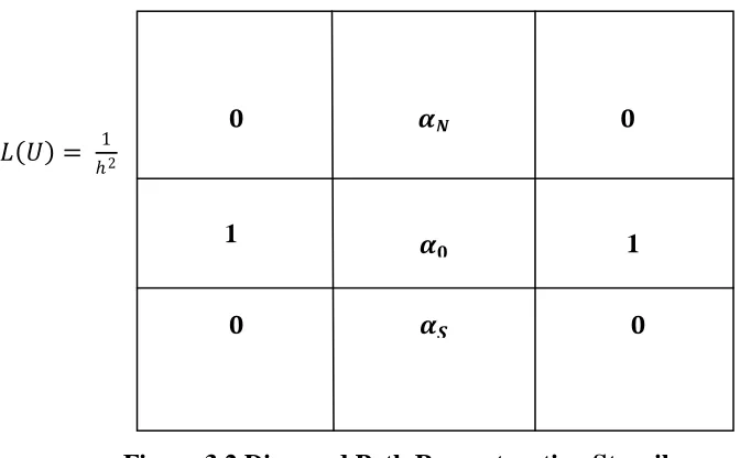
𝐿 𝑈 = 𝑈𝑊+ 𝑈𝐸 + 𝛼0𝑈0+ 𝛼𝑁𝑈𝑁+ 𝛼𝑆𝑈𝑆 (3.30) We obtain following stencil as in figure 3.2,

𝛼₀ = −2 1 + 𝛿2 𝛼_𝑁 = 2𝛿

2

𝐿 𝑈 = 1

𝑕2

Figure 3.2 Diamond Path Reconstruction Stencil

The consistency of the scheme is checked by substituting face gradients from equation 3.22 to 3.29 into equation 3.2 and Taylor’s expressions are also substituted for neighboring cells, thus we obtain the laplace equation as,

L U = Uxx +

(1 + β)2 4β Uyy +

h 1 + β 3(β − 1)

24δβ Uyyy + ⋯ (3.32)

Comparing the above equation with equation 3.18 we can write α1 = α2 = 0. Thus the scheme is not dangerously inconsistent. Also k1 ≠ k2 for β ≠ 1 thus it shows that the scheme is inconsistent for uni-directionally stretched mesh.

3.5.2 Green Gauss Reconstruction using Diamond Path Approach

Another approach for gradient calculation at the interface is presented in which a diamond path is created by connecting the vertices of the face with the centroid of the two neighboring cells. An interpolation is done for estimating the values at the vertices using the centroidal values. For this a simple approach of taking the average of the values of the neighboring cell centroid is taken.

𝜶_𝑺 𝜶_𝟎

𝜶𝑵 𝟎

1

𝟎 𝟎

𝟎

Figure 3.3 Simple Averaging Procedures at Subtended Vertex.

Thus at vertex R, 𝑈_𝑅 = 1/4(𝑈_𝑁+ 𝑈₀+ 𝑈_𝑁𝐸 + 𝑈_𝑆𝐸), and for vertex L the value is given as, 𝑈𝐿 = 1/4(𝑈𝑁+ 𝑈0+ 𝑈𝑁𝑊+ 𝑈𝑆𝑊), An improvement in the scheme is observed by using the linearly preserving weighting to find the values at the vertices. The value of the physical property is evaluated at the vertices using interpolation. The interpolation is supported by a set of elements that share a particular vertex. The value of the flow property at the vertex (𝑣_𝑖) is given as,

𝑈_𝑣𝑖 = 𝜁𝑗𝑈𝑗

𝑁_𝑣𝑖 𝑗 =1

𝜁𝑗 𝑁_𝑣𝑖 𝑗 =1

(3.33)

where 𝑈_𝑗 represents the value at the cell 𝛺_𝑗. 𝑁_𝑣𝑖 is the number of neighbors surrounding vertex 𝑣_𝑖. 𝜁_𝑗 are the dimensionless weights given as,

𝜁𝑗 = 1 + 𝜆𝑥 𝑥𝑗 − 𝑥𝑣𝑖 + 𝜆𝑦 𝑦𝑗 − 𝑦𝑣𝑖 (3.34)

𝜆_𝑥 = 𝐼𝑥𝑦𝑅𝑦 − 𝐼𝑦𝑦𝑅𝑥

𝐼_𝑥𝑦𝐼_𝑦𝑦 − 𝐼_𝑥𝑦2 ; 𝜆𝑦 =

𝐼_𝑥𝑦𝑅_𝑦 − 𝐼_𝑥𝑥𝑅_𝑥 𝐼_𝑥𝑦𝐼_𝑦𝑦 − 𝐼_𝑥𝑦2

And the moments 𝑅_𝑥, 𝑅_𝑦, 𝐼_𝑥𝑥, 𝐼_𝑥𝑦 and 𝐼_𝑦𝑦 are defined as follows, R L

NE N

NW

SE 0

𝑅_𝑥 = (𝑥_𝑗 − 𝑥_𝑣𝑖) 𝑁_𝑣𝑖 𝑗 =1 , 𝑅_𝑦 = (𝑦_𝑗 − 𝑦_𝑣𝑖) 𝑁_𝑣𝑖 𝑗 =1

𝐼_𝑥𝑥 = (𝑥_𝑗 − 𝑥_𝑣𝑖)2 𝑁_𝑣𝑖

𝑗 =1

, 𝐼_𝑥𝑥 = (𝑦_𝑗 − 𝑦_𝑣𝑖)2 𝑁_𝑣𝑖

𝑗 =1

, 𝐼_𝑥𝑥 = 𝑥_𝑗 − 𝑥_𝑣𝑖 (𝑦_𝑗 − 𝑦_𝑣𝑖)

𝑁_𝑣𝑖

𝑗 =1

The laplace operator for a single vertex is expressed as,

𝐿 𝑈₀ = 𝜁_𝑖 𝑈_𝑖 − 𝑈₀

𝑖

= 0

Using the above relation, equation 3.33 can be easily obtained for computing the value at the vertex. The gradients at the faces are found using following equation,

𝑈𝑥= 1 𝛺

𝑛1,𝑥+ 𝑛2,𝑥

2 𝑈𝑇+

𝑛2,𝑥+ 𝑛3,𝑥

2 𝑈𝐿+

𝑛3,𝑥+ 𝑛4,𝑥

2 𝑈𝐵+

𝑛4,𝑥+ 𝑛1,𝑥

2 𝑈𝑅 (3.35)

where, 𝑛1,𝑥, 𝑛1,𝑥, 𝑛1,𝑥 and 𝑛1,𝑥 are normal as shown in figure 3.4.

Figure 3.4 Sample Reconstruction Diamond Path

For uniform grids, equation 3.35 reduces to a simple central differencing equation making the scheme consistent due to fortunate geometric cancellations but for uni-directionally

𝑛 1

𝑛 4

𝑛 3

stretched grids it’s not so straight forward. The interfacial gradients are substituted in the discretized laplace equation 3.2 and the laplace equation is written as in equation 3.30 by collecting coefficients, which gives the stencil as in figure 3.5,

𝐿 𝑈 = 1

𝑕2

Figure 3.5 Stencil for Diamond Path Reconstruction on Uni-Directional Stretched Grids

𝛼0 = −2 1 + 𝛿2

𝛼_𝑁 = 2𝛿

2

1 + 𝛽 𝛼𝑆 = 𝛽𝛼𝑁

Substituting the above coefficients in N point stencil, we obtain the expression for laplace operator as,

𝐿 𝑈 = ∇2_{𝑈 = 𝑈} 𝑥𝑥 +

(1 + 𝛽)2 4𝛽 𝑈𝑦𝑦 +

𝑕 1 + 𝛽 3(𝛽 − 1)

24𝛿𝛽 𝑈𝑦𝑦𝑦 + ⋯ (3.36)

From the equation 3.36, consistency is obtained only if 𝛽 = 1 i.e for a uniform grid. For other values of 𝛽, i.e. for any uni directional stretched grid the scheme is not consistent.

0

𝜶

_𝒔

𝜶

_𝟎

𝜶

_𝑵

0

0

0

Comparing equation 3.36 and equation 3.18 can see that 𝛼₁ = 𝛼₂ = 0, thus the scheme is not dangerously inconsistent.

Both the approaches discussed above have shown identical behavior. They are consistent for uniform grids but for uni-directional stretched grids both the schemes display inconsistency. The diamond path approach is not grid transparent and also not compact as it involves vertex neighbors of each element. A comparative study done in the next section, shows that the order of accuracy of the modified gradient approach is even lesser than second order for non uniform and non regular grids.

Diamond path without linear preserving, is dangerously inconsistent while with linearly preserving at least local grid convergence can be achieved but consistency is not guaranteed although positivity is maintained. Hence next discussed is a technique which is second order accurate, consistent for uniform meshes, grid transparent and doesn’t violate DMP.

3.6 Reconstruction Scheme

In the work presented here reconstruction scheme is used to estimate the gradients at the cell interfaces. This requires calculating the gradients at the cell centers of the neighboring cells. An analysis is presented here of the reconstruction scheme on 1D non uniform grids.

Figure 3.6 1D Uni-Directionally Stretched Mesh

Above grid is chosen such that it is a uni-directional stretched grid. Thus for 𝛽 as the stretching ratio,

∆𝑥_𝑖+1 ∆𝑥𝑖

= ∆𝑥𝑖 ∆𝑥𝑖−1

= 𝛽 (3.37)

Gradients at the cell centers are given by the extrapolation of the cell center values to the neighboring cells.

𝑈_𝑖+1 = 𝑈_𝑖+ 𝑑𝑢

𝑑𝑥 _𝑖 𝑥𝑖+1− 𝑥𝑖 (3.38)

𝑈𝑖−1 = 𝑈𝑖+

𝑑𝑢 𝑑𝑥 𝑖

𝑥𝑖−1− 𝑥𝑖 (3.39)

From Figure 3.6,

𝑥_𝑖+1− 𝑥_𝑖 = 0.5 ∆𝑥_𝑖+ ∆𝑥_𝑖+1 = (∆𝑥_𝑖/2)(1 + 𝛽) 𝑎𝑛𝑑

𝑥𝑖−1 − 𝑥𝑖 = 0.5 ∆𝑥𝑖−1+ ∆𝑥𝑖 = −(

∆𝑥_𝑖 2 )

1 𝛽+ 1

Above least squares problem is solved only for one variable thus giving the cell center gradient as,

𝑑𝑈 𝑑𝑥 𝑖

= 2𝛽(𝛽 𝑈𝑖+1− 𝑈𝑖 − 𝑈𝑖−1− 𝑈𝑖) ∆𝑥𝑖 1 + 𝛽 (1 + 𝛽2)

(3.40)

Writing, similar equations for other cells and computing the cell center gradients,

𝑑𝑈

𝑑𝑥 _𝑖+1 =

2(𝛽 𝑈𝑖+2− 𝑈𝑖+1 − 𝑈𝑖 − 𝑈𝑖+1)

∆𝑥_𝑖 1 + 𝛽 (1 + 𝛽2₎ (3.41)

𝑑𝑈

𝑑𝑥 _𝑖−1 =

2𝛽2(𝛽 𝑈𝑖− 𝑈𝑖−1 − 𝑈𝑖−2 − 𝑈𝑖−1)

∆𝑥_𝑖 1 + 𝛽 (1 + 𝛽2₎ (3.42)

𝑈_𝑖𝑖+1𝑑𝛺_𝑖1= 𝑈_𝑖𝑑

𝛺𝑖

𝛺_𝑖

𝛺𝑖1

+ 𝑈_𝑖+1𝑑

𝛺𝑖+1

𝛺_𝑖+1 (3.43)

𝑈𝑖𝑖+1 =

𝑈_𝑖𝛺_𝑖 + 𝑈_𝑖+1𝛺_𝑖+1 𝛺𝑖 + 𝛺𝑖+1

= 𝑈𝑖∆𝑥𝑖 + 𝑈𝑖+1∆𝑥𝑖+1 ∆𝑥𝑖 + ∆𝑥𝑖+1

= 𝑈𝑖+ 𝑈𝑖+1𝛽

1 + 𝛽 (3.44)

𝑥_𝑖𝑖+1 = 𝑥𝑖𝛺𝑖 + 𝑥𝑖+1𝛺𝑖+1 𝛺_𝑖 + 𝛺_𝑖+1 =

𝑥_𝑖∆𝑥_𝑖+ 𝑥_𝑖+1∆𝑥_𝑖+1 ∆𝑥_𝑖 + ∆𝑥_𝑖+1 =

𝑥_𝑖+ 𝑥_𝑖+1𝛽

1 + 𝛽 (3.45)

Extrapolation of the centroidal value of the union to the cell center values of the neighboring cells is done as following equations,

𝑈_𝑖 = 𝑈_𝑖𝑖+1+ 𝑑𝑈

𝑑𝑥 _𝑖𝑖+1 𝑥𝑖− 𝑥𝑖𝑖+1 (3.46)

∆𝑥_𝑖 𝑑𝑈

𝑑𝑥 _𝑖𝑖+1 = ∆𝑥𝑖 𝑑𝑈𝑑𝑥 _𝑖 (3.47)

𝑈_𝑖+1 = 𝑈_𝑖𝑖+1+ 𝑑𝑈

𝑑𝑥 _𝑖𝑖+1 𝑥𝑖+1− 𝑥𝑖𝑖+1 (3.48)

∆𝑥_𝑖+1 𝑑𝑈

Thus the over-determined system is solved for just one variable. Thus the gradient at the interface is obtained as in equation 3.50 and equation 3.51.

𝑑𝑈 𝑑𝑥 𝑖𝑖+1

=2(𝑈𝑖+1− 𝑈𝑖) 5 1 + 𝛽 ∆𝑥𝑖

+ 8𝛽(𝛽 𝑈𝑖+1− 𝑈𝑖 − (𝑈𝑖−1− 𝑈𝑖) 5 1 + 𝛽 (1 + 𝛽2₎2_∆𝑥

𝑖

+ 8𝛽

2_{(𝛽 𝑈}

𝑖+2− 𝑈𝑖+1 − (𝑈𝑖− 𝑈𝑖+1)

5 1 + 𝛽 (1 + 𝛽2₎2_∆𝑥 𝑖

(3.50)

𝑑𝑈 𝑑𝑥 𝑖𝑖−1

= 2(𝑈𝑖− 𝑈𝑖−1)𝛽 5 1 + 𝛽 ∆𝑥𝑖

+ 8𝛽

3_{(𝛽 𝑈}

𝑖+1− 𝑈𝑖 − (𝑈𝑖−1− 𝑈𝑖)

5 1 + 𝛽 (1 + 𝛽2₎2_∆𝑥 𝑖

+ 8𝛽

2_{(𝛽 𝑈}

𝑖− 𝑈𝑖−1 − (𝑈𝑖−2− 𝑈𝑖−1)

5 1 + 𝛽 (1 + 𝛽2₎2_∆𝑥 𝑖

(3.51)

Finite volume formulation of the laplace equation gives,

𝑑

2_𝑈

𝑑𝑥2 𝑖

𝑑𝛺_𝑖 = 𝑑𝑈

𝑑𝑥 _𝑖𝑖+1 ∆xi −

𝛺𝑖

𝑑𝑈

𝑑𝑥 _𝑖𝑖−1 ∆xi (3.52)

Thus, 𝑑 2_𝑈 𝑑𝑥2 𝑖 𝑑𝛺𝑖= 2 5 1 + 𝛽 ∆𝑥𝑖

((𝑈𝑖+1− 𝑈𝑖) 𝛺𝑖

− (𝑈𝑖− 𝑈𝑖−1)) +

8𝛽 𝛽 𝑈𝑖+1− 𝑈𝑖 − 𝑈𝑖−1− 𝑈𝑖 1 − 𝛽2

5 1 + 𝛽 1 + 𝛽22_∆𝑥 𝑖

+8𝛽

2_{(𝛽 𝑈}

𝑖+2− 𝑈𝑖+1 − 𝑈𝑖− 𝑈𝑖+1 − 𝛽 𝑈𝑖− 𝑈𝑖−1 + (𝑈𝑖−2− 𝑈𝑖−1))

5 1 + 𝛽 1 + 𝛽22_∆𝑥 𝑖

(3.53)

Substituting following Taylor’s expansions,

𝑈_𝑖+1 = 𝑈_𝑖 + 𝑑𝑈

𝑑𝑥 _𝑖 𝑥𝑖+1− 𝑥𝑖 + 𝑑2𝑈 𝑑𝑥2 𝑖

𝑥𝑖+1− 𝑥𝑖

2

2

+ 𝑂 𝑕2 _(3.54)

𝑈𝑖−1 = 𝑈𝑖+

𝑑𝑈 𝑑𝑥 𝑖

𝑥𝑖−1 − 𝑥𝑖 +

𝑑2𝑈 𝑑𝑥2 𝑖

𝑥_𝑖−1 − 𝑥_𝑖 2

2

+ 𝑂 𝑕2 (3.55)

𝑈_𝑖+2 = 𝑈_𝑖+ 𝑑𝑈

𝑑𝑥 _𝑖 𝑥𝑖+2 − 𝑥𝑖 + 𝑑2_𝑈

𝑑𝑥2 𝑖

𝑥𝑖+2 − 𝑥𝑖

2

2

𝑈_𝑖−2 = 𝑈_𝑖+ 𝑑𝑈

𝑑𝑥 _𝑖 𝑥𝑖−2− 𝑥𝑖 + 𝑑2_𝑈

𝑑𝑥2

𝑥_𝑖−2− 𝑥_𝑖 2

2

+ 𝑂 𝑕2 (3.57)

Substituting the expansions from 3.54 to 3.57 in equation 3.53, we obtain,

∇2_{𝑈 = 0} 𝑑𝑈 𝑑𝑥+

𝑑2_𝑈(∆𝑥 𝑖) 𝑑𝑥2

(1 + 𝛽)2

20𝛽 +

1 + 𝛽 𝛽3_{− 1 (1 − 𝛽}2₎ 5𝛽(1 + 𝛽2₎2

+ (1 + 𝛽)

5𝛽2_{(1 + 𝛽}2₎ 𝛽 (1 + 𝛽)

2_{− 1 +} 1

𝛽2 + 1 +

(1 + 𝛽)2

𝛽4 −

1

𝛽2 (3.58)

Chapter 4

Numerical Experiments

Numerical experiments were carried out in this work on various meshes. The results for assessment of accuracy with different diffusion tensors are presented here. These are followed by the accuracy study on distorted meshes. In the following subsection, the scheme is tested for its robustness on heterogeneous diffusion tensor. Further, a study is also carried out to determine the convergence of the preconditioned GMRES solver. A comparison is made between the reconstruction scheme and modified average gradient method. Four kinds of meshes are used to carry out the experiments. Figure 4.1 demonstrates the regular triangular, unstructured and anisotropic meshes while figure 4.9 shows the distorted meshes used. In the presented work some experiments are carried out with known exact solutions. Thus error estimation was done by L2 norm as given in equation 4.1.

𝑈_𝑕 − 𝑈 _𝐿2 = (𝑈_𝑖𝑁𝑢𝑚𝑒𝑟𝑖𝑐 𝑎𝑙 − 𝑈_𝑖𝐸𝑥𝑎𝑐𝑡)2 𝑁

𝑖=1

𝛺_𝑖 (4.1)

where, N is the number of elements. 𝑈𝑕 is the numerical solution and U is the exact solution.

4.1 Assessment of Condition Number

𝐶𝑁 = 𝐴 𝐴 −1 _(4.2) For better conditioning the non normalized form is used as given by equation 2.12. Similarly the normalization of the system is done for calculation of the gradients at the cell interfaces. A comparison is also made between the condition numbers of normalized and non-normalized forms of matrix. Following are the results for condition number for calculation of cell center gradients.

Table 4.1 Condition Numbers for Gradient at Cell Centers for Regular Triangular Meshes

Triangular Mesh 4 X 4 Mesh 8 X 8 Mesh 16 X 16 Mesh 32 X 32 Mesh

Non-Normalized 2.766 2.766 2.766 2.766

Normalized 1.500 1.500 1.500 1.500

Table 4.2 Condition Numbers for Gradient at Cell Centers for Unstructured Meshes Stretched Mesh Coarse Mesh Medium Mesh Fine Mesh Very Fine

Mesh

Non-Normalized 5.158 8.260 16.188 31.789

Normalized 3.254 3.211 3.319 3.500

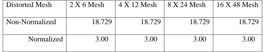
Table 4.3 Condition Numbers for Gradient at Cell Centers for Anisotropic Meshes Distorted Mesh 2 X 6 Mesh 4 X 12 Mesh 8 X 24 Mesh 16 X 48 Mesh

Non-Normalized 18.729 18.729 18.729 18.729

Thus we observe that the normalized matrix gives better conditioning. Similarly the condition number is calculated for the cell interfaces by forming the least squares problem using reconstruction equations 2.18 to 2.23.

Table 4.4 Condition Numbers for gradient at cell interfaces for Regular Triangular Meshes

N by N Mesh 4 X 4 Mesh 8 X 8 Mesh 16 X 16 Mesh 32 X 32 Mesh

Non-Normalized 1.138 1.138 1.138 1.138

Normalized 1.138 1.138 1.138 1.138

Table 4.5 Condition Numbers for gradient at cell interfaces for Anisotropic Meshes Stretched

Mesh

2 X 6 Mesh

4 X 12 Mesh

8 X 24 Mesh

16 X 48 Mesh

Non-Normalized 9.762 9.762 9.762 9.762

Normalized 9.762 9.762 9.762 9.762

Table 4.6 Condition Numbers for gradient at cell interfaces for Unstructured Meshes Unstructured Coarse Mesh Medium Mesh Fine Mesh Very Fine Mesh

Non-Normalized 2.961 5.172 11.215 22.082

The condition number shows that in case of unstructured meshes the normalized approach decreases the condition number thus it is more beneficial than using non-normalized approach.

4.2 Positivity Study

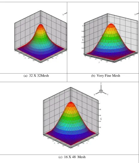
In this test case it is shown that our scheme does not violate the Discrete Maximum Principle. Different meshes are tried here with different triangulations and the positivity is found to be maintained in all the cases. The analytical solution is not known in this case. Homogeneous Dirichlet boundary condition is applied. The meshes used for the positivity study are shown in figure 4.1. The results obtained on different types of mesh are given in figure 4.2. In this study we consider diffusion problem as in equation 2.1, in the unit square Ω = (0, 1)2. In this study it was shown that the function attains a minimum value of zero at the boundaries. Thus the positivity is maintained throughout the domain.

4.2.1 Test Case 1 a) Source Term

𝑓 𝑥, 𝑦 = 1 𝑖𝑓 𝑥, 𝑦 ∈ 3/8,5/8 2

0 𝑂𝑡𝑕𝑒𝑟𝑤𝑖𝑠𝑒 (4.3)

b) Diffusion Tensor

𝐷 = 𝑦

2_{+ 𝜀𝑥}2 _{− 1 − 𝜀 𝑥𝑦}

− 1 − 𝜀 𝑥𝑦 𝜀𝑦2+ 𝑥2 , 𝜀 = 5 × 10

−2 _(4.4)

c) Analytical Function

𝑁𝑜𝑡 𝐾𝑛𝑜𝑤𝑛

(a) 32 X 32Mesh (b) Very Fine Mesh

(c) 16 X 48 Mesh

(a) 32 X 32Mesh (b) Very Fine Mesh

(c) 16 X 48 Mesh