Semiparametric Bayesian Quantile Regression.

(1)

ABSTRACT

JANG, WOO SUNG. Semiparametric Bayesian Quantile Regression. (Under the direction of Huixia Judy Wang.)

We propose semiparmetric Bayesian quantile regression methods for analyzing inde-pendent and clustered data and Bayesian regularized quantile regression methods for quantile and interquantile shrinkage.

Bayesian quantile regression is challenging without making any parametric likelihood assumptions. Instead of posing any parametric distributional assumptions on the ran-dom errors, we approximate the central density by linearly interpolating the conditional quantile functions of the response at multiple quantiles and estimate the tail densities by adopting extreme value theory.

In Chapter 2, we propose a semiparametric Bayesian quantile regression method for analyzing independent data based on the proposed approximate likelihood. In Chapter 3, we develop a semiparametric Bayesian quantile regression method for analyzing clustered data, where random effects are included to accommodate the intra-cluster dependence. Through joint-quantile modeling, the proposed methods yield the joint posterior distri-bution of quantile coefficients at multiple quantiles and meanwhile avoid the quantile crossing issue. Through simulation studies, we demonstrate that the proposed methods lead to more efficient multiple-quantile estimation than existing methods for quantile regression in finite samples.

(2)

(3)

Semiparametric Bayesian Quantile Regression

by

Woo Sung Jang

A dissertation submitted to the Graduate Faculty of North Carolina State University

in partial fulfillment of the requirements for the Degree of

Doctor of Philosophy

Statistics

Raleigh, North Carolina 2014

APPROVED BY:

Sujit Ghosh Daowen Zhang

Wenbin Lu Huixia Judy Wang

(4)

BIOGRAPHY

(5)

ACKNOWLEDGEMENTS

First I would like to express my first and deepest gratitude to Dr. Huixia Wang for her excellent guidance, patience, financial and emotional support. I could not have imagined having a better mentor for my Ph.D. study.

I am especially thankful to my committee members, Dr. Sujit Ghosh, Dr. Daowen Zhang and Dr. Wenbin Lu for joining my committee. I greatly appreciate constructive feedback they have provided. I also thank Dr. Ratna Sharma-Shivappa for serving on my committee as the graduate school representative.

(6)

LIST OF TABLES

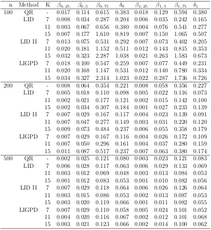
Table 2.1 Mean squared errors of parameter estimators for data generated from model (2.9) withi ∼N(0,1) from the conventional quantile regression method (QR), the LID method of Feng (LID) based on the “optimal”σ, the LID method with the proposed variance parameter selection method (LID II) and the proposed LIGPD method using GPD tail density ap-proximation (LIGPD), where δ0=β0,.75−β0,.5 and δ1=β1,.75−β1,.5. . . 27

Table 2.2 Mean squared errors of parameter estimators for data generated from model (2.9) with i ∼ t3 from the conventional quantile regression

method (QR), the LID method of Feng (LID) based on the “optimal”σ, the LID method with the proposed variance parameter selection method (LID II) and the proposed LIGPD method using GPD tail density ap-proximation (LIGPD), where δ0=β0,.75−β0,.5 and δ1=β1,.75−β1,.5. . . 28

Table 2.3 Mean squared errors of parameter estimators for data generated from model (2.9) with i ∼ χ21 from the conventional quantile regression

method (QR), the LID method of Feng (LID) based on the “optimal”σ, the LID method with the proposed variance parameter selection method (LID II) and the proposed LIGPD method using GPD tail density ap-proximation (LIGPD), where δ0=β0,.75−β0,.5 and δ1=β1,.75−β1,.5. . . 29

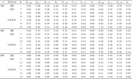
Table 2.4 Quantile crossing rates in percentage (%) for data generated from model (2.9) with i ∼ N(0,1), t3, and χ21 from the conventional quantile

re-gression method. . . 33 Table 2.5 Coverage probabilities (%) of 95% credible intervals (LIGPD) and 95%

confidence intervals (QR), where xi ∼ LN(0,1), δ0=β0,.75 - β0,.5 and

δ1=β1,.75 -β1,.5. . . 34

Table 2.6 Mean squared errors of parameter estimators for data generated from model (2.12) withi ∼N(0,1) from the conventional quantile regression method (QR), the LID method of Feng (LID) based on the “optimal”σ, the proposed LID method (LIGPD), whereδ0=β0,.75−β0,.5,δ1=β1,.75−

β1,.5 and δ2=β2,.75−β2,.5. . . 36

Table 2.7 Mean squared errors of parameter estimators for data generated from model (2.12) with i ∼ t4 from the conventional quantile regression

method (QR), the LID method of Feng (LID) based on the “optimal” σ, the proposed LID method (LIGPD), whereδ0=β0,.75−β0,.5,δ1=β1,.75−

β1,.5 and δ2=β2,.75−β2,.5. . . 39

(9)

Table 3.1 Mean squared error of parameter estimators at median for the data generated from model (3.4) and (3.5) from the LIGPD, REML and ALD method. The REML estimators are grayed out when it cannot be directly compared to LIGPD and ALD. . . 54 Table 3.2 Relative efficiency of the LIGPD, ALD and BEL estimators at

me-dian with respect to the REML estimator at meme-dian. Relative efficiency larger than 1 means the competing method has smaller MSE and thus higher efficiency than the REML estimator. The results for BEL were from Table 3 in Kim and Yang (2011). . . 56 Table 3.3 Mean squared error of parameter estimators at median for the data

generated from model (3.4) and (3.5) from the LIGPD, REML and ALD method. The REML estimators are grayed out when it cannot be directly compared to LIGPD and ALD. . . 57 Table 3.4 Relative efficiency of the LIGPD, ALD and BEL estimators at

me-dian with respect to the REML estimator at meme-dian. Relative efficiency larger than 1 means the competing method has smaller MSE and thus higher efficiency than the REML estimator. The results for BEL were from Table 3 in Kim and Yang (2011). . . 59 Table 3.5 Mean squared errors of LIGPD and ALD estimators atτ = 0.1,· · · ,0.9

for data generated from model (3.4) withij ∼N(0,1). . . 60 Table 3.6 Mean squared errors of LIGPD and ALD estimators atτ = 0.1,· · · ,0.9

for data generated from model (3.5) withij ∼N(0,1). . . 62 Table 3.7 Mean squared errors of LIGPD and ALD estimators atτ = 0.1,· · · ,0.9

for data generated from model (3.4) withij ∼t2. . . 63

Table 3.8 Mean squared errors of LIGPD and ALD estimators atτ = 0.1,· · · ,0.9 for data generated from model (3.5) withij ∼t2. . . 64

Table 3.9 Mean squared errors of LIGPD and ALD estimators atτ = 0.1,· · · ,0.9 for data generated from model (3.4) withij ∼LN(0,1). . . 65 Table 3.10 Mean squared errors of LIGPD and ALD estimators atτ = 0.1,· · · ,0.9

for data generated from model (3.5) withij ∼LN(0,1). . . 66 Table 3.11 Quantile crossing rates in percentage (%) of the ALD estimators at

τ = 0.1,· · · ,0.9 for data generated from model (3.4) and (3.5) . . . 67 Table 3.12 Mean squared errors of LIGPD and ALD estimators atτ = 0.1,· · · ,0.9

for data generated from model (3.7) withij ∼N(0,1). For the LIGPD method, the estimates of random-effect variance parameters are con-stant across quantile levels. . . 70 Table 3.13 Mean squared errors of LIGPD and ALD estimators atτ = 0.1,· · · ,0.9

(10)

Table 3.14 Mean squared errors of LIGPD and ALD estimators atτ = 0.1,· · · ,0.9 for data generated from model (3.7) withij ∼χ21. . . 74

Table 3.15 Quantile crossing rates in percentage (%) of the ALD estimators at τ = 0.1,· · · ,0.9 for data generated from model (3.7). . . 74 Table 4.1 A thousand times the mean of integrated squared errors (103× MISE)

across 500 simulations for data generated from model (4.6) from the con-ventional quantile regression method (QR), the Bayesian fused adaptive LASSO (BFLL), the Bayesian fused adaptive LASSO II (BFGLL) and the Bayesian fused adaptive group LASSO (BFGLGL). The values in the parentheses are the standard errors of 103_× _{MISE. . . .} ₉₉

Table 4.2 102×bias of ˆβl,τ, l= 0,1,2,3 from the QR, BFLL, BFGLL and BFGLGL estimators in model (4.6) withh(xi1) = 1. . . 105

Table 4.3 A thousand times the mean of integrated squared errors (103_× _MISE)

for data generated from model (4.7) from the conventional quantile regression method (QR), the Bayesian fused adaptive LASSO (BFLL), the Bayesian fused adaptive LASSO II (BFGLL) and the Bayesian fused adaptive group LASSO (BFGLGL). The values in the parentheses are the standard errors of 103_×_{MISE. . . 107}

Table 4.4 A thousand times the mean of integrated squared errors (103_× _MISE)

for data generated from model (4.8) from the conventional quantile regression method (QR), the Bayesian fused adaptive LASSO (BFLL), the Bayesian fused adaptive LASSO II (BFGLL) and the Bayesian fused adaptive group LASSO (BFGLGL). The values in the parentheses are the standard errors of 103_×_{MISE. . . 111}

Table A.1 Mean squared errors of parameter estimators for data generated from model (2.9) with i ∼ N(0,1), t3 or χ21 from the proposed LIGPD

method with updating the scale and shape parameters, whereδ0=β0,.75−

β0,.5 and δ1=β1,.75−β1,.5. . . 132

Table A.2 Mean squared errors of parameter estimators for data generated from model (2.9) with i ∼ N(0,1), t3 or χ21 from the proposed LIGPD

method with simpler constraint, whereδ0=β0,.75−β0,.5andδ1=β1,.75−β1,.5.133

Table A.3 Mean squared errors of parameter estimators for data generated from model (2.9) with i ∼ N(0,1), t3 or χ21 from the proposed LID method

with matching linearly interpolated density and truncated normal den-sity, whereδ0=β0,.75−β0,.5 and δ1=β1,.75−β1,.5. . . 134

(11)

LIST OF FIGURES

Figure 1.1 The density function of W = U V, where U and V are independent standard normal random variables. . . 7 Figure 2.1 The LID estimates for data sets generated from N(0,1) and χ2

3. The

dashed curves are the true density functions and the solid lines are the LID estimations to N(0,1) (the left plot) and χ2₃ (the right plot) . . . 16 Figure 2.2 The estimated upper tail densities for random samples of size 100 and

200 from the standard normal distribution. The horizontal axis repre-sentsz and the vertical axis represents the density. The dotted vertical lines arez = ˆΦ−1_{(0.85). The solid curves are the true density and the}

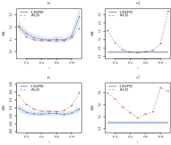
dotted curves correspond to the GPD tail approximation. . . 23 Figure 2.3 Mean squared errors of the QR, LID, LID II and LIGPD estimators

for data generated from model (2.9) with i ∼ N(0,1). The shaded bands represent the range of MSEs of the LID estimator with σ = 0.5,1,1.5,2,3. . . 30 Figure 2.4 Mean squared errors of the QR, LID, LID II and LIGPD estimators

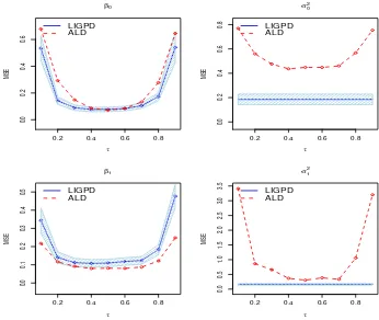
for data generated from model (2.9) with i ∼ t3. The shaded bands

represent the range of MSEs of the LID estimator withσ = 0.5,1,1.5,2,3. 31 Figure 2.5 Mean squared errors of the QR, LID, LID II and LIGPD estimators

for data generated from model (2.9) with i ∼ χ21. The shaded bands

represent the range of MSEs of the LID estimator with σ1 = 0.5 and

σ2 = 1,2,3,4,5. . . 32

Figure 2.6 MSE of the QR, LID and LIGPD estimators for data generated from model (2.12) withi ∼N(0,1), whereδ0=β0,.75−β0,.5,δ1=β1,.75−β1,.5

and δ2=β2,.75−β2,.5. The shaded bands represent the range of MSEs

of the LID estimator with σ= 0.5,1,1.5,2,3. . . 37 Figure 2.7 MSE of the QR, LID and LIGPD estimators for data generated from

model (2.12) with i ∼t4, where δ0=β0,.75−β0,.5, δ1=β1,.75−β1,.5 and

δ2=β2,.75−β2,.5. The shaded bands represent the range of MSEs of the

LID estimator withσ = 0.5,1,1.5,2,3. . . 38 Figure 3.1 Mean squared error of parameter estimators at median for three models

with homoscedastic errors (N1: N(0,1), T1: t2, LN1: LN(0,1)) and

three models with heteroscedastic errors (N2: N(0,1), T2: t2, LN2:

(12)

Figure 3.2 Mean squared error of parameter estimators at median for three models with homoscedastic errors (N1: N(0,1), T1: t2, LN1: LN(0,1)) and

three models with heteroscedastic errors (N2: N(0,1), T2: t2, LN2:

LN(0,1)) from the LIGPD (solid), REML (dotted) and ALD (dashed) methods. . . 58 Figure 3.3 Mean squared errors of LIGPD and ALD estimators atτ = 0.1,· · · ,0.9

for data generated from model (3.4) with ij ∼ N(0,1). MSE of β0,.5

(top left), β1,.5 (bottom left), σ02 (top right) and σ20 (bottom right) of

LIGPD (solid line) and ALD (dashed line). The horizontal axis repre-sents quantile levels and the vertical axis reprerepre-sents MSE. The shaded bands represent 95% confidence bands of MSE of the LIGPD estima-tor. For the LIGPD method, the estimates of random-effect variance parameters are constant across quantile levels. . . 61 Figure 3.4 Mean squared errors of LIGPD and ALD estimators atτ = 0.1,· · · ,0.9

for data generated from model (3.5) withij ∼N(0,1). . . 62 Figure 3.5 Mean squared errors of LIGPD and ALD estimators atτ = 0.1,· · · ,0.9

for data generated from model (3.4) withij ∼t2. . . 63

Figure 3.6 Mean squared errors of LIGPD and ALD estimators atτ = 0.1,· · · ,0.9 for data generated from model (3.5) withij ∼t2. . . 64

Figure 3.7 Mean squared errors of LIGPD and ALD estimators atτ = 0.1,· · · ,0.9 for data generated from model (3.4) withij ∼LN(0,1). . . 65 Figure 3.8 Mean squared errors of LIGPD and ALD estimators atτ = 0.1,· · · ,0.9

for data generated from model (3.5) withij ∼LN(0,1). . . 66 Figure 3.9 Mean squared errors of LIGPD and ALD estimators atτ = 0.1,· · · ,0.9

for data generated from model (3.7) withij ∼N(0,1). The solid line is for LIGPD and the dashed line is for ALD. The shaded region indicates 95% pointwise confidence bands of the MSE of the LIGPD estimators. 71 Figure 3.10 Mean squared errors of LIGPD and ALD estimators atτ = 0.1,· · · ,0.9

for data generated from model (3.7) withij ∼t3. The solid line is for

LIGPD and the dashed line is for ALD. The shaded region indicates 95% pointwise confidence bands of the MSE of the LIGPD estimators. 73 Figure 3.11 Mean squared errors of LIGPD and ALD estimators atτ = 0.1,· · · ,0.9

for data generated from model (3.7) withij ∼χ21. The solid line is for

LIGPD and the dashed line is for ALD. The shaded region indicates 95% pointwise confidence bands of the MSE of the LIGPD estimators. 75 Figure 3.12 Boxplots of the apnea duration for each viscosity-feeding-type

combi-nation. . . 76

(13)

Figure 3.13 Point estimates (solid curves with dots) and 95% pointwise credible intervals (shaded regions) for the fixed effects at τ ∈ [0.0625,0.9375] from LIGPD and ALD. . . 78 Figure 3.14 Estimated quantiles of apnea duration from LIGPD and ALD in four

groups. . . 79 Figure 4.1 Mean squared errors of BFLL, BFGLL, BFGLGL and QR estimators

in model (4.6) with β0,τ = 1 + Φ−1(τ), β1,τ = 1 and β2,τ = β3,τ = 0. The shaded bands represent 95% pointwise confidence bands of the MSE of the QR estimator. . . 100 Figure 4.2 Mean squared errors of BFLL, BFGLL, BFGLGL and QR estimators

in model (4.6) withβ0,τ = 1 + Φ−1(τ),β1,τ = 1 +I(τ ≥0.5)Φ−1(τ) and β2,τ =β3,τ = 0. The shaded bands represent 95% pointwise confidence bands of the MSE of the QR estimator. . . 101 Figure 4.3 Mean squared errors of BFLL, BFGLL, BFGLGL and QR estimators

in model (4.6) with β0,τ = 1 + Φ−1(τ), β1,τ = 1 + Φ−1(τ) and β2,τ = β3,τ = 0. The shaded bands represent 95% pointwise confidence bands of the MSE of the QR estimator. . . 102 Figure 4.4 Boxplots of ˆβ1,τ from BFLL, BFGLL, BFGLGL and QR estimators in

model (4.6) with h(xi1) = 1. The x-axis represents the quantile levels

and the y-axis represents the estimated quantile slope for β1,τ. The horizontal lines indicate the true β1,τ. . . 103 Figure 4.5 Boxplots of ˆβ1,τ from BFLL, BFGLL, BFGLGL and QR estimators in

model (4.6) withh(xi1) = 1 +I(τ ≥0.5)xi1. The x-axis represents the

quantile levels and the y-axis represents the estimated quantile slope forβ1,τ. The horizontal lines indicate the trueβ1,τ. For example, if the center of the last box plot in each graph is at the top horizontal line,

ˆ

β0.9,1 is unbiased. . . 104

Figure 4.6 Mean squared errors of BFLL, BFGLL, BFGLGL and QR estimators in model (4.7) withβ0,τ = Φ−1(τ),β1,τ =I(τ ≥0.5)Φ−1(τ) andβ2,τ = 0. The shaded bands represent 95% pointwise confidence bands of the MSE of the QR estimator. . . 108 Figure 4.7 Mean squared errors of BFLL, BFGLL, BFGLGL and QR estimators

(14)

Figure 4.8 Mean squared errors of BFLL, BFGLL, BFGLGL and QR estimators in model (4.8) with β0,τ = 1 + Φ−1(τ), β1,τ = β2,τ = 1, β3,τ = 2 and β4,τ = β5,τ = β6,τ = 0. The shaded bands represent 95% pointwise confidence bands of the MSE of the QR estimator. . . 112 Figure 4.9 Mean squared errors of BFLL, BFGLL, BFGLGL and QR estimators

in model (4.8) withβ0,τ = 1 + Φ−1(τ),β1,τ =β2,τ = 1, β3,τ = 2 +I(τ ≥ 0.5)Φ−1_(τ_{) and} _β

4,τ = β5,τ = β6,τ = 0. The shaded bands represent 95% pointwise confidence bands of the MSE of the QR estimator. . . 113 Figure 4.10 Mean squared errors of BFLL, BFGLL, BFGLGL and QR estimators

in model (4.8) withβ0,τ = 1+Φ−1(τ),β1,τ =β2,τ = 1,β3,τ = 2+Φ−1(τ) andβ4,τ =β5,τ =β6,τ = 0. The shaded bands represent 95% pointwise confidence bands of the MSE of the QR estimator. . . 114 Figure 4.11 Comparison of BFLL, BFGLL and BFGLGL with QR for five different

cases of quantile slopes (sparse / constant / locally sparse/ locally con-stant / non-concon-stant). The x-axis represents quantile levels and the y-axis represents the true quantile coefficients. A check symbol_Xmeans higher efficiency of the proposed method than QR, _X∗ indicates the best method among the three penalization methods, ∆ means similar efficiency to QR and₇ indicates slightly lower efficiency than QR. . . 115

(15)

Chapter 1 Introduction

1.1 Introduction to Quantile Regressioin for

Inde-pendent Data

1.1.1 Least Squares versus Quantile Regression

The linear regression model is one of the most commonly used tools in modeling the relationship between a response variable and independent variables. The classic linear regression model is of the form

y=Xβ+,

whereyis aN×1 vector of the response,X is aN×pdesign matrix,β is ap×1 vector of the unknown regression coefficients and is a N ×1 vector of errors with zero mean. The least squares (LS) method is most commonly used to estimate β since the LS estimator for β has the closed-form solution βˆ_LS = (XTX)−1XTy. In addition, it is the best linear unbiased estimator under the additional assumption: V ar() = σ2IN, where IN is theN×N identity matrix, that is, the errors are independent and have a constant variance.

(16)

between the response and covariates, as it can automatically capture the popular het-erogeneity. In addition, since quantile regression does not make any parametric distri-butional assumptions, the inference can be regarded as nonparametric and regression at not very extreme quantiles is more robust to outlier than the least squares regression.

1.1.2 Univariate Quantile Function

For any univariate random variable Z, its distribution is completely determined by the cumulative distribution function (CDF) F(z). Conversely, we may also describe the dis-tribution function F(z) by its inverse function, also known as the quantile function. For a given quantile lever τ ∈(0,1), theτ-th quantile function ofZ is defined by

Qτ(z) = inf{z :F(z)≥τ}.

Suppose we observe a random samples {z1,· · · , zn} ofZ. Theτ-th sample quantile ofz, ˆ

Qτ(z), can be obtained by using the order statistics. Equivalently, ˆQτ(z) can be obtained by

ˆ

Qτ(z) = arg min q∈R

n X

i=1

ρτ(zi−q),

where ρτ(u) = u{τ −I(u≤0)} is the check loss function. The check loss function is a piecewise linear function that assigns weightτ to positive and 1−τ to negative residuals.

1.1.3 Linear Quantile Regression for Independent Data

The idea of estimating theτth quantile of a single variable can be extended to regression setups to estimate the τ-th conditional quantile of a response given the covariates. Let Y be a univariate response variable and X be a p-dimensional covariate vector. Denote FY(·|X=x) as the conditional cumulative distribution function (CDF) ofY givenX=x. Then, at a given quantile level τ ∈(0,1), theτ-th conditional quantile ofY givenX =x

is defined as

Qτ(Y|X=x) = inf{t:FY(t|X =x)≥τ}.

(17)

The linear QR model assumes that

Qτ(Y|xi) =xT_i β_τ, i= 1, ..., n,

where β_τ is a p-dimensional vector of unknown quantile coefficients. Given a random sample {(yi,xi), i= 1, ..., n},βτ can be estimated by solving the following optimization problem:

min

β∈Rp

n X

i=1

ρτ(yi−xTiβ). (1.1)

The quantile regression problem (1.1) can be reformulated as a linear programing problem:

min

(β,u,v)∈Rp_×_Rn

+×Rn+

{τ1T_nu+ (1−τ)1T_nv|xT_i β+ui−vi =yi},

where 1n is the n-dimensional vector of ones, u and v denote n-dimensional vectors of the positive and the negative parts of the residuals, andui andvi are thei-th elements of

u and v, respectively. Details on the linear programming formulation and computation for quantile regression can be found in Chapter 6 of Koenker (2005).

1.2 Quantile Regression for Models with Random

Effects

1.2.1 Clustered Data

Clustered data are encountered in many applications, for instance in medical studies with repeated measurements from the same individual and in educational studies with test scores of students in the same class. The key feature of clustered data is that measure-ments from the same cluster often have some common characteristics and thus tend to be correlated.

(18)

from the same child are likely to be correlated.

Throughout this dissertation, we do not distinguish these two types of data, and we use clustered data to refer to both data with repeated measurements of the same subject taking at different times or measurements from different subjects in the same cluster.

The clustered data analysis is to study the impact of covariates on the conditional mean or quantiles of the response for a given cluster. Clustered data analysis can be challenging because observations from the same cluster are often dependent. Thus, we need to take into account the correlation among repeated measurements within the same cluster. In the literature, two different models are often used for analyzing clustered data: the marginal and the conditional models. Next, we will introduce and compare two types of models for mean regression and quantile regression separately.

1.2.2 Mean Regression for Clustered Data

Suppose we observe data (yij,xij), i = 1, ..., n and j = 1, ..., ni, where yij and xij are the univariate response and p-dimensional covariate vector associated with cluster (or subject) i for the j-th subject (or measuring time). Write xi = (xTi1, ....,xTini)

T _and _y i = (yi1, ...., yini)

T _{as the design matrix and the response vector for cluster} _{i, respectively.} The marginal linear regression model captures the population-average trend among all clusters. The marginal regression models specify marginal mean E(Yij|xij) =xTijβ as a function of the covariatexij (Gardiner et al., 2009). An example of the marginal model is

yij =xTijβ+uij, (1.2)

whereuij are the random errors that are independent across clusters but may be depen-dent within the same cluster i and β is a p-dimensional marginal regression coefficient. The marginal effectβcan be obtained by solving generalized estimating equation (GEE), introduced by Liang and Zeger (1986).

The conditional linear regression model captures the individual trend for each cluster. The conditional model specifies the mean ofY conditional on both the covariate xij and unobserved random effectsbi:

(19)

where zij is often a sub-vector of xij. Correlation among repeated measurements within the same cluster arises from sharing the unobserved random effectbi. A typical example of the conditional model is linear mixed models (LMM) from Laird and Ware (1982):

yij =xTijβ+z T

ijbi+ij, (1.3)

where β is a p×1 vector of fixed effects, zij is a q×1 covariate vector associated with cluster-specific random effects bi, and ij are independent random measurement errors. We usually assume thatE(bi|xij) =0andE(ij) = 0 andbi are mutually independent of each other and independent ofij. The conditional regression coefficients can be estimated by maximum likelihood estimation or restricted maximum likelihood estimation.

In the conditional model (1.3), the random effectbimeasures the covariate effects that vary across clusters in the population. The assumptions on eij andbi fully determine the correlation structure of the response. Thus, we can specify the model for the population, and obtain the marginal effects. If we assume that E(bi|xij) = 0and E(ij) = 0 in (1.3), then model (1.3) implies that E(Yij|xij) = xT_ijβ, where β is the same as in model (1.2) and can be interpreted as the population-averaged effects of covariates.

The main difference between the marginal models and the conditional models is whether the focus of the study is on comparing the responses within the same clus-ter or across clusclus-ters. Consider the case zij = xij. In conditional models, the sum of fixed and random effects β+bi has the cluster-specific interpretation. Then, we may interpretβ+bi as the change in the mean of the response when covariatesxchanges by one unit for cluster i. In marginal models, the fixed effectβhas the population-averaged interpretation and describes how the population marginal mean of the response changes as the covariate xchanges by one unit, regardless of the cluster.

1.2.3 Quantile Regression Models for Clustered Data

(20)

covari-ates such as the gender of the baby and the mother’s prenatal-care visits have different effects at the lower and upper quantiles of the infant birth weight distribution. By focus-ing on the conditional quantiles, quantile regression (Koenker and Bassett, 1978) offers an alternative tool that can automatically capture the heterogeneity in covariate effects at different quantiles of the response distribution without modeling the heteroscedasticity.

As in the mean regression models, we may consider the marginal and conditional quantile regression models for analyzing clustered data.

The marginal quantile regression model captures the average trend among all clusters. Similar to the mean regression models, the marginal linear quantile regression model assumes that theτ-th quantile function Qτ(Yij|xij) is linear in the covariates, such as in the following quantile regression model:

Qτ(Yij|xij) =xTijβτ,m, (1.4) where τ is a given quantile level of interest and β_τ,m is a p-dimensional vector of the marginal effect ofxij on the τ-th quantile of Yij.

The conditional quantile regression model captures an individual trend for each cluster and specifies the τ-th conditional quantile function Qτ(Yij|xij,bi) conditional on both the covariates and unobserved cluster-specific random effects bi, that is,

Qτ(Yij|bi,xij) =xTijβτ,c +z T

ijbi, (1.5)

whereβ_τ,c is ap-dimensional vector of conditional quantile coefficient at theτ-th quantile. We need to point out one difference between the mean and quantile regression models. For mean regression models, the parameter vector β in the marginal and conditional models are the same since Eb{E(yij|xij,bi)}=E(yij|xij) =xTijβ. However, for quantile regression models, we usually do not expect that β_τ,m=β_τ,c. For example, consider the model (1.3), where eij are random errors. The fixed effect βτ,c is not the population-averaged effect unless the τ-th conditional quantile of zT

ijbi+eij given xij is zero, that is, Qτ(zTijbi+eij|xij) = 0 for all i and j.

(21)

quantile level. Consider the following heteroscedastic model

Yij =xT_ijβ+xT_ijbiγij, (1.6)

where bi i.i.d.

∼ N(0, σ2_bIp), ij i.i.d.

∼ N(0, σ2) and γ is a scalar scale parameter. The corre-sponding conditional quantile regression models is

Qτ(Yij|xij,bi) = xTijβ+x T

ijbiγσΦ−1(τ). (1.7)

The cluster-specific effect of the l-th predictor on the τ-th quantile of Y in cluster i is βl+γbilσΦ−1(τ), whereβl and bil are thel-th element of β and bi, respectively. Hence, the cluster-specific effect depends onτ through theτ-th quantile of a normal distribution. Since bothxT_ijbiγ and ij are independent normal random variables, the density function of the product of two normals xT

ijbiγij is proportional to a modified Bessel function of the second kind (Glen et al., 2004). Therefore, the marginal distribution of Yij givenxij has the same shape as in Figure 1.1 with meanxT

ijβ.

−10 −5 0 5 10

0.0

0.2

0.4

0.6

density

(22)

In mean regression models, the marginal effects can be obtained by integrating out cluster-specific random effects in the conditional model. However, such relationship does not hold for the marginal and conditional quantile regression models. The marginal quan-tile function derived from the conditional linear quanquan-tile regression model may not even be linear in xij. For example, consider the following heteroscedastic error model

yij =xTijβ+x T

ijbi+xTijγij, where bi

i.i.d.

∼ N(0,Σ), ij i.i.d.

∼ N(0, σ2_{) and} _γ _{is a} _{p-dimensional scale vector. Both the}

marginal mean E(Yij|xij) = xTijβ and the conditional mean E(Yij|xij,bi) =xTijβ+xTijbi are linear in xij. In contrast, the conditional quantile function

Qτ(Yij|xij,bi) = xTij{β+γσΦ

−1_(τ_)}₊_xT ijbi

is linear in xij but the marginal quantile function

Qτ(Yij|xij) =xTijβ+ Φ

−1_(τ)q_xT

ij(Σ +σ2γγT)xij

is not linear in xij unless σ2γγT = 0, where Φ−1 is the inverse CDF of the standard normal distribution.

Similar to mean regression models, marginal quantile regression models have the population quantile interpretation and the conditional quantile regression models have the cluster-specific quantile interpretation. Appropriate model can be selected based on whether the focus of the analysis is on the population quantile or on cluster-specific quantiles.

In Section 1.2.4, we will review existing methods for the marginal and conditional quantile regression models, respectively.

1.2.4 Methods for Quantile Regression Models with Random

effects

(23)

random variables are often not the sum of their quantiles. To bypass these challenges, some researchers analyzed clustered data by considering marginal quantile regression models that treat the sum of random effects and random errors as a unit and focus on the covariate effects averaged over clusters; see for instance, Jung (1996), Wei and He (2006), Wang (2009), Mu and Wei (2009), Tang and Leng (2011), and Liya and Wang (2012).

For a conditional quantile regression model with a random intercept, Koenker (2004) proposed a regularization method, where aL1 penalty is introduced to shrink the random

effects towards a common value. Koenker (2004) proposed to estimate bi and β_τ,c at multiple quantile levels τk, k = 1, ..., q by minimizing the following penalized objective function:

q X k=1

n X

i=1

ni

X j=1

wkρτ{yij −xijTβτk −bi}+λ

n X

i=1

|bi|,

where wk is the weight on the quantile level τk and λ is the regularization parameter that controls the variation of bi and helps shrink bi towards a common value. Koenker (2004) assumed that bi are the same across quantiles and proposed to estimate bi by combining information across quantiles. As in most regularization problems, the choice of the penalty parameter λ is crucial.

(24)

(and modeling) is carried out at a single quantile level separately. Such separate analyses have two major limitations. First, the resulting estimated conditional quantiles are not guaranteed to be monotonically increasing in the quantile level and thus quantile cross-ing may be encountered. Second, for the methods in Geraci and Bottai (2007), Yuan and Yin (2010), Geraci and Bottai (2013) and Reich et al. (2010), since the error distribution is modeled at each quantile level separately, there is a lack of consistency of likelihood across quantiles. Since Bayesian quantile regression for clustered data is the main focus of Chapter 3, we will revisit this issue and discuss more in Section 3.1.

1.3 Introduction to Extreme Value Theory

Extreme value theory (EVT) studies the limiting behaviors of extreme values at the tails of the distribution of interest. There are two common approaches to model extreme values: block maxima (BM) and peak-over-threshold (POT). Roughly speaking, the BM approach models the extremely rare events in the long period of time and the POT approach models the extremely rare events that exceed a high threshold. For example, the BM approach deals with yearly maximal rainfalls and the POT approach deals with rainfalls exceeding 4 inches.

1.3.1 Block Maxima (BM) Method

Fisher and Tippett (1928) and Gnedenko (1943) established the limiting distribution of the normalized maximum of a random sample, which is considered as the cornerstone of the BM approach. LetX1, ..., Xnbe a sequence of mutually independent random variables from a common distributionF. Fisher and Tippett (1928) and Gnedenko (1943) focused on the behavior of the largest member of a random sample Mn = max{X1, X2, ..., Xn}. Since the distribution of Mn degenerates to a point mass on x that satisfies F(x) = 1 as n → ∞, Fisher and Tippett (1928) linearly normalized Mn and identified the three types of limiting distributions of the normalized Mn. Fisher-Tippett theorem states that if there exist sequences of normalizing constants an>0 and bn such that

P

Mn−bn an

< x

(25)

whereGis a nondegenerate distribution, thenGmust belong to one of the three families: Gumbel, Fr´echet and Weibull. These three types of families can be combined into the generalized extreme value (GEV) distribution of the form

G(x) =GGEV(x;σ, ξ, µ) = (

exp{−(1 +ξx−_σµ)−1/ξ_} _{for 1 +}_ξx−µ

σ ≥0, ξ 6= 0 exp{−exp(−x−_σµ)} for x∈_R, ξ= 0,

whereσ >0 is the scale parameter,ξis the shape parameter andµis the location param-eter. If ξ = 0, G is the Gumbel-type distribution and it is associated with distributions with moderate tails such as normal, exponential and gamma distributions. Ifξ > 0,Gis the Fr´echet-type distribution and it is associated with heavy-tailed distributions such as t-distribution and Pareto distributions. If ξ < 0, G is the Weibull-type distribution, has finite support and is associated with light-tailed distributions such as Beta distribution. A more comprehensive review can be found in Coles (2001).

1.3.2 Peak-Over-Threshold (POT) Method

The POT method, introduced by Pickands (1975) and Balkema and de Haan (1974), models extreme events that exceed a high threshold. Suppose X1, ..., Xn is a sequence of mutually independent random variables from a common distribution F and Yi is the excess amount over the threshold u, that is, Yi = Xi −u. Then, for any y > 0, the probability of Y being greater thany is given by

P(Y > y|Y >0) =P(X > u+y|X > u) = P(X > u+y) P(X > u) =

1−F(u+y)

1−F(u) . (1.9) By Fisher-Tippett theorem in Fisher and Tippett (1928), we can approximate the distri-bution of the normalized Mn= max{X1, X2, ..., Xn} for largen,

P

Mn−bn an ≤x

≈GGEV(x;σ0, ξ0, µ0) (1.10)

for some parameters σ0 > 0, ξ0 ∈ _R and µ0 ∈ _R. Let z = anx+bn and then (1.10) is equivalent to

P(Mn≤z) = {F(z)}n≈GGEV

z−bn an

;σ0, ξ0, µ0

(26)

where G∗ is the GEV distribution with parameters σ > 0, ξ ∈ _R and µ∈ _R. The first order Taylor expansion gives us

nlogF(z)≈ −n{1−F(z)}. (1.11) After plugging G∗_GEV(z;σ, ξ, µ) into the left-hand side of (1.11), we obtain

1−F(z)≈ 1 nlogG

∗

GEV(z;σ, ξ, µ) (1.12)

for large n. Thus, combining (1.9) and (1.12) gives us the following approximation:

P(Y > y|Y >0) = 1−F(u+y) 1−F(u) ≈

  

1 + _σ₊_ξξy₍_u₋_µ₎

−1/ξ

for 1 + 1_σξ(y+u−µ)≥0, ξ 6= 0 exp(−y

σ) fory ∈R, ξ = 0.

By letting σ+ξ(u−µ) = %, we obtain the generalized Pareto distribution GP D(%, ξ)

H(y) =HGP D(y;%, ξ) = (

1−(1 +ξy_%)−1/ξ_, _ξ_{6= 0} 1−exp(−y

%), ξ = 0,

where y > 0 for ξ ≥ 0 and 0 ≤ y < −%/ξ for ξ < 0 with ξ and % > 0 being the shape and shape parameter of the GPD, respectively. In summary, Pickands-Balkema-de Haan theorem states that, if F satisfies Fisher-Tippett theorem, then the excess conditional distribution function of Y =X −u|X > u can be approximated by HGP D(y;%, ξ) with some parameters % >0 and ξ for large enough thresholdu.

Parameters %and ξ can be estimated by maximum likelihood (ML) method. The log likelihood function of y1, ..., yk, excesses of a given threshold u, can be written as

logl(%, ξ;y) = (

−klog%−(1 + 1/ξ)Pk_i₌₁log(1 +ξyi

%), ξ6= 0 −klog%−Pk_i₌₁yi/%, ξ = 0.

(1.13)

(27)

(28)

Chapter 2 Linearly Interpolated Density (LID)

Method for Linear Quantile

Regression

In this chapter, we propose a semiparametric Bayesian quantile regression (QR) method based on the linearly interpolated density (LID) method originally proposed by Feng (2011). The LID method is a Bayesian QR method for cross sectional data using linear interpolations of quantiles to approximate the likelihood.

In Section 2.1, we describe linearly interpolated density using a univariate distribution. Then, we discuss the motivation of using the LID method for quantile regression and introduce the LID method proposed by Feng (2011) in Section 2.2, and present our proposed LID method in Section 2.3, which adopts the extreme value theory to improve the tail density estimation. Simulation study is carried out in Section 2.4 to compare the performance of existing methods.

2.1 Linearly Interpolated Density (LID) Method

(29)

both sides, we get

1 = d dτF{F

−1_(τ)}₌_f{F−1_(τ)} d

dτF

−1_(τ_).

Therefore,

d dτF

−1_(τ_{) =} 1

f{F−1_(τ_)}.

Let 0< τ1 < ... < τK <1 be a sequence of quantile levels. By mean value theorem, there exists a z∗ =F−1_(τ

z∗)∈(F−1(τ_j), F−1(τ_j₊₁)) such that

dF−1_(τ)

dτ

τ=τz∗

= F

−1_(τ

j+1)−F−1(τj) τj+1−τj

,

where τj < τz∗ < τj+1 and consequently,

f(z∗) = τj+1−τj F−1_(τj

+1)−F−1(τj)

.

To approximate f(z) withτj < τz =F(z)< τj+1, note that if τj →τz− and τj+1 →τz+,

f(z∗) = lim τj→τz−,τj+1→τz+

τj+1−τj F−1_(τ

j+1)−F−1(τj)

=f(z).

Therefore, for any z such that F−1(τj) < z < F−1(τj+1) for some j = 1, ..., K, we can

approximatef(z) by

f(z)≈ τj+1−τj F−1_(τ

j+1)−F−1(τj)

. (2.1)

In practice,F−1(τj) is unknown but can be estimated by the sample quantile ˆQ(τj), j = 1,· · · , K, based on the observed sample. Then, the substitution of F−1_(τ

j) by ˆQ(τj) in (2.1) enables us to estimate f(z) and we refer to the approximate density as linearly interpolated density (LID).

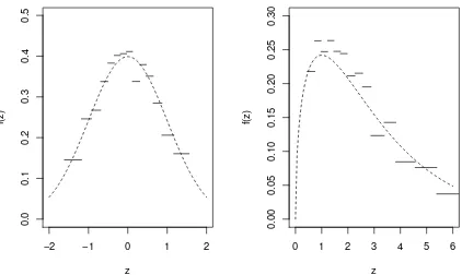
To further illustrate how the LID method operates, we randomly generated two data sets of size n = 1000, one from the standard normal distribution and the other from χ2 _{distribution with} _df _{= 3. Figure 2.1 shows that the LID well describes the overall}

(30)

spaced quantile levels from 0.0625 to 0.9375 were used. The dashed curves depict the true densities and the solid lines correspond to the approximate density estimates by the LID method. The approximate densities are piecewise constant functions and inversely proportional to the distance between two adjacent sample quantiles.

−2 −1 0 1 2

0.0

0.1

0.2

0.3

0.4

0.5

z

f(z)

0 1 2 3 4 5 6

0.00

0.05

0.10

0.15

0.20

0.25

0.30

z

f(z)

Figure 2.1: The LID estimates for data sets generated fromN(0,1) andχ2

3. The dashed

curves are the true density functions and the solid lines are the LID estimations toN(0,1) (the left plot) and χ2

3 (the right plot) .

The LID method can be applied to estimate the density of z at any point that lies between the τ1 and τK-th quantiles. However, it is difficult to use the LID method for

(31)

and its limitations in Section 2.3 under the regression setup.

2.2 LID Method for Linear Quantile Regression

2.2.1 Benefits of the LID method

Most existing Bayesian methods focus on a single quantile level and those approaches may encounter quantile crossing problem and inconsistency of likelihood when the analysis is carried out at multiple quantile levels.

In contrast, the LID method avoids those limitations by joint-modeling of multiple quantiles under the assumption that the quantiles of the response are linear in covariates. With this joint-modeling, we can avoid quantile crossing and achieve higher efficiency of estimating quantile coefficients. The method will be discussed in Section 2.2.2 and the efficiency will be assessed via simulation studies in Section 2.4.

2.2.2 LID for Linear Quantile Regression

We introduce the LID method of Feng (2011) for Bayesian quantile regression. Let’s consider the linear quantile regression model,

Qτ(Y|X) =XTβτ, 0< τ <1, (2.2) whereY is the response,Xis ap-dimensional covariate vector andβ_τ is thep-dimensional vector of quantile coefficients. Suppose that we observe a random sample, (y,x) = {(yi,xi), i= 1, ...n}of (Y,X), and we are interested in estimatingβK = (β

T

τ1,· · · ,β

T τk)

T_, where 0< τ1 <· · ·< τK <1 is a sequence of quantile levels.

By the Bayes rule, the posterior distribution of β_K given (y,x) is

f(β_K|y,x)∝ n Y i=1

fY(yi|xi,βK)π(βK), (2.3)

where π(β_K) denotes the prior distribution of β_K.

(32)

quantile functions atτk,k = 1,· · · , K.Using the idea of the integrated likelihood methods by Berger et al. (1999), the conditional density fY(yi|xi,βK) is defined by

fY(yi|xi,βK) = Z

fj(yi|xi)π(fj|xi,βK)dfj,

where fj(y|xi) is the conditional density function of Y given X = xi that leads to the same conditional quantile functions atτk, k= 1,· · · , K and π(fj|xi,β_K) is the prior on fj(Yi|xi). Then, we can interpret fY(yi|xi,βK) as the approximate likelihood averaged over all possible fj’s that share the same conditional quantiles at the K quantile levels.

Note that we can link the conditional density function fY(·|x,βK) with model (2.2) by the following equation:

fY(y|x,βK) = lim δ→0

δ

xT₍_β

uy+δ−βuy)

,

where uy = {τ ∈ (0,1) : xTβτ = y}. Let 0 < τ1 < · · · < τK < 1 be a grid of quantile levels. Therefore, for any y with associated covariate x such that F_Y−1(τj|x,βK) < y < F_Y−1(τj+1|x,βK) for some j = 1, . . . , K −1, we can approximate fY(y|x,βK) by

τj+1−τj

xT₍_β

τj+1−βτj)

.

Feng (2011) proposed a Bayesian quantile regression procedure based on the following linearly interpolated density (LID)

ˆ

fY(yi|xi,β_K) =I{yi ∈(−∞,xT_i β_τ₁)}τ1f1(yi)

+ K−1

X k=1

I{yi ∈[xTi βτk,x

T

i βτk+1)}

τk+1−τk

xT

i βτk+1 −x

T i βτk

+I{yi ∈[xTi βτK,∞)}(1−τK)f2(yi), i= 1, . . . , n, (2.4)

where f1 and f2 are some prespecified left and right tail density functions.

Particu-larly, Feng (2011) assumed f1(·) and f2(·) to be the truncated normal distributions

N₍−∞,xT iβτ₁](x

T i βτ1, σ

2

1) andN(xT

iβτk,∞)(x

T i βτk, σ

2

2), respectively, whereσ1 andσ2 are some

pre-specified scale parameters. The LID method may be senesitive to the seletion of σ2. Hence, in the simulation studies, we consider several values for σ2

(33)

we can avoid pre-specifying σ2

1 and σ22 by matching the linearly interpolated density and

truncated normal tail density atxT

iβτ1 andx

T

i βτk, that is, we can estimateσ

2

1 andσ22 by

ˆ

σ1 = 2τ1

n X

i=1

xT

i βτ2 −x

T i β(τ1)

n√2π(τ2−τ1)

and

ˆ

σ2 = 2{1−τK) n X

i=1

xT

i βτk −x

T i βτK−1

n√2π(τK−τK−1)

.

Algorithm of LID for Linear Quantile Regression

We describe the algorithm for drawing samples from the approximate posterior distribu-tions. Given the approximate likelihood ˆfY(yi|xi,βK) and the priorπ(βK), we draw the posterior samples of β_K using the following algorithm.

Step 1. Choose initial values for the quantile coefficients β(0)_K .

(a) Apply the conventional quantile regression. First, regress yi on xi at each quantile level τk, k = 1, ..., K, separately and obtain β

(0)

K . We can use the rq function in the R package “quantreg.”

Step 2. Propose a move.

(a) Randomly pick a quantile level, τk, and select a random number from 1 to p, say l. Then, let β_l,τ∗

k denote the candidate forβl,τk, the lth element of βτk.

(b) To avoid quantile crossing, we draw β_l,τ∗

k from a proposal distribution that

satisfies the following monotonicity constraints for all i= 1,· · · , n:

xT_i β_τ

K−1 ≤x

T

i βτk, k= 2, ..., K.

The further description of the proposal distribution is given in the Appendix. The l-th element of β_τ

k will be replaced by β

∗

l,τk, generating the candidateβ

∗

K. Step 3. Take

β(_Kt+1) = (

β∗_K with probability φ(β(_Kt),β∗_K)

(34)

where

φ(β(_Kt),β∗_K) = min (_Qn

i=1fˆY(yi|xi,β

∗

K)π(β

∗

K) Qn

i=1fˆY(yi|xi,β

(t)

K)π(β

(t)

K) ,1

) ,

where π(·) is the prior of β_K and ˆfY(y|x,βK) is the approximate density as in (2.4).

Step 4. Repeat Steps 2 and 3 until the MCMC chain converges. After a burn-in period, we obtain posterior samples of β_K. We estimate each parameter by using the mean of the samples.

2.3 LID Method with Improved Tail Density

Esti-mation

The method of Feng (2011) relies on the specification of the tail densitiesf1 and f2 and

the scale parameter σ. Our numerical studies suggest that the method could be sensitive to the choice of σ; see Section 2.4. Moreover, truncated normal distributions might not work well for estimating tails of asymmetric, skewed or heavy-tailed error distributions. To improve the tail estimation, we propose a modified approximate likelihood, which estimates the tail densities based on extreme value theory and does not require any prespecification of parameters.

Pickands (1975) and Balkema and de Haan (1974) showed that if the distribution function F of a random variable Y belongs to the domain of attraction of generalized extreme value distribution, then as u→yF, the end point ofF, the conditional distribu-tion funcdistribu-tion P(Y ≤u+y|Y > u) approaches the distribution function of a generalized Pareto distribution (GPD). That is, as u→yF,

P(Y ≤u+y|Y > u)→G(y|%, ξ) = (

1−(1 +ξy/%)−1/ξ, ξ6= 0 1−exp(−y/%), ξ = 0,

wherey >0 forξ ≥0 and 0≤y <−%/ξ forξ <0 with ξ and % >0 being the shape and scale parameters of the GPD, respectively.

(35)

Y by linear interpolation of conditional quantiles at the central quantiles while use the GPD to approximate the tail densities.

For right tails, we define the upper thresholds ui = {xTi βτK +x

T

i βτK−1}/2 and

ap-proximate the tail distribution by the generalized Pareto distribution (GPD) with scale parameter %2 >0 and shape parameter ξ2, G(y|%2, ξ2), that is,

P(Y < y|y > ui,xi)≈G(y−ui|%2, ξ2).

Note that

P(Y < y|y > ui,xi) =

P(Y < y|xi)−P(Y < ui|xi) P(Y > ui|xi)

≈ F(y|xi)−(τK+τK−1)/2 1−(τK +τK−1)/2

.

Therefore, the right tail density for y >xT_i β_τ_K can be approximated by ˆ

fY(y|xi,βK) = (1−τK)f2(y|xi,βK, %2, ξ2)≈ {1−(τK−1+τK)/2}g(y−ui|%2, ξ2),

(2.5) where g(·, %, ξ) is the density function of GPD(%, ξ) defined as

g(y|%, ξ) = (

%−1_{(1 +}_ξy/%)−(1+1/ξ)_, _ξ_{6= 0}

%−1_exp(−y/%), _ξ _{= 0,}

with y >0 forξ ≥0 and 0≤y <−%/ξ for ξ <0.

The scale parameter%in the GPD can be estimated by matching the LID ˆfY(y|xi,βK) and g(y−ui|%r, ξr) at y=ui. Specifically, for ui =xTi (βτK +βτK−1)/2, note that

ˆ

fY(ui|xi,βK)≈ {1−(τK−1+τK)/2)}g(0|%2, ξ2)

⇔ τK−τK−1

xT

i (βτK −βτK−1)

≈ {1−(τK−1+τK)/2)} 1 %2

.

Then, the scale parameter %2 can be estimated by

ˆ

%2 ={1−(τK−1+τK)/2)} n X

i=1

xT_i ( ˜β_τ_K −β˜_τ_K₋₁) n(τK−τK−1)

, (2.6)

where ˜β_τ

(36)

choose ˜β_τ

k as the conventional (frequentist) quantile regression estimator defined as

˜

β_τ

k = arg min_β

n X

i=1

ρτk(yi−x

T i β),

with ρτ(u) =u{τ −I(u <0)}being the quantile loss function; see Koenker and Bassett (1978). The estimator ˜β_τ_k is obtained by applying the “rq” function in the R package

quantreg at theτkth quantile.

Note that if we define W = −Y, then Qτ(W|x) = −Q1−τ(Y|x), that is, the lower tail of Y corresponds to the upper tail of W. Define the lower thresholds li ={xTi βτ1 +

xT

i βτ2}/2. For y <x

T

i βτ1, the left tail density can be approximated by

ˆ

fY(y|xi,βK) =τ1f1(y|xi,βK, %1, ξ1)≈g(−y+li|%1, ξ1)(τ1 +τ2)/2, (2.7)

where %1 >0 is the scale parameter andξ1 is the shape parameter.

Similarly, by matching the GPD density with LID aty=li, we can estimate the scale parameter %1 by

ˆ

%1 = (τ1+τ2)/2

n X

i=1

xT

i β˜τ2 −x

T i β˜τ1

n(τ2−τ1)

. (2.8)

The shape parametersξ1andξ2 can then be estimated by maximizing the GPD likelihood

based on the exceedances {yi : yi < li, i = 1, . . . , n} and {yi : yi > ui, i = 1, . . . , n}, respectively.

In our implementation, we first estimate the shape and scale parameters %1, %2, ξ1,

ξ2 based on the initial estimator ˜βK = ( ˜β T τ1, . . . ,

˜

βT_τ

K)

T_{, and then keep them unchanged} throughout the Markov chain Monte Carlo (MCMC) simulations. Alternatively, we could also update the shape and scale parameters in the MCMC. However, our numerical studies show that the latter approach complicates the algorithm without improving the performance.

The algorithm of the proposed LID method with GPD tail approximation requires an additional procedure in Step 1.

Step 1. Choose initial values for the quantile coefficients β(0)_K .

(37)

quantile level τk, k = 1, ..., K, separately and obtain β

(0)

K . We can use the rq function in the R package “quantreg.”

(b) Obtain the scale parameter estimates, ˆ%1 and ˆ%2 from the equations (2.8) and

(2.6), respectively, using the initial β(0)_K . Then, obtain the shape parameter estimates, ˆξ1 and ˆξ2, by using the f itgpd function in the R package “POT.”

1.0 1.5 2.0 2.5

0.0

0.1

0.2

0.3

0.4

0.5

n=100

z

f(z)

True density

GPD tail approximation

1.0 1.5 2.0 2.5

0.0

0.1

0.2

0.3

0.4

0.5

1.0 1.5 2.0 2.5

0.0

0.1

0.2

0.3

0.4

0.5

n=200

z

f(z)

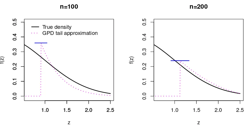
Figure 2.2: The estimated upper tail densities for random samples of size 100 and 200 from the standard normal distribution. The horizontal axis represents z and the vertical axis represents the density. The dotted vertical lines arez = ˆΦ−1_{(0.85). The solid curves}

are the true density and the dotted curves correspond to the GPD tail approximation.

Figure 2.2 illustrates right-tail density approximations using the proposed method for random samples of size 100 and 200 from the standard normal distribution. The shape and scale parameters are estimated using exceedances over the 85-th percentile of each random sample. We can observe that the GPD tail approximations are getting finer with larger sample size.

(38)

the constraints in the proposal distributions. Appendix A.2 summarizes different versions of LIGPD and LID. These versions lead to more complicated algorithms without much improvement in the performance. Hence, our proposed LIGPD method first estimate the shape and scale parameters based on the initial estimator and then keep them unchanged throughout the MCMC simulations.

2.4 Simulation Studies

We carry out two simulation studies to compare the performance of the LID method (Feng, 2011), the proposed LIGPD method, and the conventional frequentist quantile regression method (Koenker and Bassett, 1978).

2.4.1 Simulation Study I

We consider the following model for generating the simulation data:

yi =β0+β1xi+ (1 +xi)i, i= 1, . . . , n, (2.9) where xi ∼ LN(0,1), (β0, β1) = (2,4) and LN(µ, ς) is the log normal distribution with

location parameter µand scale parameterς. We consider three distributions for generat-ing the random errors: the standard normal, t3, and χ21. The corresponding conditional

quantile function is

Qτ(Y|xi) = β0,τ +β1,τxi,

where β0,τ = 2 +F−1(τ),β1,τ = 4 +F−1(τ) and F is the distribution function ofi. For each scenario, the simulation is repeated 200 times. In the following, we refer to the conventional quantile regression method as QR, the LID method proposed by Feng (2011) based on truncated normal tail distributions with pre-specified variance parameters as LID, the LID method with the proposed variance parameter selection method suggested in Section 2.2.2 as LID II and the proposed method that approximates the tail density using GPD as LIGPD.

We generate n = 100,200 and 500 observations from model (2.9). For both LID and LIGID methods, we use a grid of K = 7,11 and 15 equally spaced quantile levels τk=k/(1 +K), k = 1,· · · , K, and assign the normal priors N(0,Σ) to (βτ1,· · · ,βτK)

T_, where β_τ_k = (β0,τk, β1,τk)

(39)

we discard the first 50,000 as burn-in, and estimate βj,τ for j = 0,1 by the posterior means of the thinned sample using every 100th draw of the MCMC chain. Following the suggestions in Feng et al. (2014), for the LID method, we take the left tail density f1(·) as the left half of N(xTi βτ1, σ

2_{) and the right tail density} _f

2(·) as the right half

of N(xT i βτK, σ

2_{) with} _x

i = (1, xi)T and σ2 a pre-specified constant. To examine the dependence of LID on the choice of σ, we consider σ = 0.5,1,1.5,2 and 3 for both the normal and t3 error distributions and σ1 = 0.5 and σ2 = 1,2,3,4,5 forχ21 errors.

The posterior means were used as the estimates for βj.τ, j = 0,1, τ = 0.25,0.5,0.75. The mean squared errors (MSE) were obtained by

1 200

200

X m=1

{βˆ_j,τ(m)−βj,τ}2, (2.10)

where ˆβ_j,τ(m), j = 0,1 are the candidate estimators for the intercept and slope in them-th simulation run.

Mean Squared Error Comparison

Tables 2.1–2.3 summarize the mean squared errors of coefficient estimates from different methods at three quartiles (τ=0.25, 0.5, 0.75) for the standard normal, t3 and χ21

distri-butions, respectively. The results for the LID estimator in Tables 2.1–2.3 are based on “optimal”σ that give us the smallest sums of the mean squared errors ofβ0,τ and β1,τ at τ = 0.25,0.5,0.75, β0,.75−β0,.5 and β1,.75−β1,.5. Figures 2.3–2.5 show the mean squared

errors ofβ0,τ and β1,τ atτ = 0.25,0.5,0.75, β0,.75−β0,.5 and β1,.75−β1,.5 for QR and LID,

LID II and LIGPD with K = 7 and the ranges of the mean squared errors for LID. For normal errors, the LID, LID II and LIGPD estimators show comparable or higher efficiency than the QR estimator for all three sample sizes. One possible explanation is that the QR method fits quantile regression at each quantile level separately without making any distributional assumptions or attempting to model the distribution, while the LID, LID II and LIGPD aim to estimate the conditional distribution of Y by using the additional assumption of global linearity of quantile functions.

Fort3errors, the LID, LID II and LIGPD estimators withK = 7 show higher efficiency

(40)

approximation, the LIGPD method does not have clear efficiency gain over the LID with the “optimal” σ for small samples sizes. The LIGPD estimator has some efficiency gain over the LID II estimator.

For χ2

1 random errors, the LID, LID II and LIGPD estimators show higher efficiency

than the QR estimator for n = 100 and 200. The LID method with the “optimal” σ was the most efficient for n= 100 and 200 but the LID II and LIGPD show comparable results for all sample sizes. Forn = 500, all three estimators have similar efficiency when K = 7. For K = 15 andn= 100, the LIGPD estimator shows higher MSEs than the QR and LID estimators because small sample size makes poor estimation of tail probability. Tables 2.1–2.3 show that the LIGPD and LID estimators have comparable or higher efficiency than the QR estimator, especially for moderate sample sizen = 100 and 200. In general, results suggest that, by using GPD approximation, the LIGPD leads to similar or more efficient estimation than the LID based on the “optimal” σ for N(0,1) and t3

errors and than the LID II estimator for all error distributions. The efficiency gain of LIGPD over LID is not obvious in small sample sizes, since the GPD approximation to tail density does not work well for small sample sizes.

To examine the sensitivity of the LID method to the choice ofσ, we plot the MSEs of the QR and LIGPD estimators and the ranges of MSEs of the LID estimators based on different choices ofσ in Figures 2.3–2.5. These figures suggest that not-well selectedσ in the LID estimator may result in high MSE and that the LID method is very sensitive to the choice ofσin all scenarios considered. Ifσis chosen inappropriately, the performance of LID could be much worse than LIGPD and even worse than the regular QR method in some cases. Note that in our implementation of the LID, we chooseσ involved inf1 and

f2 among few choices that gives LID estimates with the smallest mean squared errors.

This option is in favor of the LID method. However, in practice this choice is not feasible.

Quantile Crossing Issue

(41)

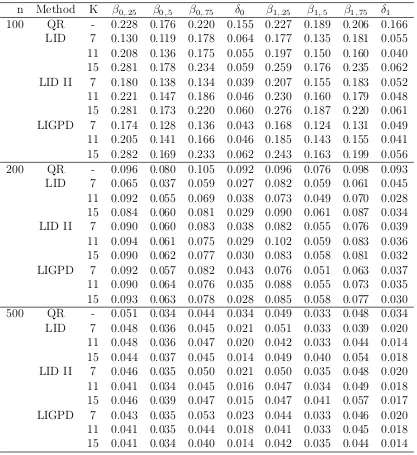
Table 2.1: Mean squared errors of parameter estimators for data generated from model (2.9) with i ∼N(0,1) from the conventional quantile regression method (QR), the LID method of Feng (LID) based on the “optimal” σ, the LID method with the proposed variance parameter selection method (LID II) and the proposed LIGPD method using GPD tail density approximation (LIGPD), whereδ0=β0,.75−β0,.5 and δ1=β1,.75−β1,.5.

n Method K β0,.25 β0,.5 β0,.75 δ0 β1,.25 β1,.5 β1,.75 δ1

(42)

Table 2.2: Mean squared errors of parameter estimators for data generated from model (2.9) with i ∼ t3 from the conventional quantile regression method (QR), the LID

method of Feng (LID) based on the “optimal” σ, the LID method with the proposed variance parameter selection method (LID II) and the proposed LIGPD method using GPD tail density approximation (LIGPD), whereδ0=β0,.75−β0,.5 and δ1=β1,.75−β1,.5.

(43)

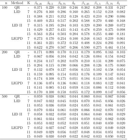
Table 2.3: Mean squared errors of parameter estimators for data generated from model (2.9) with i ∼ χ21 from the conventional quantile regression method (QR), the LID

method of Feng (LID) based on the “optimal” σ, the LID method with the proposed variance parameter selection method (LID II) and the proposed LIGPD method using GPD tail density approximation (LIGPD), whereδ0=β0,.75−β0,.5 and δ1=β1,.75−β1,.5.

(44)