Sustained Space Complexity
Jo¨el Alwen1,3, Jeremiah Blocki2, and Krzysztof Pietrzak1 1
IST Austria
2
Purdue University
3
Wickr Inc.
Abstract. Memory-hard functions (MHF) are functions whose eval-uation cost is dominated by memory cost. MHFs are egalitarian, in the sense that evaluating them on dedicated hardware (like FPGAs or ASICs) is not much cheaper than on off-the-shelf hardware (like x86 CPUs). MHFs have interesting cryptographic applications, most notably to password hashing and securing blockchains.
Alwen and Serbinenko [STOC’15] define the cumulative memory com-plexity (cmc) of a function as the sum (over all time-steps) of the amount of memory required to compute the function. They advocate that a good MHF must have high cmc. Unlike previous notions, cmc takes into ac-count that dedicated hardware might exploit amortization and paral-lelism. Still, cmc has been critizised as insufficient, as it fails to capture possible time-memory trade-offs; as memory cost doesn’t scale linearly, functions with the same cmc could still have very different actual hard-ware cost.
In this work we address this problem, and introduce the notion of sustained-memory complexity, which requires that any algorithm evaluating the function must use a large amount of memory for many steps. We con-struct functions (in the parallel random oracle model) whose sustained-memory complexity is almost optimal: our function can be evaluated usingnsteps andO(n/log(n)) memory, in each step making one query to the (fixed-input length) random oracle, while any algorithm that can make arbitrary many parallel queries to the random oracle, still needs
Ω(n/log(n)) memory forΩ(n) steps.
As has been done for various notions (including cmc) before, we reduce the task of constructing an MHFs with high sustained-memory com-plexity to proving pebbling lower bounds on DAGs. Our main technical contribution is the construction is a family of DAGs on n nodes with constant indegree with high “sustained-space complexity”, meaning that any parallel black-pebbling strategy requiresΩ(n/log(n)) pebbles for at leastΩ(n) steps.
Along the way we construct a family of maximally “depth-robust” DAGs with maximum indegree O(logn), improving upon the construction of
Mahmoody et al. [ITCS’13] which had maximum indegreeO log2n·polylog(logn).
1
Introduction
asymmetry in the capabilities of honest and dishonest parties. An example are trapdoor functions, where the honest party – who knows the secret trapdoor key – can efficiently invert the function, whereas a potential adversary – who does not have this key – cannot.
1.1 Moderately-Hard Functions
Moderately hard functions consider a setting where there’s no asymmetry, or even worse, the adversary has more capabilities than the honest party. What we want is that the honest party can evaluate the function with some reason-able amount of resources, whereas the adversary should not be reason-able to evaluate the function at significantly lower cost. Moderately hard functions have several interesting cryptographic applications, including securing blockchain protocols and for password hashing.
An early proposal for password hashing is the “Password Based Key Deriva-tion FuncDeriva-tion 2” (PBKDF2) [Kal00]. This function just iterates a cryptographic hash function like SHA1 several times (1024 is a typical value). Unfortunately,
PBKDF2doesn’t make for a good moderately hard function, as evaluating a cryp-tographic hash function on dedicated hardware like ASCIs (Application Specific Integrated Circuits) can be by several orders of magnitude cheaper in terms of hardware and energy cost than evaluating it on a standard x86 CPU. An economic analysis of Blocki et al. [BHZ18] suggests that an attacker will crack
almost allpasswords protected byPBKDF2. There have been several suggestions how to construct better, i.e., more “egalitarian”, moderately hard functions. We discuss the most prominent suggestions below.
Memory-Bound Functions Abadi et al. [ABW03] observe that the time required to evaluate a function is dominated by the number of cache-misses, and these slow down the computation by about the same time over different architectures. They proposememory-boundfunctions, which are functions that will incur many expensive cache-misses (assuming the cache is not too big). They propose a construction which is not very practical as it requires a fairly large (larger than the cache size) incompressible string as input. Their function is then basically pointer jumping on this string. In subsequent work [DGN03] it was shown that this string can also be locally generated from a short seed.
Memory-Hard Functions Whereas memory-bound and bandwidth-hard tions aim at being egalitarian in terms of time and energy, memory-hard func-tions (MHF), proposed by Percival [Per09], aim at being egalitarian in terms of hardware cost. A memory-hard function, in his definition, is one where the memory used by the algorithm, multiplied by the amount of time, is high, i.e., it has high space-time (ST) complexity. Moreover, parallelism should not help to evaluate this function at significantly lower cost by this measure. The rationale here is that the hardware cost for evaluating an MHF is dominated by the mem-ory cost, and as memmem-ory cost does not vary much over different architectures, the hardware cost for evaluating MHFs is not much lower on ASICs than on standard CPUs.
Cumulative Memory Complexity Alwen and Serbinenko [AS15] observe that ST complexity misses a crucial point, amortization. A function might have high ST complexity because at some point during the evaluation the space requirement is high, but for most of the time a small memory is sufficient. As a consequence, ST complexity is not multiplicative: a function can have ST complexityC, but evaluating X instances of the function can be done with ST complexity much less than X ·C, so the amortized ST cost is much less than C. Alwen and Blocki [AB16,AB17] later showed that prominent MHF candidates such as Ar-gon2i [BDK16], winner of the Password Hashing Competition [PHC] do not have high amortized ST complexity.
To address this issue, [AS15] put forward the notion of cumulative-memory complexity (cmc). The cmc of a function is the sum – over all time steps – of the memory required to compute the function by any algorithm. Unlike ST complexity, cmc is multiplicative.
Sustained-Memory Complexity Although cmc takes into account amortization and parallelism, it has been observed (e.g., [RD16,Cox16]) that it still is not suf-ficient to guarantee egalitarian hardware cost. The reason is simple: if a function has cmcC, this could mean that the algorithm minimizing cmc uses someT time steps andC/T memory on average, but it could also mean it uses time 100·T andC/100·T memory on average. In practice this can makes a huge difference becausememory cost doesn’t scale linearly. The length of the wiring required to access memory of sizeM grows like√M (assuming a two dimensional layout of the circuit). This means for one thing, that – as we increaseM – the latency of accessing the memory will grow as√M, and moreover the space for the wiring required to access the memory will grow likeM1.5.
The exact behaviour of the hardware cost as the memory grows is not crucial here, just the point that it’s superlinear, and cmc does not take this into account. In this work we introduce the notion of sustained-memory complexity, which takes this into account. Ideally, we want a function which can be evaluated by a “na¨ıve” sequential algorithm (the one used by the honest parties) in time T using a memory of sizeS where (1) S should be close toT and (2) anyparallel
Property (1) is required so the memory cost dominates the evaluation cost already for small values ofT. Property (2) means that even a parallel algorithm will not be able to evaluate the function at much lower cost; any parallel algo-rithm must make almost as many steps as the na¨ıve algoalgo-rithm during which the required memory is almost as large as the maximum memorySused by the na¨ıve algorithm. So, the cost of the best parallel algorithm is similar to the cost of the na¨ıve sequential one, even if we don’t charge the parallel algorithm anything for all the steps where the memory is belowS0.
Ren and Devadas [RD16] previously proposed the notion of “consistent mem-ory hardness” which requires that any sequentialevaluation algorithm must ei-ther use space S0 for at least T0 steps, or the algorithm must run for a long time e.g.,T n2. Our notion of sustained-memory complexity strengthens this notion in that we considerparallelevaluation algorithms, and our guarantees are absolute e.g., even if a parallel attacker runs for a very long time he must still use memoryS0 for at leastT0steps.scrypt[Per09] is a good example of a MHF that has maximal cmcΩ n2
[ACP+17] that does not have high sustained space complexity. In particular, forany memory parameterM and any running time parameternwe can evaluatescrypt[Per09] in timen2/M and with maximum spaceM. As was argued in [RD16] an adversary may be able to fitM =n/100 space in an ASIC, which would allow the attacker to speed up computation by a factor of more than 100 and may explain the availability of ASICs forscrypt
despite its maximal cmc.
In this work we show that functions with asymptotically optimal sustained-memory complexity exist in the random oracle model. We note that we must make some idealized assumption on our building block, like being a random oracle, as with the current state of complexity theory, we cannot even prove superlinear circuit lower-bounds for problems in N P. For a given time T, our function uses maximal space S ∈ Ω(T) for the na¨ıve algorithm,4 while any
parallel algorithm must have at least T0 ∈ Ω(T) steps during which it uses memoryS0∈Ω(T /log(T)).
Graph Labelling The functions we construct are defined by directed acyclic graphs (DAG). For a DAGGn= (V, E), we order the verticesV ={v1, . . . , vn} in some topological order (so if there’s a path fromi to j then i < j), withv1 being the unique source, and vn the unique sink of the graph. The function is now defined by Gn and the input specifies a random oracle H. The output is the label `n of the sink, where the label of a node vi is recursively defined as `i=H(i, `p1, . . . , `pd) wherevp1, . . . , vpd are the parents ofvi.
Pebbling Like many previous works, including [ABW03,RD17,AS15] discussed above, we reduce the task of proving lower bounds – in our case, on sustained memory complexity – for functions as just described, to proving lower bounds on some complexity of a pebbling game played on the underlying graph.
4
For example, Ren and Devedas [RD17] define a cost function for the so called reb-blue pebbling game, which then implies lower bounds on the bandwidth hardness of the function defined over the corresponding DAG.
Most closely related to this work is [AS15], who show that a lower bound the so called sequential (or parallel)cumulative (black) pebbling complexity (cpc) of a DAG implies a lower bound on the sequential (or parallel) cumulative memory complexity (cmc) of the labelling function defined over this graph. Alwen et al. [ABP17] constructed a constant indegree family of DAGs with parallel cpc Ω(n2/log(n)), which is optimal [AB16], and thus gives functions with optimal cmc. More recently, Alwen et al. [ABH17] extended these ideas to give the first
practicalconstruction of an iMHF with parallel cmcΩ(n2/log(n)).
The black pebbling game – as considered in cpc – goes back to [HP70,Coo73]. It is defined over a DAGG= (V, E) and goes in round as follows. Initially all nodes are empty. In every round, the player can put a pebble on a node if all its parents contain pebbles (arbitrary many pebbles per round in the parallel game, just one in the sequential). Pebbles can be removed at any time. The game ends when a pebble is put on the sink. The cpc of such a game is the sum, over all time steps, of the pebbles placed on the graph. The sequential (or parallel) cpc ofGis the cpc of the sequential (or parallel) black pebbling strategy which minimizes this cost.
It’s not hard to see that the sequential/parallel cpc ofGdirectly implies the same upper bound on the sequential/parallel cmc of the graph labelling function, as to compute the function in the sequential/parallel random oracle model, one simply mimics the pebbling game, where putting a pebble on vertex vi with parentsvp1, . . . , vpd corresponds to the query`i←H(i, `p1, . . . , `pd). And where one keeps a label`jin memory, as long asvj is pebbled. If the labels`i ∈ {0,1}w arewbits long, a cpc ofptranslates to cmc ofp·w.
More interestingly, the same has been shown to hold for interesting notions also for lower bounds. In particular, the ex-post facto argument [AS15] shows that any adversary who computes the label `n with high probability (over the choice of the random oracleH) with cmc ofm, translates into a black pebbling strategy of the underlying graph with cpc almostm/w.
In this work we define the sustained-space complexity (ssc) of a sequen-tial/parallel black pebbling game, and show that lower bounds on ssc translate to lower bounds on the sustained-memory complexity (smc) of the graph labelling function in the sequential/parallel random oracle model.
Thus, to construct a function with high parallel smc, it suffices to construct a family of DAGs with constant indegree and high parallel ssc. In Section 3 we construct such a family {Gn}n∈N of DAGs where Gn has n vertices and has indegree 2, whereΩ(n/log(n))-ssc is inΩ(n). This is basically the best we can hope for, as our bound on ssc trivially implies a Ω(n2/log(n)) bound on csc, which is optimal for any constant indegree graph [AS15].
Data-Dependent vs Data-Independent MHFs There are two categories of Mem-ory Hard Functions: data-Independent MemMem-ory Hard Functions (iMHFs) and data-dependent Memory Hard Functions (dMHFs). As the name suggests, the algorithm to compute an iMHFs must induce a memory access pattern that is
independentof the potentially sensitive input (e.g., a password), while dMHFs have no such constraint. While dMHFs (e.g., scrypt [PJ12], Argon2d, Ar-gon2id [BDK16]) are potentially easier to construct, iMHFs (e.g., Argon2i [BDK16], DRSample [ABH17]) are resistant to side channel leakage attacks such as cache-timing. For the cumulative memory complexity metric there is a clear gap be-tween iMHFs and dMHFs. In particular, it is known that scrypt has cmc at
leastΩ n2w
[ACP+17], whileanyiMHF has cmcat mostOn2wlog logn logn
.
In-terestingly, the same gap doesnothold for smc. In particular, any dMHF can be computed withmaximum space O(nw/logn+nlogn) by recursively applying a result of Hopcroft et al. [HPV77]5.
1.2 High Level Description of our Construction and Proof
Our construction of a family{Gn}n∈N of DAGs with optimal ssc involves three
building blocks:
The first building block is a construction of Paul et al. [PTC76] of a family of DAGs{PTCn}n∈N withindeg(PTCn) = 2 and space complexityΩ(n/logn). More significantly for us they proved that for any sequential pebbling ofGnthere is a time interval [i, j] during which at leastΩ(n/logn) new pebbles are placed on sources of Gn and at least Ω(n/logn) are always on the DAG. We extend the proof of Paul et al. [PTC76] to show that the same holds for any parallel
pebbling of PTCn; a pebbling game first introduced in [AS15] which natural 5 To see this let G denote the data-dependency DAG that will be produced as we
evaluate the dMHF. Initially, some of the edges in the graph are unknown, but we can allocate spacenlognto keep track of the edges as they are dynamically generated during computation. Hopcroft et al. [HPV77] showed that any static DAG G on
models parallel computation. We can argue that j−i = Ω(n/logn) for any sequential pebbling since it takes at least this many steps to placeΩ(n/logn) new pebbles on Gn. However, we stress that this argument does not apply to parallel pebblings so this does not directly imply anything about sustained space complexity for parallel pebblings.
To address this issue we introduce our second building block: a family of {D
n}n∈N of extremely depth robust DAGs with indeg(Dn) ∈ O(logn) — for
any constant >0 the DAGD
n is (e, d)-depth robust for anye+d≤(1−)n. We remark that our result improves upon the construction of Mahmoody et al. [MMV13] whose construction required indeg(Dn)∈O log2npolylog(logn)
and may be of independent interest (e.g., our construction immediately yields a more efficient construction of proofs of sequential work [MMV13]). Our con-struction ofDn is (essentially) the same as Erdos et al. [EGS75] albeit with much tighter analysis. By overlaying an extremely depth-robust DAG Dn on top of the sources of PTCn, the construction of Paul et al. [PTC76], we can ensure that it takes Ω(n/logn) steps to pebble Ω(n/logn) sources of Gn. However, the resulting graph would haveindeg(Gn)∈O(logn) and would have sustained spaceΩ(n/logn) for at mostO(n/logn) steps. By contrast, we want a n-node DAG Gwith indeg(G) = 2 which requires space Ω(n/logn) for at least Ω(n) steps6.
Our final tool is to apply the indegree reduction lemma of Alwen et al. [ABP17] to{D
t}t∈Nto obtain a family of DAGs{J
t}t∈Nsuch thatJ
t hasindeg(Jt) = 2 and 2t·indeg(D
t)∈O(tlogt) nodes. Each node inDt is associated with a path of length 2·indeg(D
t) inJt and each pathpin Dt corresponds to a path p0 of length|p0| ≥ |p| ·indeg(Gt) inJ
t. We can then overlay the DAGJt on top of the sources inPTCn where t=Ω(n/logn) is the number of sources inPTCn. The final DAG has sizeO(n) and we can then show that any legal parallel pebbling requiresΩ(n) steps with at leastΩ(n/logn) pebbles on the DAG.
2
Preliminaries
In this section we introduce common notation, definitions and results from other work which we will be using. In particular the following borrows heav-ily from [ABP17,AT17].
6
We typically want a DAGGwithindeg(G) = 2 because the compression functionH
which is used to label the graph typically maps 2wbit inputs towbit outputs. In this case the labeling function would only be valid for graphs with maximum indegree two. If we used tricks such as Merkle-Damgard to build a new compression functionG
2.1 Notation
We start with some common notation. Let N ={0,1,2, . . .}, N+ ={1,2, . . .},
and N≥c ={c, c+ 1, c+ 2, . . .} for c ∈N. Further, we write [c] := {1,2, . . . , c}
and [b, c] ={b, b+ 1, . . . , c} wherec≥b∈N. We denote the cardinality of a set
B by|B|.
2.2 Graphs
The central object of interest in this work are directed acyclic graphs (DAGs). A DAGG= (V, E) hassizen=|V|. The indegree of nodev∈V isδ=indeg(v) if there existδincoming edgesδ=|(V × {v})∩E|. More generally, we say that Ghas indegreeδ=indeg(G) if the maximum indegree of any node ofGisδ. If
indeg(v) = 0 thenv is called asource node and ifv has no outgoing edges it is called asink. We useparentsG(v) ={u∈V : (u, v)∈E}to denote the parents of a nodev∈V. In general, we useancestorsG(v) :=Si≥1parentsiG(v) to denote the set of all ancestors of v — here, parents2
G(v) :=parentsG(parentsG(v)) denotes the grandparents of v and parentsi+1G (v) := parentsG parentsi
G(v)
. When G is clear from context we will simply write parents (ancestors). We denote the set of all sinks of G with sinks(G) = {v ∈ V : @(v, u) ∈ E} — note that
ancestors(sinks(G)) =V. The length of a directed pathp= (v1, v2, . . . , vz) inG is the number of nodes it traverseslength(p) := z. The depthd =depth(G) of DAGGis the length of the longest directed path inG. We often consider the set of all DAGs of fixed sizenGn:={G= (V, E) : |V|=n}and the subset of those DAGs at most some fixed indegree Gn,δ :={G ∈Gn : indeg(G) ≤δ}. Finally, we denote the graph obtained fromG= (V, E) by removing nodesS ⊆V (and incident edges) byG−Sand we denote byG[S] =G−(V\S) the graph obtained by removing nodesV \S (and incident edges).
The following is an important combinatorial property of a DAG for this work.
Definition 1 (Depth-Robustness). For n ∈ N and e, d ∈ [n] a DAG G =
(V, E)is(e, d)-depth-robust if
∀S⊂V |S| ≤e⇒depth(G−S)≥d.
The following lemma due to Alwen et al. [ABP17] will be useful in our analy-sis. Since our statement of the result is slightly different from [ABP17] we include a proof in Appendix A for completeness.
Lemma 1. [ABP17, Lemma 1] (Indegree-Reduction) Let G= (V = [n], E)
be an (e, d)-depth robust DAG on n nodes and let δ =indeg(G). We can effi-ciently construct a DAG G0= (V0 = [2nδ], E0)on2nδnodes with indeg(G0) = 2
such that for each path p = (x1, ..., xk) in G there exists a corresponding path p0 of length ≥kδin G0hSk
i=1[2(xi−1)δ+ 1,2xiδ]
i
such that2xiδ∈p0 for each
2.3 Pebbling Models
The main computational models of interest in this work are the parallel (and sequential) pebbling games played over a directed acyclic graph. Below we define these models and associated notation and complexity measures. Much of the notation is taken from [AS15,ABP17].
Definition 2 (Parallel/Sequential Graph Pebbling). Let G= (V, E)be a DAG and let T ⊆ V be a target set of nodes to be pebbled. A pebbling config-uration (of G) is a subset Pi ⊆V. A legal parallel pebbling of T is a sequence P = (P0, . . . , Pt) of pebbling configurations of Gwhere P0 =∅ and which
sat-isfies conditions 1 & 2 below. A sequential pebbling additionally must satisfy condition 3.
1. At some step every target node is pebbled (though not necessarily simultane-ously).
∀x∈T ∃z≤t : x∈Pz.
2. A pebble can be added only if all its parents were pebbled at the end of the previous step.
∀i∈[t] : x∈(Pi\Pi−1) ⇒ parents(x)⊆Pi−1.
3. At most one pebble is placed per step.
∀i∈[t] : |Pi\Pi−1| ≤1 .
We denote with PG,T and P k
G,T the set of all legal sequential and parallel
peb-blings of G with target set T, respectively. Note that PG,T ⊆ P k
G,T. We will
mostly be interested in the case where T =sinks(G)in which case we writePG
andPGk.
Definition 3 (Pebbling Complexity). The standard notions oftime,space,
space-timeandcumulative (pebbling) complexity(cc) of a pebblingP ={P0, . . . , Pt} ∈ PGk are defined to be:
Πt(P) =t Πs(P) = max
i∈[t]|Pi| Πst(P) =Πt(P)·Πs(P) Πcc(P) =
X
i∈[t] |Pi|.
Forα∈ {s, t, st, cc} and a target setT ⊆V, the sequential and parallel pebbling complexities ofG are defined as
Πα(G, T) = min P∈PG,T
Πα(P) and Παk(G, T) = min P∈PkG,T
Πα(P).
WhenT =sinks(G)we simplify notation and writeΠα(G)andΠαk(G).
Definition 4. Given a DAGGandP = (P0, . . . , Pt)∈ PGk thesequential trans-form seq(P) =P0∈ΠG is defined as follows: Let differenceDj=Pi\Pi−1 and letai=|Pi\Pi−1|be the number of new pebbles placed onGnat timei. Finally, letAj =Pj
i=1ai (A0= 0) and letDj[k] denote the k
th element ofDj
(accord-ing to some fixed order(accord-ing of the nodes). We can constructP0 = P0
1, . . . , PA0t
∈ P(Gn) as follows: (1) PA0i = Pi for all i ∈ [0, t], and (2) for k ∈ [1, ai+1] let
PA0
i+k=P
0
Ai+k−1∪Dj[k].
If easily follows from the definition that the parallel and sequential space com-plexities differ by at most a multiplicative factor of 2.
Lemma 2. For any DAG G and P ∈ PGk it holds that seq(P) ∈ PG and Πs(seq(P))≤2∗Πsk(P). In particular Πs(G)/2≤Πsk(G).
Proof. LetP ∈ PGk andP0=seq(P). SupposeP0 is not a legal pebbling because v ∈V was illegally pebbled in PA0
i+k. Ifk = 0 thenparentsG(v)6⊆P
0
Ai−1+ai−1
which implies thatparentsG(v)6⊆Pi−1sincePi−1⊆PA0i−1+ai−1. Moreoverv∈Pi
so this would mean that alsoPillegally pebblesvat timei. If instead,k >1 then v∈Pi+1but sinceparentsG(v)6⊆PA0i+k−1it must be thatparentsG(v)6⊆PisoP
must have pebbledvillegally at timei+1. Either way we reach a contradiction so P0must be a legal pebbling ofG. To see thatP0is complete note thatP0=PA00. Moreover for any sinku∈V ofGthere exists timei∈[0, t] withu∈Pi and so u∈PA0
i. Together this impliesP
0 ∈ P G.
Finally, it follows by inspection that for all i ≥ 0 we have |PA0
i| = |Pi|
and for all 0 < k < ai we have |PA0
i+k| ≤ |Pi|+|Pi+1| which implies that
Πs(P0)≤2∗Πsk(P).
New to this work is the following notion of sustained-space complexity.
Definition 5 (Sustained Space Complexity). For s ∈ N the s
-sustained-space(s-ss) complexity of a pebblingP ={P0, . . . , Pt} ∈ PGk is:
Πss(P, s) =|{i∈[t] :|Pi| ≥s}|.
More generally, the sequential and parallel s-sustained space complexities of G
are defined as
Πss(G, T, s) = min P∈PG,T
Πss(P, s) and Πssk(G, T, s) = min P∈PG,Tk
Πss(P, s).
As before, when T = sinks(G) we simplify notation and write Πss(G, s) and Πssk(G, s).
independent copies ofGthen we may haveΠssk G Nm
, s
mΠssk(G, s). How-ever, we observe that the issue can be easily corrected by defining theamortized
s-sustained-spacecomplexity of a pebblingP ={P0, . . . , Pt} ∈ PGk:
Πam,ss(P, s) = t
X
i=1
|Pi| s
.
In this case we have Πam,ssk G Nm
, s
=mΠam,ssk (G, s) where Πam,ssk (G, s)=. minP∈Pk
G,sinks(G)
Πam,ss(P, s). We remark that a lower bound ons-sustained-space
complexity is a strictly stronger guarantee than an equivalent lower bound for
amortized s-sustained-spacesinceΠssk(G, s)≤Π k
am,ss(G, s). In particular, all of our lower bounds forΠssk also hold with respect toΠam,ssk .
The following shows that the indegree of any graph can be reduced down to 2 without loosing too much in the parallel sustained space complexity. The tech-nique is similar the indegree reduction for cumulative complexity in [AS15]. The proof is in Appendix A. While we include the lemma for completeness we stress that, for our specific constructions, we will use more direct approach to lower boundΠssk to avoid theδfactor reduction in space.
Lemma 3 (Indegree Reduction for Parallel Sustained Space).
∀G∈Gn,δ, ∃H ∈Gn0,2 such that∀s≥0 Πssk(H, s/(δ−1)) =Πssk(G, s)wheren0 ∈[n, δn].
3
A Graph with Optimal Sustained Space Complexity
In this section we construct and analyse a graph with very high sustained space complexity by modifying the graph of [PTC76] using the graph of [EGS75]. Theorem 1, our main theorem, states that there is a family of constant indegree DAGs{Gn}∞
n=1with maximum possible sustained spaceΠss(Gn, Ω(n/logn)) = Ω(n).
Theorem 1. For some constantsc4, c5>0 there is a family of DAGs{Gn}∞ n=1
with indeg(Gn) = 2,O(n)nodes andΠssk (Gn, c4n/logn)≥c5n.
Remark 2. We observe that Theorem 1 is essentially optimal in an asymptotic sense. Hopcroft et al. [HPV77] showed that any DAGGn withindeg(Gn)∈O(1)
can be pebbled with space at mostΠsk(Gn)∈O(n/logn). Thus,Πss(Gn, sn=ω(n/logn)) = 0 for any DAGGn withindeg(Gn)∈O(1) sincesn> Πs(Gn).7
We now overview the key technical ingredients in the proof of Theorem 1.
7 Furthermore, even if we restrict our attention to pebblings which finish in time O(n) we still haveΠss(Gn, f(n))≤g(n) wheneverf(n)g(n) ∈ω
n2log logn
logn
and indeg(Gn)∈O(1). In particular, Alwen and Blocki [AB16] showed that for anyGn
with indeg(Gn) ∈ O(1) then there is a pebbling P = (P0, . . . , Pn) ∈ Π
k
Gn with
Πcck(P) ∈ O
n2log logn
logn
Technical Ingredient 1: High Space Complexity DAGs The first key building blocks is a construction of Paul et al. [PTC76] of a family of n node DAGs{PTCn}∞n=1with space complexityΠs(PTCn)∈Ω(n/logn) andindeg(PTCn) = 2. Lemma 2 implies thatΠsk(PTCn)∈Ω(n/logn) sinceΠs(PTCn)/2≤Πsk(PTCn). However, we stress that this does not imply that the sustained space complexity ofPTCnis large. In fact, by inspection one can easily verify thatdepth(PTCn)∈ O(n/logn) so we have Πss(PTCn, s) ∈ O(n/logn) for any space parameter s > 0. Nevertheless, one of the core lemmas from [PTC76] will be very use-ful in our proofs. In particular, PTCn contains O(n/logn) source nodes (as illustrated in Figure 1a) and [PTC76] proved that for any sequential pebbling P = (P0, . . . , Pt) ∈ ΠPTCn we can find an interval [i, j] ⊆ [t] during which
Ω(n/logn) sources are (re)pebbled and at leastΩ(n/logn) pebbles are always on the graph.
As Theorem 2 states that the same result holds for all parallel pebblingsP ∈ ΠPTCk
n. Since Paul et al. [PTC76] technically only considered sequential black
pebblings we include the straightforward proof of Theorem 2 in Appendix A. Briefly, to prove Theorem 2 we simply consider the sequential transformseq(P) = (Q0, . . . , Qt0)∈ΠPTC
n of the parallel pebblingP. Sinceseq(P) is sequential we
can find an interval [i0, j0]⊆[t0] during whichΩ(n/logn) sources are (re)pebbled and at least Ω(n/logn) pebbles are always on the graph Gn. We can then translate [i0, j0] to a corresponding interval [i, j] ⊆ [t] during which the same properties hold for P.
Theorem 2. There is a family of DAGs {PTCn = (Vn = [n], En)}∞n=1 with
indeg(PTCn) = 2with the property that for some positive constantsc1, c2, c3>0
such that for each n ≥1 the set S ={v ∈[n] : parents(v) =∅} of sources of
PTCn has size |S| ≤ c1n/logn and for any legal pebbling P = (P1, . . . , Pt) ∈ PPTCk
n there is an interval [i, j] ⊆ [t] such that (1) S∩
Sj
k=iPk\Pi−1
≥
c2n/logni.e., at leastc2n/lognnodes inS are (re)pebbled during this interval,
and (2) ∀k ∈ [i, j],|Pk| ≥c3n/logn i.e., at least c3n/logn pebbles are always
on the graph.
One of the key remaining challenges to establishing high sustained space com-plexity is that the interval [i, j] we obtain from Theorem 2 might be very short for parallel black pebblings. For sequential pebblings it would takeΩ(n/logn) steps to (re)pebbleΩ(n/logn) source nodes since we can add at most one new pebble in each round. However, for parallel pebblings we cannot rule out the possibility that allΩ(n/logn) sources were pebbled in a single step!
to (re)pebble all nodes on the path in at mostO(√n) steps. This motivates our second technical ingredient: extremely depth-robust graphs.
Technical Ingredient 2: Extremely Depth-Robust Graphs Our second ingredient is a family{D
n}∞n=1 of highly depth-robust DAGs with nnodes and
indeg(Dn)∈ O(logn). In particular, Dn is (e, d)-depth robust for any e+d≤ n(1−). We show how to construct such a family{D
n}∞n=1for any constant >0 in Section 4. Assuming for now that such a family exists we can overlayDmover the m=mn ≤c1n/logn sources of PTCn. Since Dm is highlydepth-robust it will take at leastc2n/logn−m≥c2n/logn−c1n/logn∈Ω(n/logn) steps to pebble thesec2n/lognsources during the interval [i, j].
OverlayingDm over the m ∈ O(n/log(n)) sources of PTCn yields a DAG G with O(n) nodes, indeg(G) ∈ O(logn) and Πssk (G, c4n/logn) ≥ c5n/logn for some constants c4, c5 > 0. While this is progress it is still a weaker result than Theorem 1 which promised a DAG G with O(n) nodes, indeg(G) = 2 and Πssk (G, c4n/logn) ≥c5n for some constants c4, c5 >0. Thus, we need to introduce a third technical ingredient: indegree reduction.
Technical Ingredient 3: Indegree Reduction To ensureindeg(Gn) = 2 we instead apply indegree reduction algorithm from Lemma 1 to D
m to obtain a graph J
m with 2mδ ∈ O(n) nodes [2δm] and indeg(Jm) = 2 before overlaying — hereδ=indeg(D
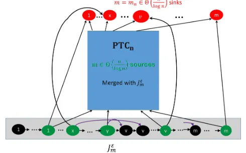
m). This process is illustrated in Figure 1b. We then obtain our final construction Gn, illustrated in Figure 1, by associating themsources ofPTCn with the nodes{2δv :v∈[m]} inJm, where >0 is fixed to be some suitably small constant.
It is straightforward to show thatJ
m is (e, δd)-depth robust for anye+d≤ (1−)m. Thus, it would be tempting that it will takeΩ(n) steps to (re)pebble c2n/lognsources during the interval [i, j] we obtain from Theorem 2. However, we still run into the same problem: In particular, suppose that at some point in timek we can find a setT ⊆ {2vδ:v∈[m]} \Pk with|T| ≥c2n/logn(e.g., a set of sources inPTCn) such that the longest path running throughT inJm −Pk has length less than c5n. If the interval [i, j] starts at time i =k+ 1 then we cannot ensure that it will take time≥c5nto (re)pebble thesec2n/lognsource nodes.
Claim 1 addresses this challenge directly. If such a problematic timekexists then Claim 1 implies that we must haveΠssk (P, Ω(n/logn)))∈Ω(n). At a high level the argument proceeds as follows: suppose that we find such a problem time k along with a set T ⊆ {2vδ : v ∈ [m]} \Pk with |T| ≥ c2n/logn such that depth(J
m[T]) ≤ c5n. Then for any time r ∈ [k−c5n, k] we know that the the length of the longest path running through T in J
m−Pr is at most
depth(J
m[T]−Pr)≤c5n+ (k−r) ≤2c5n since the depth can decrease by at most one each round. We can then use the extreme depth-robustness of D
m and the construction ofJ
(a) PTCn: a superconcentrator [PTC76] with m = Ω(n/logn) sources and
sinks and maximum space complexityΠsk(PTCn)∈Ω
n
logn
.
(b) Indegree Recution transforms -extreme depth robust graph D
m with
m nodes and indeg(Dm) ∈ O(logn) into indegree reduced graph Jm with
2indeg(D
m)×m∈O(n) nodes andindeg(Jm) = 2.
(c) Final ConstructionGn. OverlaymnodesJm withmsources inPTCn.
Fig. 1: BuildingGn withΠ k ss
Gn,logcnn
from Theorem 2 must have length at least i−j ≥c5n. In either case we have Πssk (P, Ω(n/logn)))≥Ω(n).
Proof of Theorem 1. We begin with the family of DAGs{PTCn}∞n=1 from The-orem 2. Fixing PTCn = ([n], En) we let S ={v ∈ [n] : parents(v) = ∅} ⊆ V denote the sources of this graph and we letc1, c2, c3 >0 be the constants from Theorem 2. Let ≤c2/(4c1). By Theorem 3 we can find a depth-robust DAG D
|S| on|S|nodes which is (a|S|, b|S|)-DR for anya+b ≤1− with indegree c0logn≤δ=indeg(D)≤c00log(n) for some constantsc0, c00. We letJ
|S| denote the indegree reduced version ofD
|S|from Lemma 1 with 2|S|δ∈O(n) nodes and
indeg= 2. To obtain our DAGGn fromJn and PTCn we associate each of the S nodes 2vδ inJ
n with one of the nodes inS. We observe thatGn has at most 2|S|δ+n∈O(n) nodes and thatindeg(G)≤max{indeg(PTCn),indeg(Jn)}= 2 since we do not increase the indegree of any node in J
n when overlaying and in Gn do not increase the indegree of any nodes other than the sourcesS from
PTCn (these overlayed nodes have indegree at most 2 inJn).
Let P = (P0, . . . , Pt) ∈ PGk be given and observe that by restricting Pi0 = Pi∩V(PTCn) ⊆ Pi we have a legal pebbling P0 = (P00, . . . , Pt0) ∈ P
k
PTCn for
PTCn. Thus, by Theorem 2 we can find an interval [i, j] during which at least c2n/lognnodes in S are (re)pebbled and∀k∈[i, j] we have|Pk| ≥c3n/logn. We use T =S∩Sj
x=iPx−Pi−1 to denote the source nodes ofPTCn that are (re)pebbled during the interval [i, j]. We now setc4=c2/4 andc5=c2c0/4 and consider two cases:
Case 1: We have depth(ancestorsGn−Pi(T)) ≥ |T|δ/4. In other words at
time i there is an unpebbled path of length ≥ |T|δ/4 to some node in T. In this case, it will take at least j −i ≥ |T|δ/4 steps to pebble T so we will have at least |T|δ/4 ∈ Ω(n) steps with at least c3n/logn pebbles. Because c5=c2c0/4 it follows that|T|δ/4≥c2c0n≥c5n. Finally, sincec4≤c2 we have Πss(P, c4n/logn)≥c5n.
Case 2: We have depth(ancestorsGn−Pi(T)) < |T|δ/4. In other words at
time i there is no unpebbled path of length ≥ |T|δ/4 to any node in T. Now Claim 1 directly implies thatΠss(P,|T| −|S| − |T|/2))≥δ|T|/4. This in turn implies that Πss(P,(c2/2)n/(logn)−|S|) ≥ δc2n/(2 logn). We observe that δc2n/(2 logn)≥c5nsince, we havec5=c2c0/4. We also observe that (c2/2)n/logn− |S| ≥ (c2/2−c1)n/logn≥(c2/2−c2/4)n/logn ≥c2n/(4 logn) =c4nsince |S| ≤ c1n/logn, ≤c2/(4c1) and c4 = c2/4. Thus, in this case we also have Πss(P, c4n/logn)≥c5n, which implies thatΠssk (Gn, c4n/logn)≥c5n. Claim 1 Let Dn be an DAG with nodesV (Dn) = [n], indegreeδ=indeg(Dn)
that is (e, d)-depth robust for all e, d > 0 such that e+d ≤ (1 −)n, let
Jn be the indegree reduced version of Dn from Lemma 1 with 2δ nodes and
indeg(J
n) = 2, let T ⊆ [n] and let P = (P1, . . . , Pt) ∈ P k J
n,∅
be a (pos-sibly incomplete) pebbling of J
n. Suppose that during some round i we have
depth ancestorsJ n−Pi
S
v∈T{2δv}
≤cδ|T|for some constant0< c < 12. Then
Proof of Claim 1. For each time steprwe letHr=ancestorsJ n−Pr
S
v∈T{2δv}
and letk < ibe the last pebbling step beforeiduring whichdepth(Gk)≥2c|T|δ. Observe that k−i ≥ depth(Hk)−depth(Hi) ≥cnδ since we can decrease the length of any unpebbled path by at most one in each pebbling round. We also observe thatdepth(Hk) =c|T|δsincedepth(Hk)−1≤depth(Hk+1)<2c|T|δ.
Letr∈[k, i] be given then, by definition ofk, we havedepth(Hr)≤2c|T|δ. Let Pr0 = {v ∈ V(D
n) : Pr∩[2δ(v −1) + 1,2δv] 6= ∅} be the set of nodes v∈[n] =V(D
n) such that the corresponding path 2δ(v−1) + 1, . . . ,2δv inJn contains at least one pebble at timer. By depth-robustness ofD
n we have
depth(Dn[T]−Pr0)≥ |T| − |Pr0| −n . (1) On the other hand, exploiting the properties of the indegree reduction from Lemma 1, we have
depth(Dn[T]−Pr0)δ≤depth(Hr)≤2c|T|δ . (2) Combining Equation 1 and Equation 2 we have
|T| − |Pr0| −n≤depth(Dn[T]−Pr0)≤2c|T|.
It immediately follows that|Pr| ≥ |Pr0| ≥ |T| −2c|T| −nfor eachr∈[k, i] and, therefore,Πssk (P,|T| −n−2c|T|)≥cδ|T|.
Remark 3. (On the Explicitness of Our Construction) Our construction of a fam-ily of DAGs with high sustained space complexity is explicit in the sense that there is a probabilistic polynomial time algorithm which, except with very small probability, outputs annnode DAGGthat has high sustained space complexity. In particular, Theorem 1 relies on an explicit construction of [PTC76], and the extreme depth-robust DAGs from Theorem 3. The construction of [PTC76] in turn uses an object called superconcentrators. Since we have explicit construc-tions of superconcentrators [GG81] the construction of [PTC76] can be made explicit. While the proof of the existence of a family of extremely depth-robust DAGs is not explicit the proof uses a probabilistic argument and can be adapted to obtain a probabilistic polynomial time which, except with very small prob-ability, outputs ann node DAGGthat is extremely depth-robust. In practice, however it is also desirable to ensure that there is a local algorithm which, on input v, computes the set parents(v) in time polylog(n). It is an open question whether any DAG G with high sustained space complexity allows for highly efficient computation of the set parents(v).
4
Better Depth-Robustness
In this section we improve on the original analysis of Erdos et al. [EGS75], who constructed a family of DAGs{Gn}∞
for us since we require that the subgraphGn[T] is also highly depth robust for any sufficiently large subset T ⊆Vn of nodes e.g., for any T such that |T| ≥ n/1000. For any fixed constant > 0 [MMV13] constructs a family of DAGs {G
n}∞n=1 which is (αn, βn)-depth robust for any positive constants α, β such thatα+β ≤1−but their construction has indegreeO log2n·polylog(logn)
. By contrast, our results in the previous section assumed the the existence of such a family of DAGs withindeg(G
n)∈O(logn).
In fact our family of DAGs is essentially the same as [EGS75] with one minor modification to make the construction for for alln >0. Our contribution in this section is an improved analysis which shows that the family of DAGs {G
n}∞n=1 with indegree O(logn) is (αn, βn)-depth robust for any positive constantsα, β such thatα+β ≤1−.
We remark that if we allow our family of DAGs to haveindeg(G
n)∈O(lognlog ∗n) then we can eliminate the dependence on entirely. In particular, we can con-struct a family of DAGs {Gn}∞
n=1 with indeg(Gn) = O(lognlog
∗n) such that for any positive constants such thatα+β <1 the DAGGn is (αn, βn)-depth robust for all suitably largen.
Theorem 3. Fix > 0 then there exists a family of DAGs {G
n}∞n=1 with
indeg(G
n) =O(logn)that is (αn, βn)-depth robust for any constantsα, β such
that α+β <1−.
The proof of Theorem 3 relies on Lemma 4, Lemma 5 and Lemma 6. We say thatGis aδ-local expander if for every nodex∈[n] and everyr≤x, n−xand every pair A⊆Ir(x)=. {x−r−1, . . . , x}, B⊆Ir∗(x)=. {x+ 1, . . . , x+r} with size|A|,|B| ≥δrwe haveA×B∩E 6=∅i.e., there is a directed edge from some node inAto some node inB. Lemma 4 says that for any constantδ >0 we can construct a family of DAGs{LEδn}∞
n=1withindeg=O(logn) such that eachLE δ n is aδ-local expander. Lemma 4 essentially restates [EGS75, Claim 1] except that we require thatLEnis aδ-local expander foralln >0 instead of fornsufficiently large. Since we require a (very) minor modification to achieveδ-local expansion for all n >0 we include the proof of Lemma 4 in the full version [ABP18] for completeness.
Lemma 4. [EGS75] Letδ >0be a fixed constant then there is a family of DAGs
{LEδn}∞n=1 withindeg∈O(logn)such that each LE δ
Lemma 5. Let G= (V = [n], E)be a δ-local expander and letx < y∈[n] both be γ-good under S ⊆[n] then ifδ <min{γ/2,1/4} then there is a directed path from node xto node y inG−S.
Lemma 6 shows thatalmost all of the remaining nodes in LEδn−S will be γ-good. It immediately follows thatLEn−S contains a directed path running throughalmost allof the nodes [n]\S. While Lemma 6 may appear similar to [EGS75, Claim 2] at first glance, we again stress one crucial difference. The proof of [EGS75, Claim 2] is only sufficient to show that at leastn−2|S|/(1−γ)≥ n−2|S| nodes areγ-good. At best this would allow us to conclude thatLEδn is (e, n−2e)-depth robust. Together Lemma 6 and Lemma 5 imply that ifLEδn is a δ-local expander (δ <min{γ/2,1/4}) thenLEδn is
e, n−e1+γ1−γ-depth robust. Lemma 6. For any DAGG= ([n], E)and any subsetS⊆[n]of nodes at least
n− |S|1+γ1−γ of the remaining nodes inGare γ-good with respect toS.
Proof of Theorem 3. By Lemma 4, for any δ > 0, there is a family of DAGs {LEδn}∞
n=1 withindeg
LEδn∈O(logn) such that for each n≥1 the DAGLEδn
is aδ-local expander. Given∈(0,1] we will setG n =LE
δ
nwithδ=/10<1/4 so that G
n is a (/10)-local expander. We also set γ =/4 >2δ. Let S ⊆Vn of size |S| ≤ebe given. Then by Lemma 6 at least n−e1+γ1−γ of the nodes are γ-good and by Lemma 5 there is a path connecting allγ-good nodes in G
n−S. Thus, the DAGG
n is
e, n−e1+γ1−γ-depth robust for anye≤n. In particular, ifα=e/n andβ = 1−α1+γ1−γ then the graph is (αn, βn)-depth robust. Finally we verify that
n−αn−βn=−e+eα1 +γ 1−γ =e
2γ 1−γ ≤n
2−/2 ≤n .
The proof of Lemma 5 follows by induction on the distance|y−x|between γ-good nodesxandy. Our proof extends a similar argument from [EGS75] with one important difference. [EGS75] argued inductively that for each good node xand for each r >0 over half of the nodes in Ir∗(x) are reachable from xand that xcan be reached from over half of the nodes inIr(x) — this implies that y is reachable from xsince there is at least one nodez ∈I|y−x|∗ (x) =I|y−x|(y) such that z can be reached from x and y can be reached from z in G−S. Unfortunately, this argument inherently requires that γ ≥0.5 since otherwise we may have at least |I∗
Claim 2 Let G = (V = [n], E) be a δ-local expander, let x ∈ [n] be a γ-good node under S ⊆[n] and let r > 0 be given. If δ < γ/2 then all but 2δr of the nodes in Ir∗(x)\S are reachable from x in G−S. Similarly, x can be reached from all but 2δr of the nodes in Ir(x)\S. In particular, if δ < 1/4 then more than half of the nodes inIr∗(x)\S (resp. in Ir(x)\S) are reachable fromx(resp.
xis reachable from) inG−S.
Proof. Claim 2 We prove by induction that (1) if r = 2kδ−1 for some integer k then all but δr of the nodes in Ir∗(x)\S are reachable from x and, (2) if 2k−1< r < 2kδ−1 then then all but 2δr of the nodes in I∗
r(x)\S are reachable from x. For the base cases we observe that if r≤δ−1 then, by definition of a δ-local expander, x is directly connected to all nodes in Ir∗(x) so all nodes in Ir(x)\S are reachable.
Now suppose that claims (1) and (2) holds for each r0 ≤r = 2kδ−1. Then we show that the claim holds for each r < r0 ≤ 2r = 2k+1δ−1. In particular, letA ⊆Ir∗(x)\S denote the set of nodes inIr∗(x)\S that are reachable fromx via a directed path inG−S and letB ⊆Ir∗0−r(x+r)\S be the set of all nodes in Ir∗0−r(x+r)\S that arenot reachablefromxin G−S. Clearly, there are no directed edges fromAtoBinGand by induction we have|A| ≥ |Ir∗(x)\S|−δr≥ r(γ−δ)> δr. Thus, byδ-local expansion|B| ≤rδ. Since,|Ir∗(x)\(S∪A)| ≤δr at most |Ir∗0(x)\(S∪A)| ≤ |B|+δr ≤ 2δr ≤ 2δr0 nodes in I2r∗ (x)\S are not reachable from xin G−S. Since,r0 > rthe number of unreachable nodes is at most 2δr≤2δr0, and ifr0= 2rthen the number of unreachable nodes is at most 2δr=δr0.
A similar argument shows thatxcan be reached from all but 2δrof the nodes
in Ir(x)\S in the graphG−S.
Proof of Lemma 5. By Claim 2 for each r we can reach |Ir∗(x)\S| −δr = |I∗
r(x)\S|
1−δ |Ir∗(x)|
|I∗
r(x)\S|
≥ |I∗ r(x)\S|
1−δ γ
> 1 2|I
∗
r(x)\S| of the nodes in Ir∗(x)\S from the node xin G−S. Similarly, we can reach y from more than
1
2|Ir(x)\S| of the nodes in Ir(y)\S. Thus, by the pigeonhole principle we can find at least one nodez∈I|y−x|∗ (x)\S=I|y−x|(y)\Ssuch thatzcan be reached
fromxandy can be reached fromz inG−S.
Lemma 6 shows that almost all of the nodes inG−S areγ-good. The proof is again similar in spirit to an argument of [EGS75]. In particular, [EGS75] constructed a superset T of the set of all γ-bad nodes and then bound the size of this superset T. However, they only prove that BAD ⊂ T ⊆ F ∪B where |F|,|B| ≤ |S|/(1−γ). Thus, we have |BAD| ≤ |T| ≤ 2|S|/(1−γ). Unfortunately, this bound is not sufficient for our purposes. In particular, if |S|=n/2 then this bound does not rule out the possibility that|BAD|=n so that none of the remaining nodes are good. Instead of bounding the size of the superset T directly we instead bound the size of the set T \S observing that |BAD| ≤ |T| ≤ |S|+|T\S|. In particular, we can show that|T\S| ≤ 2γ|S|1−γ. We then have|GOOD| ≥n− |T|=n− |S| − |T\S| ≥n− |S| −2γ|S|1−γ .
with a forward witness. Oncex∗1, r1∗, . . . , xk∗, r∗k have been define letx∗k+1 be the lexicographically least γ-bad node such that x∗k+1 > x∗k +rk∗ and x∗k+1 has a forward witness rk+1∗ (if such a node exists). Let x∗1, r∗1, . . . , x∗k, rk∗∗ denote the complete sequence, and similarly define a maximal sequencex1, r1, . . . , xk, rk of γ-bad nodes with backwards witnesses such thatxi−ri> xi+1 for eachi.
Let
F = k∗
[
i=1 Ir∗∗
i(x
∗
i) , and B= k
[
i=1 Iri(xi)
Note that for eachi≤k∗we have I
∗ r∗
i (x
∗ i)\S
≤γr. Similarly, for eachi≤kwe
have|Iri(xi)\S| ≤γr. Because the setsIr∗∗
i (x
∗
i) are all disjoint (by construction) we have
|F\S| ≤γ k∗
X
i=1
r∗i =γ|F|.
Similarly,|B\S| ≤γ|B|. We also note that at least (1−γ)|F|of the nodes in|F| are in |S|. Thus, |F|(1−γ) ≤ |S|and similarly |B|(1−γ)≤ |S|. We conclude that |F\S| ≤ γ|S|1−γ and that|B\S| ≤ γ|S|1−γ.
To finish the proof letT =F∪B=S∪(F\S)∪(B\S). Clearly,Tis a superset of all γ-bad nodes. Thus, at least n− |T| ≥ n− |S|1 + 1−γ2γ = n− |S|1+γ1−γ nodes are good.
We also remark that Lemma 4 can be modified to yield a family of DAGs {LEn}∞n=1 with indeg(LEn) ∈ O(lognlog∗n) such that each LEn is a δn local expander for some sequence {δn}∞n=1converging to 0. We can define a sequence {γn}∞n=1 such that
1+γn
1−γn converges to 1 and 2γn> δn for eachn. Lemma 4 and
Lemma 6 then imply that eachGnis
e, n−e1+γn
1−γn
-depth robust for anye≤n.
4.1 Additional Applications of Extremely Depth Robust Graphs
We now discuss additional applications of Theorem 3.
Application 1: Improved Proofs of Sequential Work As we previously noted Mahmoody et al. [MMV13] used extremely depth-robust graphs to con-struct efficient Proofs-Of-Sequential Work. In a proof of sequential work a prover wants to convince a verifier that he computed a hash chain of lengthninvolving the input value x without requiring the verifier to recompute the entire hash chain. Mahmoody et al. [MMV13] accomplish this by requiring the prover com-putes labelsL1, . . . , Ln by “pebbling” an extremely depth-robust DAGGn e.g., Li+1=H(xkLv1k. . .kLvδ) where{v1, . . . , vδ}=parents(i+ 1) andH is a
then either a (possibly cheating) prover make at least (1−)nsequential queries to the random oracle, or the the prover will fail to convince the verifier with high probability [MMV13].
We note that the parameter δ = indeg(Gn) is crucial to the efficiency of the Proofs-Of-Sequential Work protocol since each audit challenge requires the prover to revealδ+ 1 labels in the Merkle tree. The DAGGn from [MMV13] hasindeg(Gn)∈O log2n·polylog(logn)
while our DAGGn from Theorem 3 has maximum indegree indeg(Gn)∈O(logn). Thus, we can improve the com-munication complexity of their Proofs-Of-Sequential Work protocol by a factor ofΩ(logn·polyloglogn). However, Cohen and Pietrzak [CP18] found an alter-nate construction of a Proofs-Of-Sequential Work protocol that does not involve depth-robust graphs and which would almost certainly be more efficient than either of the above constructions in practice.
Application 2: Graphs with Maximum Cumulative Cost We now show that our family of extreme depth-robust DAGs has the highest possible cumu-lative pebbling cost even in terms of theconstantfactors. In particular, for any constantη >0 and < η2/100 the family{G
n}∞n=1of DAGs from Theorem 3 has Πcck (Gn)≥
n2(1−η)
2 andindeg(Gn)∈O(logn). By comparison,Π k
cc(Gn)≤n 2+n
2 foranyDAGG∈Gn — even ifGis the complete DAG.
Previously, Alwen et al. [ABP17] showed that any (e, d)-depth robust DAGG hasΠcck(G)> edwhich implies that there is a family of DAGGnwithΠcck(Gn)∈ Ω n2 [EGS75]. We stress that we need new techniques to prove Theorem 4. Even if a DAG G∈Gn were (e, n−e)-depth robust for every e≥0 (the only DAG actually satisfying this property is the compete DAG Kn) [ABP17] only implies thatΠcck(G)≥maxe≥0e(n−e) =n2/4. Our basic insight is that at time ti, the first time a pebble is placed on nodei in G
n, the node i+γiis γ-good and is therefore reachable via an undirected path from all of the other γ-good nodes in [i]. If we have|Pti|<(1−η/2)ithen we can show that at leastΩ(ηi) of the nodes in [i] areγ-good. We can also show that theseγ-good nodes form a depth robust subset and will cost Ω (η−)2i2
to repebble them by [ABP17]. Since, we would need to pay this cost by timeti+γiit is less expensive to simply ensure that|Pti|>(1−η/2)i. We refer an interested reader to Appendix A for a complete proof.
Theorem 4. Let 0 < η < 1 be a positive constant and let = η2/100 then the family {Gn}∞n=1 of DAGs from Theorem 3 has indeg(Gn) ∈ O(logn) and Πcck (Gηn)≥
n2(1−η) 2 .
when we can verify the correctness of this guess). Formally, black white-pebbling configuration Pi = PiW, PiB
of a DAG G = ([n], E) consists of two subsets PW
i , PiB ⊆[n] where PiB (resp. PiW) denotes the set of nodes in Gwith black (resp. white) pebbles on them at time i. For a legal parallel-black sequential-white pebbling P = (P0, . . . , Pt)∈ PBW
G we require that we start with no peb-bles on the graph i.e., P0 = (∅,∅) and that all white pebbles are removed by the end i.e.,PW
t =∅so that we verify the correctness of every nondeterministic guess before terminating. If we place a black pebble on a node v during round i+ 1 then we require that all ofv’s parents have a pebble (either black or white) on them during round i i.e., parents Pi+1B \PiB ⊆PiB∪PiW. In the Parallel-Black Sequential-White model we require that at most one new white pebble is placed on the DAG in every round i.e., PiW \Pi−1W
≤1 while no such restrict
applies for black pebbles.
We can use our construction of a family of extremely depth-robust DAG {G
n}∞n=1 to establish new upper and lower bounds for bounds for parallel-black sequential white pebblings.
Alwen et al. [AdRNV17] previously showed that in the parallel-black sequen-tial white pebbling model an (e, d)-depth-robust DAG G requires cumulative space at leastΠccBW(G)
.
= minP∈PBW G
Pt
i=1
PiB∪PiW ∈Ω
e√d or at least ≥edin the sequential black-white pebbling game. In this section we show that any (e, d)-reducible DAG admits a parallel-black sequential white pebbling with cumulative space at mostO(e2+dn) which implies that any DAG with constant indegree admits a parallel-black sequential white pebbling with cumulative space at most O(n2loglog22logn n) since any DAG is (nlog logn/logn, n/log
2n)-reducible. We also show that this bound is essentially tight (up to log lognfactors) using our construction of extremely depth-robust DAGs. In particular, by applying in-degree reduction to the family{Gn}∞n=1, we can find a family of DAGs{Jn}∞n=1 with indeg(J
n) = 2 such that any parallel-black sequential white pebbling has cumulative space at leastΩ(logn22n). To show this we start by showing that any parallel-black sequential white pebbling of an extremely depth-robust DAGG
n, withindeg(G)∈O(logn), has cumulative space at leastΩ(n2). We use Lemma 1 to reduce the indegree of the DAG and obtain a DAG J
n withn0 ∈O(nlogn) nodes andindeg(G) = 2, such that any parallel-black sequential white pebbling ofJn has cumulative space at leastΩ( n
2 log2n).
the next round e.g.,P1= (∅, V) andP2= (∅,∅). Thus, any DAG has cumulative space complexityθ(n) in the “parallel-white parallel-black” pebbling model.
Theorem 5 shows that (e, d)-reducible DAG admits a parallel-black sequen-tial white pebbling with cumulative space at most O(e2+dn). The basic peb-bling strategy is reminiscent of the parallel black-pebpeb-bling attacks of Alwen and Blocki [AB16]. Given an appropriate depth-reducing setSwe use the firste=|S| steps to place white pebbles on all nodes inS. SinceG−S has depth at most d we can place black pebbles on the remaining nodes during the next dsteps. Finally, once we place pebbles on every node we can legally remove the white pebbles. A formal proof of Theorem 5 can be found in Appendix A.
Theorem 5. Let G= (V, E) be (e, d)-reducible thenΠccBW(G)≤ e(e+1)
2 +dn.
In particular, for any DAG G with indeg(G) ∈ O(1) we have ΠccBW(G) ∈ O
nlog logn
logn
2
.
Theorem 6 shows that our upper bound is essentially tight. In a nut-shell their lower bound was based on the observation that for any integers i, d the DAG G−S
jPi+jd has depth at most d since any remaining path must have been pebbled completely in timed— ifGis (e, d)-depth robust this implies that
S
jPi+jd
≥e. The key difficulty in adapting this argument to the parallel-black
sequential white pebbling model is that it is actually possible to pebble a path of lengthdinO(√d) steps by placing white pebbles on every interval of length√d. This is precisely why Alwen et al. [AdRNV17] were only able to establish the lower boundΩ(e√d) for the cumulative space complexity of (e, d)-depth robust DAGs — observe that we always havee√d≤n1.5sincee+d≤nfor any DAG G. We overcome this key challenge by using extremely depth-robust DAGs.
In particular, we exploit the fact that extremely depth-robust DAGs are “recursively” depth-robust. For example, if a DAGG is (e, d)-depth robust for anye+d≤(1−)nthen the DAGG−Sis (e, d)-depth robust for anye+d≤(n− |S|)−n. SinceG−S is still sufficiently depth-robust we can then show that for some nodex∈V(G−S) any (possibly incomplete) pebblingP = (P0, P1, . . . , Pt) of G−S with P0 = Pt = (∅,∅) either (1) requires t ∈ Ω(n) steps, or (2) fails to place a pebble on x i.e. x /∈ St
r=0 P W 0 ∪PrB
. By Theorem 3 it then follows that there is a family of DAGs{Gn}∞n=1withindeg(Gn)∈O(logn) and ΠccBW(G)∈Ω(n2). If apply indegree reduction Lemma 1 to the family{Gn}∞n=1 we obtain the family {J
n}∞n=1 with indeg(Jn) = 2 and O(n) nodes. A similar argument shows that ΠBW
cc (Jn)∈Ω(n2/log
2n). A formal proof of Theorem 6 can be found in Appendix A.
Theorem 6. Let G = (V = [n], E ⊃ {(i, i+ 1) : i < n}) be (e, d) -depth-robust for any e+d≤(1−)n thenΠccBW(G)≥(1/16−/2)n2. Furthermore,
if G0 = ([2nδ], E0) is the indegree reduced version of G from Lemma 1 then ΠBW
cc (G0)≥(1/16−/2)n2. In particular, there is a family of DAGs{Gn}∞n=1
with indeg(Gn) ∈ O(logn) and ΠccBW(G) ∈ Ω(n2), and a separate family of
DAGs {Hn}∞
n=1 withindeg(Hn) = 2 andΠ BW
cc (Hn)∈Ω
n2 log2n
5
A Pebbling Reduction for Sustained Space Complexity
As an application of the pebbling results on sustained space in this section we construct a new type of moderately hard function (MoHF) in the parallel ran-dom oracle model pROM. In slightly more detail, we first fix the computational model and define a particular notion of moderately hard function called sustained memory-hard functions (SMHF). We do this using the framework of [AT17] so, beyond the applications to password based cryptography, the results in [AT17] for building provably secure cryptographic applications on top of any MoHF can be immediately applied to SMHFs. In particular this results in a proof-of-work and non-interactive proof-of-proof-of-work where “proof-of-work” intuitively means having performed some computation entailing sufficient sustained memory. Finally we prove a “pebbling reduction” for SMHFs; that is we show how to bound the parameters describing the sustained memory complexity of a family of SMHFs in terms of the sustained space of their underlying graphs.8
We note that the pebbling reduction below caries over almost unchanged to the framework of [AS15]. That is by defining sustained space in the compu-tational model of [AS15] similarly to the definition below a very similar proof to that of Theorem 7 results the analogous theorem but for the [AT17] frame-work. Never-the-less we believe the [AT17] framework to result in a more useful definition as exemplified by the applications inherited from that work.
5.1 Defining Sustained Memory Hard Functions
We very briefly sketch the most important parts of the MoHF framework of [AT17] which is, in turn, a generalization of the indifferentiability framework of [MRH04].
We begin with the following definition which describes a family of functions that depend on a (random) oracle.
Definition 6 (Oracle functions).For (implicit) oracle setH, an oracle
func-tion f(·) (with domain D and range R), denoted f(·) : D → R, is a set of functions indexed by oracles h∈Hwhere each fh mapsD→R.
Put simply, an MoHF is a pair consisting of an oracle family f(·) and an honest algorithm N for evaluating functions in the family using access to a random oracle. Such a pair is secure relative to some computational modelM if no adversary Awith a computational device adhering to M (denoted A ∈M) can produce output which couldn’t be produced simply by calledf(h)a limited number of times (wherehis a uniform choice of oracle fromH). It is asumed that algorithmN is computable by devices in some (possibly different) computational model ¯M when given sufficent computational resources. Usually M is strictly more powerful than ¯M reflecting the assumption that an adversary could have a more powerful class of device than the honest party. For example, in this work we will let model ¯M contain only sequential devices (say Turing machines which
8
make one call to the random oracle at a time) whileM will also include parallel devices.
In this work, both the computational modelsM and ¯M are parametrized by the same space P. For each model, the choice of parameters fixes upperbounds
on the power of devices captured by that model; that is on the computational resources available to the permitted devices. For exampleMacould be all Turing machines making at mostaqueries to the random oracle. The security of a given moderatly hard function is parameterized by two functionsαandβ mapping the parameter space for M to positive integers. Intuitively these functions are used to provide the following two properties.
Completeness: To ensure the construction is even useable we require thatN is (computable by a device) in modelMa and thatN can evaluatef(h)(when given access toh) on at leastα(a) distinct inputs.
Security: To capture how bounds on the resources of an adversary A limit
the ability ofAto evalute the MoHF we require that the output ofAwhen running on a device in modelMb (and having access to the random oracle) can be reproduced by some simulator σ using at most β(b) oracle calls to f(h) (for uniform randomly sampledh←H.
To help build provably secure applications on top of MoHFs the framework makes use of a destinguisher D (similar to the environment in the Universal Composability[Can01] family of models or, more accurately, to the destinguisher in the indifferentiability framework). The job ofDis to (try to) tell areal world
interaction with N and the adversaryA apart from an ideal world interaction withf(h)(in place ofN) and a simulator (in place of the adversary). Intuitivelly, D’s access to N captures whatever D could hope to learn by interacting with an arbitrary application making use of the MoHF. The definition then ensures that even leveraging such information the adversaryAcan not produce anything that could not be simulated (by simulator σ) to Dusing nothing more than a few calls tof(h).
As in the above description we have ommited several details of the framework we will also use a somewhat simplified notation. We denote the above described real world execution with the pair (N,A) and an ideal world execution where D is permited c ∈ N calls to f(·) and simulator σ is permited d ∈ N calls to f(h) with the pair (f(·), σ)
c,d. To denote the statement that no D can tell an interaction with (N,A) apart one with (f(·), σ)c,dwith more than probability we write (N,A)≈(f(·), σ)c,d.
Finally, to accomadate honest parties with varying amounts of resources we equip the MoHF with a hardness parametern∈N. The following is the formal
Definition 7 (MoHF security). LetM andM¯ be computational models with bounded resources parametrized by P. For each n ∈ N, let fn(·) be an oracle
function and N(n,·) be an algorithm (computable by some device in M¯) for evaluating fn(·). Let α, β : P×N → N, and let : P×P×N → R≥0. Then, (fn(·),Nn)n∈N is a (α, β, )-secure moderately hard function family (for model
M)if
∀n∈N,r∈P,A ∈Mr ∃σ∀l∈P: (N(n,·),A) ≈(l,r,n) (fn(·), σ)α(l,n),β(r,n), (3)
The function family is asymptotically secure if (l,r,·) is a negligible function in the third parameter for all values of r,l∈P.
Sustained Space Constrained Computation. Next we define the honest and ad-versarial computational models for which we prove the pebbling reduction. In particular we first recall (a simplified version of) the pROM of [AT17]. Next we define a notion of sustained memory in that model naturally mirroring the notion of sustained space for pebbling. Thus we can parametrize the pROM by memory thresholdsand timetto capture all devices in the pROM with no more sustained memory complexity then given by the choice of those parameters.
In more detail, we consider a resource-bounded computational deviceS. Let w ∈ N. Upon startup, Sw-prom samples a fresh random oracle h←$Hw with range{0,1}w. Now Sw-prom accepts as input a pROM algorithm Awhich is an oracle algorithm with the following behavior.
A stateis a pair (τ,s) where data τ is a string and s is a tuple of strings. The output of step iof algorithm Ais anoutput state σi¯ = (τi,qi) where qi= [qi1, . . . , qzi
i ] is a tuple ofqueriestoh. As input to stepi+ 1, algorithmAis given the corresponding input stateσi = (τi, h(qi)), whereh(qi) = [h(q1i), . . . , h(q
zi
i )] is the tuple ofresponsesfromhto the queriesqi. In particular, for a givenhand random coins ofA, the input stateσi+1 is a function of the input stateσi. The initial stateσ0 is empty and the inputxin to the computation is given a special
input in step 1.
For a given execution of a pROM, we are interested in the following new complexity measure parametrized by an integer s ≥ 0. We call an element of {0,1}s a block. Moreover, we denote the bit-length of a string r by |r|. The
lengthof a stateσ= (τ,s) withs= (s1, s2, . . . , sy) is|σ|=|τ|+P
i∈[y]|s
i|. For a given stateσletb(σ) =b|σ|/scbe the number of “blocks inσ”. Intuitively, thes -sustained memory complexity (s-SMC) of an execution is the sum of the number of blocks in each state. More precisely, consider an execution of algorithmAon inputxinusing coins $ with oraclehresulting inz∈Z≥0input statesσ1, . . . , σz, where σi = (τi,si) and si = (s1i, s2i, . . . , s
yj
i ). Then the for integer s ≥ 0 the s-sustained memory complexity (s-SMC) of the execution is
s-smc(Ah(x
in; $)) =
X
while thetotal number of RO calls isP
i∈[z]yj. More generally, thes-SMC (and total number of RO calls) of several executions is the sum of the s-sMC (and total RO calls) of the individual executions.
We can now describe the resource constraints imposed by Sw-prom on the pROM algorithms it executes. To quantify the constraints,Sw-promis parametrized by element fromPprom=N3which describe the limites on an execution of
algo-rithmA. In particular, for parameters (q, s, t)∈Pprom, algorithm Ais allowed
to make a total of q RO calls and have s-SMC at most t (summed across all invocations ofAin any given experiment).
As usual for moderately hard functions, to ensure that the honest algorithm can be run on realistic devices, we restrict the honest algorithmN for evaluating the SMHF to be asequential algorithms. That is,N can make only a single call tohper step. Technically, in any execution, for any stepjit must be thatyj≤1. No such restriction is placed on the adversarial algorithm reflecting the power (potentially) available to such a highly parallel device as an ASIC. In symbols we denote the sequential version of the pROM, which we refer to as the sequential ROM (sROM) bySw-srom.
We can now (somewhat) formally define of a sustained memory-hard function for the pROM. The definition is a particular instance of and moderately hard function (c.f. Definition 7).
Definition 8 (Sustained Memory-Hard Function). For each n ∈ N, let
fn(·) be an oracle function and Nn be an sROM algorithm for computing f(·).
Consider the function families:
α={αw:Pprom×N→N}w∈N, β={βw:Pprom×N→N}w∈N,
={w:Pprom×Pprom×N→N}w∈N.
Then F = (fn(·),Nn)n∈N is called an (α, β, )-sustained memory-hard function (SMHF) if ∀w∈NF is an(αw, βw, w)-secure moderately hard function family forSw-prom.
5.2 The Construction
In this work f(·) will be a graph function [AS15] (also sometimes called “hash graph”). The following definition is taken from [AT17]. A graph function depends on an oracle h ∈ Hw mapping bit strings to bit strings. We also assume the existance of an implicit prefix-free encoding such thathis evaluated on unique strings. Inputs tohare given as distinct tuples of strings (or even tuples of tuples of strings). For example, we assume that h(0,00), h(00,0), and h((0,0),0) all denote distinct inputs toh.
Definition 9 (Graph function).Let functionh:{0,1}∗→ {0,1}w∈
Hwand
DAGG= (V, E)have source nodes{vin