An Algorithmic Framework for the Generalized
Birthday Problem
Itai Dinur
Department of Computer Science, Ben-Gurion University, Israel
Abstract. The generalized birthday problem (GBP) was introduced by Wagner in 2002 and has shown to have many applications in cryptanaly-sis. In its typical variant, we are given access to a functionH :{0,1}`→
{0,1}n
(whose specification depends on the underlying problem) and an integerK >0. The goal is to findK distinct inputs toH (denoted by {xi}K
i=1) such that
PK
i=1H(xi) = 0. Wagner’s K-tree algorithm solves the problem in time and memory complexities of aboutN1/(blogKc+1)
(whereN = 2n). Two important open problems raised by Wagner were (1) devise efficient time-memory tradeoffs for GBP, and (2) reduce the complexity of the K-tree algorithm forKwhich is not a power of 2. In this paper, we make progress in both directions. First, we improve the best know GBP time-memory tradeoff curve (published by indepen-dently by Nikoli´c and Sasaki and also by Biryukov and Khovratovich) for allK≥8 fromT2MblogKc−1
=N toTd(logK)/2e+1
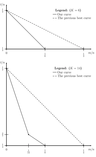
Mb(logK)/2c =N, applicable for a large range of parameters. For example, forK= 8 we improve the best previous tradeoff fromT2M2 =N to T3M =N and forK= 32 the improvement is fromT2M4=N toT4M2=N. Next, we consider values ofKwhich are not powers of 2 and show that in many cases even more efficient time-memory tradeoff curves can be obtained. Most interestingly, forK∈ {6,7,14,15}we present algorithms with the same time complexities as the K-tree algorithm, but with signif-icantly reduced memory complexities. In particular, forK= 6 the K-tree algorithm achievesT = M =N1/3, whereas we obtain T = N1/3 and
M =N1/6. ForK = 14, Wagner’s algorithm achievesT =M =N1/4, while we obtainT =N1/4 andM =N1/8. This gives the first significant improvement over the K-tree algorithm for smallK.
Finally, we optimize our techniques for several concrete GBP instances and show how to solve some of them with improved time and memory complexities compared to the state-of-the-art.
Our results are obtained using a framework that combines several algo-rithmic techniques such as variants of the Schroeppel-Shamir algorithm for solving knapsack problems (devised in works by Howgrave-Graham and Joux and by Becker, Coron and Joux) and dissection algorithms (published by Dinur, Dunkelman, Keller and Shamir). It then builds on these techniques to develop new GBP algorithms.
1
Introduction
The generalized birthday problem (GBP) is a generalization of the classical birth-day problem of finding a collision between two elements in two lists, introduced by Wagner in 2002 [19]. Since its introduction, Wagner’s K-tree algorithm for GBP has become a widely applicable tool used in cryptanalysis of code-based cryptosystems [3] (that are important designs in post-quantum cryptography), hash functions (such as FSB [5]) and stream ciphers, where it is used as a proce-dure in fast correlation attacks [9, 14]. Furthermore, it is an important component in improved algorithms for hard instances of the knapsack problem [2, 13]. The K-tree algorithm is also closely related to the BKW algorithm for the learning parity with noise (LPN) problem [7], and the BKW extension to the learning with errors (LWE) problem [1].
We consider the most relevant GBP variant in cryptanalysis. For integer parameters K > 0 and 0 ≤ ` ≤ n, we are given access to a function H :
{0,1}`→ {0,1}n, and the goal is to findK distinct inputs toH,{xi}K i=1, such that PK
i=1H(xi) = 0. For simplicity, we assume that addition is performed bitwise overGF(2), but our algorithms easily extend to work with addition over
GF(2n). We further assume thatKnand treat it as a constant. We viewH
as a random oracle whose outputs are selected independently and uniformly at random from{0,1}n. The number ofK-tuples over`-bit words is about 2K`, and
as the problem places ann-bit constraint on the solution, the expected number of solutions is 2K`−n. In particular, we expect a solution only ifK`≥n. ForK≥2,
the problem can be solved in time 2n/2 using a simple collision search. Wagner’s observation was that for values ofK≥4, the problem can be solved much more efficiently assuming that the number of expected solutions is sufficiently large.
Wagner’s K-tree algorithm forK= 2k(wherekis a positive integer) receives
as inputK lists{Li}K
i=1, each containing about 2n/(k+1)strings ofnbits, which are assumed to be uniform in{0,1}n. The algorithm returns aK-tuple{yi}K
i=1, where yi∈Li such that PK
i=1yi = 0. The algorithm can be used to solve GBP assuming that ` ≥ n/(k+ 1) by initializing the lists {Li}K
i=1 with elements of the formy=H(x) for arbitrary values ofx∈ {0,1}`.
At a high level, the K-tree algorithm merges its 2k inputs lists in a full
binary tree structure withk layers. In each layer, the lists are merged in pairs, where each merged pair gives a new list that is input to the next layer and contains words with a larger zero prefix. Finally, the last layer yields a zero word which can be traced back to aK-tuple{xi}K
i=1such that
PK
i=1H(xi) = 0 as required. The time and memory complexities of the K-tree algorithm are about 2n/(k+1)=N1/(logK+1)(up to constants and small multiplicative factors in n, K), as detailed in Section 3. Since any GBP algorithm for a certain value of K can be extended with the same complexity to any K0 > K, the time and memory complexities of the K-tree algorithm for general K are N1/(logK+1), where logK is rounded down to the nearest integer.
2n/(k+1) memory. The trivial time-memory tradeoff algorithm repeatedly builds
K lists of sizeM from arbitrary inputs toH and executes the K-tree algorithm until a solution is found. Simple analysis shows that this algorithm achieves a tradeoff of T MlogK =N, which is very inefficient even whenK is moderately
large, as the time complexityT increases sharply for memoryM < N1/(logK+1). Improved tradeoffs were first published in [4, 5] (by Bernstein and Bernstein et al., respectively), where the main idea is to execute (what we call) a prepa-ration phase before running the K-tree algorithm. This phase iterates over a portion of the domain space and builds lists that are input to the K-tree algo-rithm (rather than building them arbitrarily), thus increasing its probability to find a solution. A different approach to the preparation phase based on partial collisions in H was published independently by Nikoli´c and Sasaki [16] and by Biryukov and Khovratovich [6]. This technique gives the currently best known GBP time-memory tradeoff ofT2MlogK−1=N.
Another challenge for GBP is the improve the K-tree algorithm for values of
Kthat are not powers of 2. While it is known how to achieve small (polynomial in n) savings in the GBP time complexity for some values ofK (e.g., see [16]), obtaining exponential improvements innremains an open problem.
In an additional practical setting, the domain size L = 2` of H is limited
and the K-tree algorithm cannot be directly applied. The best known algorithm for such cases is an extension of the K-tree algorithm, published by Minder and Sinclair [15]. In this context, we also mention the recent work of Both and May [8] which analyzed GBP instances generated by the parity check problem, which is an important problem in stream cipher cryptanalysis that can be reduced to GBP. Both and May developed a specific optimization technique for the parity check problem and used it to improve upon the extended K-tree algorithm for several GBP instances with values ofK that are not powers to 2.
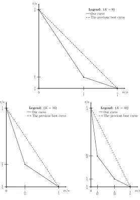
In this paper, we improve the state-of-the-art with respect to the aforemen-tioned challenges. Some of our results are summarized at a high level below, while our full tradeoff curves forK∈ {8,16,32,6,14}are plotted in Appendix F.
1. We devise a sub-linear1 time-memory tradeoff Td(logK)/2e+1Mb(logK)/2c =
N for GBP with K ≥ 8. This improves upon the currently best known tradeoffT2MlogK−1=N for allK≥8. Our tradeoff is applicable whenever
T1/2≤M ≤T. For the range 1< M ≤T1/2, we also improve upon the best known tradeoff forK≥8, but our curve formula becomes more complex as
K grows. We further improve these tradeoffs for values of K that are not powers of 2. Some examples are described below.
2. We devise the tradeoffT2M2=N forK= 6 (andK = 7), which improves upon the currently best tradeoff of T2M = N (obtained by the formula
T2MlogK−1=N usingK= 4) for the full range 1< M ≤T1/2.
3. In particular, for K = 6 (and K = 7) we achieve T =N1/3, M =N1/6, reducing to a square root the memory complexity of the best GBP algorithm, which obtainsT =M =N1/3 using the K-tree algorithm forK= 4. 1
4. We devise the tradeoffT3M2=N forK= 14 (andK= 15), which improves upon the currently best tradeoff of T2M2 = N (obtained by the formula
T2MlogK−1 = N using K = 8) for the range T1/4 ≤M ≤T1/2. We also obtain the improved tradeoffT2M6=N for the range 1≤M ≤T1/4. 5. In particular, for K = 14 (andK = 15) we achieve T =N1/4,M =N1/8,
reducing to a square root the memory complexity of the best GBP algorithm which obtainsT =M =N1/4 using the K-tree algorithm forK= 8. 6. We consider concrete GBP instances with a limited domain sizeL, recently
analyzed by Both and May [8] and show how to solve some (but not all) of them more efficiently, improving both the time and memory complexi-ties. Unlike Both and May’s technique (which is specific to the parity check problem) our algorithms can be applied to any GBP instance, achieving im-provements over the extended K-tree algorithm [15] for many values ofK
that are not powers to 2.
As noted above, previous time-memory tradeoffs applied apreparation phase to initialize several lists and search for a solution among them in (what we call) a list sum phase. In these works the focus was placed on the preparation phase, while the list sum phase applied the K-tree algorithm. In contrast, we focus on the list sum phase and develop algorithms that are superior to the straightforward application of the K-tree algorithm when the available memory is limited. We then carefully combine these algorithms with previous preparation phase techniques to obtain improved time-memory tradeoffs for GBP.
We begin by considering alist sum problem whose input consists ofKsorted lists{Li}Ki=1ofn-bit words and the goal is to find a certain number ofK-tuples {yi}Ki=1, whereyi∈Li such thatP
K
i=1yi = 0. There are severalexhaustive list
sum memory-efficient algorithms known for this problem that output all solu-tions. These algorithms are the starting points of the framework we develop in this paper. Our framework transforms such an exhaustive list sum algorithm into an efficient GBP algorithm for a given amount of memory. Obviously, an exhaus-tive list sum algorithm can be directly applied to solve GBP (after initializing
{Li}K
i=1accordingly), as the goal is to find only one out of all solutions. However, this trivial application is inefficient since it does not exploit the fact that we only search for a single solution and moreover, it does not use a preparation phase.
Our framework consists of three main parts. First, we transform a given exhaustive list sum algorithm to efficiently output a limited number of solutions, obtaining abasic list sum algorithm, optimized for a specific value ofK=P.
There are two classes of exhaustive memory-efficient list sum algorithms rel-evant to this work: the first class consists of variants of the Schroeppel-Shamir algorithm for solving knapsacks, devised by Howgrave-Graham and Joux [13] (which focused on K = 4) and by Becker, Coron and Joux [2] (which applied a recursive variant for K = 16). The second class consists of dissection algo-rithms [10], published by Dinur et al. and used to efficiently solve certain search problems with limited amount of memory.
solutions to solve the original problem. The difference between the classes is in the way the problem is partitioned: while Schroeppel-Shamir variants partition problem symmetrically into subproblems of equal sizes, dissection algorithms partition the problem asymmetrically into smaller and larger subproblems. Thus, Schroeppel-Shamir variants work best on values of K which are powers of 2, while dissection works best on “magic numbers” ofK(which are not necessarily powers of 2) such as 7 and 11 that exhibit ideal asymmetric partitions.
While the first part of the framework builds basic list sum algorithms for specific values ofK=P, the second part composes basic algorithms in alayered tree structure. This gives optimized list sum algorithms for values of K =Pk
(and additional values) where k is a positive integer. Finally, after optimizing the list sum phase, we combine it with a preparation phase to obtain a memory-efficient GBP algorithm. Methodologically, we make the following contributions: 1. We generalize and tie together several existing algorithmic techniques in a consistent framework: Section 2 introduces new algorithmic classification and notation and Section 3 presents prior work in a very structured way based on this classification. While these are preliminary sections, they already contain a non-trivial contribution that allows to construct new list sum algorithms in the subsequent parts of this paper in a relatively simple manner.
2. We transform the (symmetric) exhaustive Schroeppel-Shamir variants of [2, 13] to basic list sum algorithms for all values ofKthat are powers of 2. This generalizes the transformation forK= 4 by Howgrave-Graham and Joux. 3. We devise new algorithms that extend the dissection framework to GBP.
We further highlight the subtle differences in the ways that symmetric and asymmetric exhaustive list sum algorithms are transformed to solve GBP. Prior to this work dissection algorithms could not be efficiently applied to GBP as their complexity was at least 2n/2, which is a substantial limitation. 4. Analytically, we derive formulas that allow comparing competing list sum
(and consequently GBP) algorithms for various parameter values.
Even though the focus of this work is on memory-efficient GBP algorithms, for many concrete instances our techniques yield improvements in both time and memory complexities compared to the extended K-tree algorithm [15] (which is the current state-of-the-art). This occurs for values ofKwhich are not powers of 2 (such asK= 7), where our new algorithms extend the dissection framework. Such an improvement is surprising as standard dissection algorithms are time-memory tradeoffs which cannot improve the best time complexity of solving a problem given unlimited memory. The time complexity improvement is due to the fact that symmetric algorithms round the value of K down to the nearest power of 2 and ignore many of the possible solutions. On the other hand, the efficiency of GBP algorithms depends on their ability to find one out of many solutions, and ignoring a large fraction of them in advance is a suboptimal ap-proach. This further highlights the contribution of our third item above.
can be substantially reduced, whereas memory complexity remains unchanged. This gives yet another advantage to our time-memory tradeoff curves (partic-ularly to points such as T =M2) over the classical memory-consuming K-tree algorithm. Second, our framework can be extended to solve the LPN and LWE problems that are closely related to GBP. Preliminary analysis suggests that it improves several LPN time-memory tradeoffs recently obtained in [11]. Moreover, this work opens the door for efficient application of asymmetric (dissection-like) algorithms to LPN, whereas their complexity was previously too high to be competitive.
The rest of the paper is organized as follow. In Section 2 we introduce our notations and conventions, and describe preliminaries and previous work in Sec-tion 3. The first part of our framework that transforms exhaustive list sum algorithms to basic ones is introduced in Section 4, while the second part that constructs new layered algorithms is described in Section 5. In Section 6 we focus on the third part of the framework that combines preparation and list sum phase algorithms to solve GBP. Finally, in Section 7 we apply our new algorithms to concrete GBP instances and conclude the paper in Section 8.
2
Notations and Conventions
Given ann-bit stringx, we label its bits asx[1], x[2], . . . , x[n] (wherex[1] is the least significant bit or LSB). Given integers 1≤a≤b≤n, we denote byx[a–b] the (b−a+ 1)-bit stringx[a], x[a+ 1], . . . , x[b].
Let F : {0,1}` → {0,1}n, be a function for ` ≤ n . Given parameters `0 ≤` and n0 ≤n, define the truncated function F|`0,n0 : {0,1}`
0
→ {0,1}n0
as
F|`0,n0(x0) = F(x)[1–n0] (where the `-bit string xis constructed by appending `−`0 zero most significant bits to the`0-bit stringx0).
The generalized birthday problem (GBP). GBP with parameterKis given oracle access a function H :{0,1}` → {0,1}n for `≤n, and the goal is to find aK
-tuple {xi}Ki=1, wherexi ∈ {0,1}` are distinct (i.e.,xi6=xj fori6=j) such that
PK
i=1H(xi) = 0. The addition is performed bitwise overGF(2).
We assume in this paper thatH is a pseudo-random function. Our goal is to optimize the time complexityT of solving GBP with parametersKand`, given
M = 2mwords of memory, each of lengthnbit. In some settings (such as in [5])
eachxi in the outputK-tuple needs to come from a different domain. This can be modeled using K functions {Hi}K
i=1. The adaptation of the algorithms we consider to this setting is mostly straightforward.
Typically, GBP algorithms evaluate the functionH in a preparation phase in order to set up an instance of the list sum problem.
The list sum problem. Given K sorted lists {Li}Ki=1, each of M = 2m words (chosen uniformly at random) of length at least n, the goal is to find S (one, several, or all) K-tuples {yi}K
i=1, where yi ∈Li such that (
PK
in our framework list sum algorithms use aboutM = 2m memory (which is the
input size, up to the constantK).2
The list sum problem is related to the well-known K-SUM problem, which searches for a single solutionPK
i=1yi= 0 in one input set, as opposed to several lists. Moreover, typically the distribution of words in the input set of theK-SUM problem is arbitrary and it is a worst case problem (whereas we are interested in average case complexity).
Naming Conventions and Notations for List Sum Algorithms An algo-rithm that finds all solutions to the list sum problem is called anexhaustivelist sum algorithm. Otherwise, we name algorithms that output a limited number of solutions (with a bound on S) according to their internal structure: in general we havebasic algorithms andlayered algorithms that compose basic algorithms in a tree structure (similarly to the K-tree algorithm).
We refer to a list sum algorithm that solves the list sum problem for a specific value ofKas aK-way list sum algorithm. However, when referring to specific list sum algorithms we mostly need more refined notation that distinguishes them according to the values ofKandS (the number of required solutions) and also the type of basic algorithms composed in layered algorithms (which determine the arity of the tree). These parameters are sufficient to uniquely identify each list sum algorithm considered in this paper.
The (unique) non-layered list sum algorithm with parametersK, Sis denoted byAK,S, whereS is the number of solutions it produces. In case the algorithm is exhaustive (outputs all solutions), we simply writeAK. For example,A4 is an exhaustive 4-way list sum algorithm, whileA4,1produces only a single solution (and hence can be naturally used to solve GBP withK= 4).3In general, we will be interested in exhaustiveAK algorithms, basic AK,1 algorithms that output a single solution and basic AK,2m algorithms that produce S = 2m solutions,
allowing to compose basic algorithms and form layered ones.
The (unique) layered list sum algorithm withS= 1 and arity P is denoted by APK (we do not consider layered algorithms with S > 1 in this paper). For example, the K-tree algorithm is denoted by A2K, as it merges its input lists in pairs. We note that layered algorithms can be uniquely distinguished by their arity P, while K is left is symbolic form (unlike basic algorithms). We also remark that for any specific value ofK, the algorithmAK
K has a single layer and
is actually the basic algorithmAK,1 (which is our preferred notation).
When composing basic list sum algorithms in layers, the LSBs of the words in the input lists to the algorithms may already be zeroed by a previously applied 2 This definition does not capture algorithms (such as Minder and Sinclair’s algo-rithm [15]) that merge the initial lists into larger ones. However, the restriction typically does not result in loss of generality, as an initial merge can be considered as a preparation phase algorithm by defining the functionH appropriately. 3 When the number of expected solutions to the list sum problem isS, thenAK,S
basic algorithm and the task of the succeeding basic algorithm is to output solutions where the next sequence of bits is nullified. In such cases, we can ignore the zero LSBs in the input lists, resulting in a problem that complies with the above definition of list merge problem (which requires nullifying LSBs).
Complexity Evaluation The time and memory complexities of our algorithms are functions of the parameters n and K (and also L = 2` for some GBP
in-stances). We assume that Knand treat it as a constant. In the complexity analysis, we ignore multiplicative polynomial (and constant) factors innandK, which is common practice in exponential-time algorithms. Nevertheless, we note that these factors are relatively small for the algorithms considered.
On the other hand, when evaluating the complexity of our algorithms on concrete GBP instances in Section 7, we multiply both of their time and memory complexities byK in order to allow fair comparison to previous work.
3
Preliminaries and Previous Work
The literature relevant to this work is vast. In this section we summarize it con-structively so we can build upon it in the rest of this paper. We first describe general properties of list sum algorithms in Subsection 3.1. Then, we describe previous exhaustive list sum algorithmsAK: in Subsection 3.2 we focus on ex-haustive symmetric Schroeppel-Shamir variants for several values ofKwhich are powers of 2 (K∈ {4,16}and the basic K= 2), while in Subsection 3.3 we deal with asymmetric exhaustive dissection algorithms. In Subsection 3.4, we show how exhaustive algorithms for K = 2 and K = 4 were efficiently adapted to basic algorithms that output a limited number of solutions. In Subsection 3.5, we describe the (layered) K-tree algorithm. Next, in Subsection 3.6 we focus on the preparation phase algorithms parallel collision search (PCS) and clamp-ing through precomputation (CTP). We end this section by summarizclamp-ing the currently best known time-memory tradeoff for GBP in Subsection 3.7.
3.1 General Properties of List Sum Algorithms
From a combinatorial viewpoint, the number ofK-tuples{yi}Ki=1 in theK lists input to the list sum problem is 2Km. Since the problem imposes ann-bit
restric-tion on them, the number of expected solurestric-tions is 2Km−n. Hence the list sum
problem is interesting only ifm ≥n/K. If we impose an additional b-bit con-straint on the tuples (e.g., by requiring that (y1+y2)[1–b] =cfor an arbitraryb -bit valuec), then the number of expected solutions drops4toS= 2s= 2Km−b−n.
In this paper, we mostly use an equivalent statement, where we viewnas a pa-rameter: if we search forS= 2ssolutions to the problem and set an additional
4
b-bit constraint on the solutions, then the number of bits we cannullify is
n=Km−b−s. (1)
By default, a list sum algorithm is given the n-bit target value 0, but it can easily be adapted and applied with similar complexity to an arbitraryn-bit target valuew, such that it outputs K-tuples{yi}K
i=1 where
PK
i=1yi[1–n] =w. This can be done by XORing w to the all the words in L1, resorting it and solving the problem with a target of 0.
A basic list sum algorithm that searches for a single solution S = 1 for a certainK value usingM memory (such thatm≥n/K) can be applied with the same complexity to anyK0 > K. This is done by considering an arbitrary (K0− K)-tuple{yi}K0
i=K+1from lists{Li}
K0
i=K+1, and applying the given algorithm with input lists{Li}K
i=1and target value PK0
i=K+1yi[1–n]. Hence the list sum problem forS= 1 does not become harder asKgrows, in contrast to exhaustive list sum problems that require all solutions.
We now describe exhaustive list sum algorithms of typeAKfor several values ofK. We denote byT = 2τKm(for a parameterτK) the time complexity ofAK.
3.2 Exhaustive Symmetric List Sum Algorithms AK for K= 2k
A2 The standard list sum algorithmA2looks for all matches onnbits between two sorted lists of size 2m. There are 22m−n possible solutions to the problem
and A2 finds them in timeT = 2m (τ2 = 1) assuming that their number is at most 2m, namely, 22m−n≤2m orm≤n.
A4 [13] This algorithm was devised in [13] by Howgrave-Graham and Joux as
a practical variant of the Schroeppel-Shamir’s algorithm [17]. 1. For all 2mpossible values of the m-bit wordc:
(a) Apply A2 to the sorted lists L1, L2 with the m-bit word c as the target value. Namely, look for pairs (y1, y2)∈L1×L2such that (y1+
y2)[1–m] =c. Store the expected number of 22m−m = 2m output sumsy1+y2 in a new sorted listL01, along with the corresponding (y1, y2)∈L1×L2.
(b) Apply A2 to the sorted lists L3, L4 withc as the target value and build the sorted listL02.
(c) Apply A2 to the sorted lists L01, L02 with target value 0.a Trace the output pairs (y10, y02) back to solutions to the list sum problem: (y1, y2, y3, y4)∈L1×L2×L3×L4where (y1+y2+y3+y4)[1–n] = 0.
a Note that for anyy0 1 ∈L
0 1 andy
0 2 ∈L
0
2 we have (y 0 1+y
0
2)[1–m] = 0, hence it remains to nullify bits [m+ 1–n].
to (y1+y2)[1–m]. Assuming that the number of solutions is not larger than 22m (i.e., 24m−n ≤22m orm ≤n/2), then its time complexity is T = 22m, namely τ4= 2 (since the time complexity of the loop for each value ofcis 2m).
The algorithm may produce up to 22msolutions, but its memory complexity
is only 2m. This is possible since we not required to store the solutions, but may
stream them to another algorithm that will process them on-the-fly. This is an important property that holds for all list sum algorithms described in this paper.
A16 [2] An extension of theA4algorithm will allow us to construct algorithms that find a single solution (S= 1) for a limited range of the memory parameter
M. An extension of the A16 algorithm below will yield algorithms that find a single solution for a broader range of memory complexities. The exhaustive
A16 algorithm is a recursive variant of the previousA4algorithm, published by Becker et al. [2].
1. For all 29m possible values of the four 3m-bit words c
1, c2, c3, c4 that satisfyc1+c2+c3+c4= 0:
(a) Apply the 4-way list sum algorithmA4 four times to lists{Li}4i=1, {Li}8
i=5,{Li}12i=9 and{Li}i16=13, withc1, c2, c3, c4 as the 3m-bit tar-get values, respectively. Store the outcomes of these algorithms in four sorted listsL01, L02, L03, L04, each of expected size 24m−3m= 2m.
(b) Apply the 4-way list sum algorithmA4toL01, L02, L03, L04 (nullifying bits [3m+ 1–n]) and from each output 4-tuple, derive a correspond-ing 16-tuple as a solution to the problem.
We iterate over all possible solutions in timeT = 29m+2m= 211m(τ
16= 11),5 assuming the number of solutions satisfies 216m−n≤211morm≤n/5.
3.3 Exhaustive Asymmetric List Sum Algorithms AK [10]
Dissection algorithms [10] in our context can be viewed as memory-efficient asymmetric list sum algorithms of classAK.
Given a AK0 algorithm, it can be trivially utilized as a AK algorithm for K > K0(with no additional memory) by enumerating all the 2m(K−K0)
possible tuples in the firstK−K0lists, and applyingAK0on the remainingK0lists (with
the target sum set to be the sum of the current (K−K0)-tuple). However, for certain values ofK we can do better than this trivial algorithm, and dissection algorithms define a sequence of values ofKfor which this efficiency gain occurs. The first dissection algorithm is defined forK= 2 (namelyA2), and it looks for matches in its 2 sorted input lists. The next number in the sequence isK= 4 and this dissection algorithm essentially coincides withA4described above. Next is the 7-way dissection algorithm, which utilizes the 3-way list sum algorithm
A3 described below.
A3
For each pair (y1, y2) ∈ L1 ×L2, compute y1+y2, and search for a match y3 ∈ L3 such that y3[1–n] = (y1+y2)[1–n]. For each match found, output the triplet (y1, y2, y3).
The algorithm enumerates over all 23m−nsolutions in timeT = 22m(τ
3= 2) assumingm≤n.
A7 ForK≥7, the asymmetry in dissection algorithms becomes more apparent,
as they partition the problem of sizeK into two subproblems of different sizes. We begin by describing theK= 7 algorithm.
1. For each possible value of the 2m-bit wordc:
(a) Apply theA3 algorithm toL1, L2, L3 with the 2m-bit target value
c, and store the expected number of 23m−2m= 2moutputs (whose
2m LSBs equal to c) in a new sorted list L0. Each word is stored along with the corresponding triplet of indexes inL1×L2×L3. (b) Apply the A4 algorithm of Section 3.2 to L4, L5, L6, L7 with the
2m-bit targetc. For each obtained solution quartet, (y4, y5, y6, y7)∈
L4×L5×L6×L7(such that (y4+y5+y6+y7)[1–2m] =c), search
L0 for matches on (y4+y5+y6+y7)[2m+ 1–n] and output the corresponding 7-tuples.
The algorithm enumerates all possible 27m−nsolutions (in expectation) to the
problem, since each solution can be decomposed as above. The time complexity of each 3-way and 4-way list sum steps in the loop is 22m, while we iterate over
22mpossible values ofc. Hence the expected time complexity isT = 24m(τ
7= 4) as long as the expected number of solutions is at most 24m, namely, we require
7m−n≤4mor m≤n/3.
We also note that the algorithm splits the problem on 7 lists into 2 subprob-lems of respective sizes 3,4, while the size 4 problem itself is internally split into two subproblems of sizes 2,2 by theA4 algorithm. Altogether, the problem of size 7 is split into 3 subproblems of respective sizes 3,2,2.
General Dissection The details and analysis of general dissection algorithms are given in Appendix A. For a value ofi= 0,1,2, . . ., this appendix shows how to construct aKi-way list sum algorithm that runs in timeτKi such thatKi=
1 +i(i+ 1)/2 andτKi= 1 +i(i−1)/2. In particular, afterA7 which corresponds
toK3= 7, τ7= 4, we haveK4= 11 andτ11= 7, i.e. theA11dissection algorithm has time complexity 27m. Internally,A
Ki recursively splits the problem of size Ki = 1 +i(i+ 1)/2 into i subproblems of sizes i, i−1, i−2, . . . ,3,2,2 and
3.4 Basic List Sum Algorithms
A2,1 and A2,2m The A2,1 algorithm is an extension of the A2 algorithm of
Section 3.2. It searches for a single solution (S = 2s = 1) to the problem by
looking for an n-bit match in the two lists. According to (1), A2,1 can nullify
n= 2mbits in timeT = 2m.
ForA2,2m, instead of matching and nullifying 2mbits usingA2,1withS= 1,
we requireS = 2m solutions, ors=m. Plugging K= 2, b= 0, s=minto (1),
we conclude that we match and nullifyn=mbits (in time complexityT = 2m).
A3,1 This algorithm extends theA3 algorithm of Section 3.3. It searches for a single solution to the problem and hence can nullifyn= 3mbits in time 22m.
A4,1 and A4,2m [13] TheA4,1 algorithm is an extension of the A4 algorithm
of Section 3.2, also described in [13]. When we search for a limited number of solutions to the list sum problem, we can enumerate over fewer values of them -bitintermediate target valuecin theA4 algorithm. This is equivalent to placing another constraint on the 4-tuple solutions: for 0≤v≤m, we place a (m−v )-bit constraint by only enumerating over 2v values ofc. Settingv = 0 places an m-bit constraint and reduces the time complexity of the algorithm to 2m, while
nullifying n= 4m−m= 3mbits (according to (1)). In general, we can nullify
n= 4m−(m−v) = 3m+v bits in timeT = 2m+v, giving the tradeoff T M2= 2m+v·22m= 23m+v= 2n=N.
The tradeoff is only applicable for 0≤v≤m orT1/2≤M ≤T.
For A4,2m we apply a similar algorithm, but (according to (1)) since s is
increased by m then n is reduced by m. Denote by n0 the parameter ofA 4,1, then n = n0−m. Using the tradeoff formula above, we obtainT M2 = 2n0 =
2n+m=N M or T M =N, applicable once again forT1/2≤M ≤T.
3.5 The K-Tree Algorithm: A2 K [19]
The K-tree algorithm for K = 2k is a A2
K algorithm that works in k layers as
summarized next. For more details, refer to [19].
For any integer 0≤j ≤k−1, the input to layerj consists ofK/2j sorted
input lists, where for each word in each list the j·m LSBs are zero. At layer 0 ≤ j < k−1 the algorithm merges the lists in pairs by applyingA2,2m and
outputtingK/2j+1 new lists, each containing 2m words whose (j+ 1)·mLSBs
are zero (asA2,2m nullifiesmbits). These lists are input to the next layerj+ 1.
Finally, the input to layerj=k−1 consists ofK/2k−1= 2 lists of expected size 2mcontaining words whose (k−1)·mLSBs are zero. The K-tree algorithm
then appliesA2,1 to obtain the final solution, nullifying additional 2mbits. Al-together,n= (k+ 1)·m bits are nullified inT = 2m= 2n/(k+1)=N1/(logK+1) time andM = 2m=N1/(logK+1)memory.
Note thatA4,1 above forM =T is, in fact, theA24 algorithm. Indeed, when
3.6 Preparation Phase Algorithms
Parallel Collision Search [18] The parallel collision search (PCS) algorithm was published by van Oorschot and Wiener [18] as a memory-efficient technique for finding collisions in an r-bit function F : {0,1}r → {0,1}r. The details of
the algorithm are given in Appendix B. It shows that given 2m≤2r words of
memory, PCS finds 2m collisions in time complexity T = 2(r+m)/2.
Parallel Collision Search in Expanding Functions [18] Assume that our goal is to find 2m collisions using 2m memory in the expanding function F : {0,1}`→ {0,1}r, where (r+m)/2 ≤`≤r (ensuring that 2m collisions indeed
exist inF). PCS in expanding functions achieves this goal in time complexity of
T = 2r+(m−`)/2, as shown in Appendix B.
Clamping through Precomputation [4, 5] The goal here is to find 2mvalues xi such that F(xi)[1–r] = 0 for a parameter r, given a functionF : {0,1}` → {0,1}n (for m+r ≤ ` ≤ n). This can be done by using clamping through
precomputation (CTP) [4, 5] which simply exhausts about T = 2m+r values of xi and collects the expected number of 2m+r−r = 2m values that satisfy the
conditionF(xi)[1–r] = 0.
3.7 Previous GBP Tradeoff Algorithms for K= 2k [6, 16]
The best known time-memory tradeoff algorithm for GBP was published in-dependently by Nikoli´c and Sasaki [6, 16] and also by Biryukov and Khovra-tovich [6]. The algorithm is described and analyzed in Appendix C and it gives the time-memory tradeoff
T2MlogK−1=N.
This algorithm uses PCS in the preparation phase and the K-tree algorithm as the list sum algorithm that outputs the GBP solution. However, the two steps of the algorithm are not balanced, as the time complexity of PCS is larger than the complexity of the K-tree algorithm. In Section 6 we show how to improve this tradeoff forK≥6 by replacing the K-tree algorithm with our new list sum algorithms.
4
Construction of New Basic List Sum Algorithms
The first part of our framework transforms exhaustive list sum algorithms (of typeAK) into basic ones of typesAK,1 andAK,2m (that are useful for devising
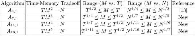
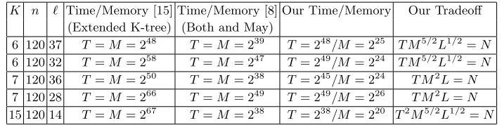
Table 1.Basic List Sum Algorithms
Algorithm Time-Memory Tradeoff Range (M vs.T) Range (M vs.N) Reference
A4,1 T M2=N T1/2 ≤M ≤T N1/4 ≤M ≤N1/3 [13]
A7,1 T M3=N T1/4≤M ≤T1/2 N1/7 ≤M ≤N1/5 New
A11,1 T M4=N T1/7≤M ≤T1/2 N1/11≤M≤N1/6 New
A16,1 T M5=N T1/11≤M ≤T1/2N1/16≤M≤N1/7 New
4.1 Preliminary Construction and Analysis of Basic List Sum Algorithms
Recall that we denote the time complexity of AK by 2τKmfor a parameter τK.
As we show next, the time-memory tradeoff forAK,1is of the formT MαK=N forαK=K−τK.
The basic idea generalizes the one used to constructA4,1in Section 3.4. We deal with an algorithm AK that partitions the problem of size K into several smaller subproblems, solves each one for various choices of intermediate target values and for each such choice, merges the outputs, hopefully obtaining a final solution. When we iterate over a subset that contains a 2−b fraction of the
pos-sible intermediate target values we essentially set an additionalb-bit constraint on the returned solutions. Ideally, this allows to reduce the time complexity of the algorithm by a factor of 2b to 2τKm−b at the expense of nullifying less bits:
recall from (1) that by setting ab-bit constraint on the solutions, we can nullify
n = Km−b−s = Km−b bits (as s = 0 for AK,1). Therefore, we obtain a tradeoff of
T MK−τK =N. (2)
Indeed, after setting theb-bit constraint, we hope to reduce the time complexity to T = 2τKm−b and obtain T MK−τK = 2τKm−b+m(K−τK) = 2Km−b = 2n = N. We stress that this is an ideal formula which cannot always be achieved using a concrete algorithm. We carefully design such algorithms below, aiming to apply the ideal formula to the widest range of parameters possible. This will be relatively simply for symmetric list sum algorithms, but requires deeper insight for asymmetric algorithms.
As deduced above in (2), ideally the tradeoff curve of a basic list sum algo-rithm of typeAK,1 is of the form
T MαK=N (3)
for a constantαK =K−τK. When considering the variant AK,2m, we require
2msolutions and the number of bits that can be nullified is reduced from n to n−m. Consequently, the tradeoff becomesT MαK =N0 forN0= 2n−m, giving
T MαK−1=N. (4)
4.2 Basic Symmetric List Sum Algorithms
The algorithms A4,1 and A4,2m for K = 4 (that are applicable in the range T1/2≤M ≤T) were already constructed in Section 3.4, where we showed that indeedα4= 4−τ4= 2. We continue withK= 16.
A16,1andA16,2m Following the general approach above, we extend the 16-way
list sum algorithmA16 of Section 3.2. Since the time complexity ofA16is 211m, we have τ16 = 11 and α16 = 16−τ16 = 5 as given by (2) and (3). Below, we perform this computation in more detail and calculate the range for which this tradeoff is applicable.
If we fix all the wordsc1, c2, c3, c4inA16(such that their sum is 0), we cast a constraint of 9mbits on the 16-tuples and can nullifyn= 16m−9m= 7mbits in time complexity 22m(which is the time complexity of theA
4algorithms). More generally, when we vary 2v times the value of c
1, c2, c3, c4, we cast a (9m−v)-bit constraint on the 16-tuples and nullifyn= 16m−(9m−v) = 7m+v
bits in time complexityT = 22m+v, giving a tradeoff of
T M5=N,
namelyα16= 5 as expected. Since we can choose any 0≤v≤9m, the tradeoff is applicable for T1/11≤M ≤T1/2.
Beyond 16-Way List Sum Algorithms In order to extend the tradeoff curve ofA4,1to smaller memory ranges ofM ≤T1/2 we squaredK. We can continue to extend the curve to very small memory values in a similar way by defining
AK for K= 162 = 256 and transforming it toAK,1. For even smaller memory ranges, we useK= 2562= 216 and so forth.
4.3 Basic Asymmetric List Sum Algorithms
A7,1 andA7,2m We extend the 7-way dissectionA7of Section 3.3, whose time
complexity is 2τ7m= 24mtoA
7,1. According to the preliminary analysis above, we have α7= 7−τ7= 3, as obtained in more detail below.
If we fix the 2m-bit valuecin the loop ofA7, we set a 2m-bit constraint and can nullify 7m−2m= 5mbits in time 24m−2m= 22m. In general, when we vary
2v times the value ofc, we nullify n= 5m+v bits in timeT = 22m+v, giving
T M3=N,
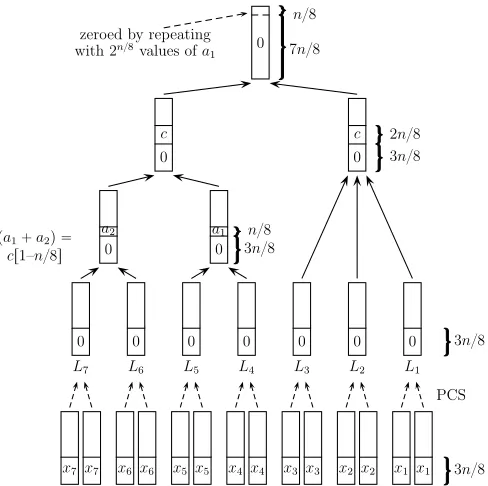
L7 L6 L5 L4 L3 L2 L1
a2
pa1`a2q “
cr1–n{5s a1 n{5
c c 2n{5
0 4n{5
n{5 zeroed by repeating
with 2n{5values ofa
1
1
a1 (along witha2) varies whilecis fixed.
Fig. 1.A7,1 withM = 2n/5, T = 22n/5
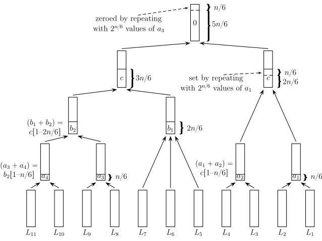
A11,1 and A11,2m We consider the next value of K = 11 in the dissection
sequence described in Section 3.3, which has time complexity of T = 27m
(nul-lifying 11m bits), i.e., τ11 = 7. The main loop of A11 splits the problem into subproblem of sizes 4 and 7, while iterating over 3mintermediate target values. To construct A11,1, we can easily fix these 3m values which reduces the time complexity to 24m (nullifying only 8m bits). In general, we obtain the tradeoff T M4 =N (α11 = 11−τ11 = 4) for T1/7 ≤ M ≤ T1/4. Interestingly, we can recursively fix more values and extend this tradeoff toT1/7≤M ≤T1/2, which is crucial when the number of solutions is large. Below, we describe the algo-rithm for M =T1/2 (i.e.,M = 2n/6, T = 22n/6). This algorithm is sketched in Figure 2.
1. For a fixed 3m-bit word c, apply the A4,2m algorithm to {Li}4i=1 with
the target value c, and store the expected number of 24m−3m = 2m
outputs in a new sorted list L0. Each word is stored along with the corresponding 4-tuple of indexes from{Li}4
i=1.
2. Apply aA7,22m algorithm to{Li}11i=5 with the 3m-bit target valuec by
recursively fixing (additional) 2mbits (the expected number of solutions is indeed 27m−3m−2m= 22m). For each returned solution{yi}11
i=5, look for matches with{yi}4i=1inL0and obtain an 11-tuple{yi}11i=1such that P11
i=1yi= 0 as required.
The complexity of both steps is 22m, henceT = 22m. Altogether, 3m+ 2m= 5m
2n/6, T = 22n/6 as claimed. The ability to recursively fix target values (while maintaining the tradeoff of (3)) is a distinct feature of asymmetric algorithms. Next, we elaborate on which and how many values can be fixed this way for generalK.
L11 L10 L9 L8 L7 L6 L5 L4 L3 L2 L1
a2
pa1`a2q “
cr1–n{6s a1 n{6
a4
pa3`a4q “
b2r1–n{6s a3 n{6
b2 b1 2n{6
pb1`b2q “
cr1–2n{6s
c 3n{6 set by repeating c 2n{n{66
with 2n{6values ofa
1
0 zeroed by repeating
with 2n{6values ofa
3 5n{6
n{6
1
a1 (along witha2) anda3 (along witha4) vary whileb1, b2, care fixed.
Fig. 2.A11,1withM = 2n/6, T = 22n/6
Generic Analysis of Basic Asymmetric List Sum Algorithms We ana-lyze the transformation of the Ki-way dissection algorithmAKi (mentioned in
Section 3.3) to AKi,1. As described in Section 3.3,AKi forKi = 1 +i(i+ 1)/2
runs in time 2τKim for τ
Ki = 1 +i(i−1)/2. Therefore αKi = Ki−τKi = i,
ideally giving the tradeoff
T Mi=N.
Determining the range of parameters for which this tradeoff applies is more subtle, as demonstrated forA11,1above. Recall from Section 3.3 thatAKi splits
the algorithm cannot be reduced below the time complexity of Ai,6 which is
2τim. In conclusion, the tradeoff is applicable in the rangeT1/τKi ≤M ≤T1/τi.
For example, for i = 3, we have K3 = 7, τ7 = 4 (as the time complexity of AK3 = A7 is 24m) and τ3 = 2 (as the time complexity ofAi =A3 is 22m). Therefore, we obtain the tradeoff T M3=N, applicable forT1/4 ≤M ≤T1/2, which indeed coincides with theA7,1tradeoff obtained above. Fori= 4, we have
K4= 11 and obtain the tradeoffT M4=N, applicable forT1/7≤M ≤T1/2. We conclude the analysis with several observations.
– The optimal time complexity in the tradeoff range of basic list sum algo-rithms is determined by the largest subproblem that they solve. Since sym-metric algorithms partition the problem evenly, they have an advantage over asymmetric algorithms in case we are interested only in a small fraction of many solutions (and hence can fix many intermediate target values) and care only about time complexity.
– On the other hand, in many practical GBP instances the number of solutions is limited and asymmetric algorithms may have a significant advantage (as we show in Section 7) by better exploiting the solution space. Moreover, asymmetric algorithms offer substantially better time-memory tradeoffs for many parameters (as demonstrated explicitly in Section 5.3).
– Technically, basic asymmetric list sum algorithms are constructed from ex-haustive algorithms by recursively fixing intermediate target values. The values are fixed in the order of recursion from the largest K value to the smallest until we cannot further improve the time complexity (e.g., forA11,1 we fix values inside the recursive calls with K = 11 and K = 7, but not
K= 4). On the other hand, for symmetric algorithms (such asA16,1), val-ues are fixed in the main loop in an arbitrary manner.
5
Construction of New Multiple-Layer List Sum
Algorithms
The second part of our framework uses the basic AP,1 and AP,2m algorithms
developed in the previous sections in order to construct multi-layered algorithms
AP K.
7The most relevant multi-layer list sum algorithms obtained in this section and in [19] are summarized in Table 2.
The analysis forAP
K will use the parameterαP established forAP,1according to its tradeoff curve (3).
6
We could try to fix additional intermediate target values that the algorithm Ai
iterates over internally. However, this generally results in a less efficient tradeoff compared toT Mi=N.
7
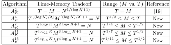
Table 2.Multiple-Layer List Sum Algorithms
Algorithm Time-Memory Tradeoff Range (M vs.T) Reference
A2K T=M =N
1/(logK+1)
T =M [19]
A4
K T
b(logK)/2c
Md(logK)/2e+1
=N T1/2 ≤M ≤T New
A7
K Tlog7KM2 log7K+1=N T1/4≤M ≤T1/2 New A11K T
log11K
M3 log11K+1=N T1/7≤M ≤T1/2 New A16
K Tlog16KM4 log16K+1=N T1/11≤M ≤T1/2 New
5.1 Generic Construction and Analysis of Multiple-Layer Algorithms
We assume that K =Pk ·Q, where 1 ≤Q < P andP, k, Q are integers (if K
is not of the required form we round it down to K0 of this form and apply the algorithm forK0). In this decomposition, we havek= logPK(the logarithm is
rounded down to the nearest integer). We construct the algorithmAPK. IfQ = 1, AP
K hask−1 layers of AP,2m (merging the lists in groups of P,
where each merge outputs a list of 2m inputs into the next layer) and a final
layer ofAP,1. IfQ >1,APK hask layers ofAP,2m and a final layer ofAQ,1.
First, we analyze the case ofK=Pk (namely,Q= 1), based on the tradeoff parameterαP forAP,1 (as specified in (3)). Fix a parameter n0 such that each of the k−1 layers of AP,2m nullifies n0 bits in time complexity 2n
0
−(αP−1)m,
according to the tradeoff curve (4) for AP,2m. Altogether, n0(k−1) bits are
nullified in these layers andn−n0(k−1) remain to be nullified by the final layer
AP,1 in time 2n−n
0(k−1)−α
Pm. In order to balance the algorithm, we equate the
time complexities of the layers by settingn0−(αP−1)m=n−n0(k−1)−αPm
or n0= (n−m)/k. Consequently, the time complexity of the layered algorithm is T = 2n0−(αP−1)m = 2(n−m)/k−(αP−1)m = 2(n−m(k(αP−1)+1))/k. This gives a
time-memory tradeoff ofTkMk(αP−1)+1=N or
TlogPKMlogPK·(αP−1)+1=N. (5)
It is applicable for the same time-memory range asAP,1 (andAP,2m).
For example, in the K-tree algorithm, we haveP = 2 and α2 = 2−τ2 = 1. Hence, the tradeoff of TlogPKMlogPK·(α2−1)+1 collapses to TlogKM = N.
SettingT =M (which is the only point in which the K-tree algorithm is directly applicable) gives the standard formula ofTlogK+1=N orT =N1/(logK+1).
In case K = Pk ·Q for 1 < Q < P, the generic analysis becomes more
involved and depends on the time-memory tradeoff curve ofAQ,1.
In this paper we focus on Q = 2, where the final merge is a basic A2,1 algorithm that runs in fixed time complexity of 2m and nullifies 2m bits. Fix
a parametern0 such that each of thek layers ofAP,2m nullifies n0 bits in time
The algorithm’s time complexity is dominated by the first k layers and is therefore T = 2n0−(αP−1)m = 2(n−2m)/k−(αP−1)m = 2(n−m(k(αP−1)+2))/k. This
gives a time-memory tradeoff of
TlogPKMlogPK·(αP−1)+2=N, (6)
applicable for the same time-memory parameter range asAP,1(andAP,2m).
5.2 Analysis of Specific Multiple-Layer List Sum Algorithms
We analyze the A4K algorithm according to the generic approach above. The analysis of the rest of the layered algorithms APK summarized in Table 2 is obtained in a similar manner by plugging the relevantαP parameter into (5).
A4
K For arity P = 4, we only analyze values of K which are powers of 2 (as
this allows direct comparison to previous tradeoffs for GBP). ForA4,1, we have
α4= 2, established in Section 4.2. In case K = 4k, we plug log
PK = log4K = logK/2 and αP = α4 = 2 into (5), obtaining
T(logK)/2M(logK)/2+1=N,
applicable for T1/2≤M ≤T (as theA
4,1andA4,2m algorithms).
We demonstrate theA4
16 algorithm (that works in two layers) below. 1. Apply the A4,2m algorithm of Section 3.4 four times to lists {Li}4i=1,
{Li}8i=5, {Li}12i=9 and {Li}16i=13, nullifyingn0 = (n−m)/2 bits. Obtain four sorted listsL01, L02, L03, L04, each of expected size 2m.
2. Apply theA4,1algorithm of Section 3.4 toL01, L02, L03, L04, nullifying the remainingn−n0 = (n+m)/2 bits. Derive a single solution to the list sum problemP16
i=1yi[1–n] = 0.
In case K = 2·4k, we have P = 4, Q = 2 and log
4K = (logK −1)/2. Plugging these values into (6) we obtain
T(logK−1)/2M(logK−1)/2+2=N,
applicable for T1/2≤M ≤T.
Unified formula for powers of 2. Unifying the tradeoff formulas obtained above to anyK= 2k, we obtain
Tb(logK)/2cMd(logK)/2e+1=N,
5.3 Comparison of Single-Solution List Sum Algorithms
As shown in Table 2, A16
K is applicable in the range T1/11 ≤M ≤T1/2, while A7
K is applicable in the range T1/4 ≤ M ≤ T1/2. Hence, both algorithms are
applicable inT1/4≤M ≤T1/2 and it is interesting the investigate which of the algorithms is more efficient in this parameter range. The goal of this section is to compare the efficiency single-solution list sum algorithms (such asA16K andA7K) for any fixed value ofK for parameters where the algorithms can be applied.
The efficiency of the algorithms is determined by the tradeoff formula (5). The difficultly in applying this formula to A16
K is that this algorithm is directly
applicable only for values ofKthat are powers of 16. Hence the logarithm log16K is rounded down in (5) forK= 16. Similarly,A7
K is directly applicable only for
values ofKthat are powers of 7.
In general, the difficultly in comparing AP1K andAP2K for a fixed value of K
(for parameters in which both are applicable), is that we need to round down the logarithms logP1Kand logP2Kin (5). To simplify the analysis, we assume that
the tradeoffs are continuous and can be evaluated at any positive real numberK
with no rounding. Hence, we equate the time and memory complexitiesT, M of these algorithms for a fixed valueK=K1= (P1)k1 = (P2)k2=K2and compare the resulting values ofN. We then investigate the implications this comparison.
Continuous analysis. According to (5) the tradeoff forAP
Kis of the formT
logPKMlogPK·(αP−1)+1= N (for a valueαP forAP,1). For a parameterx, letT =Mxbe a point for which
the tradeoff is applicable. Then, we obtain the equalityMxlogPKMlogPK·(αP−1)+1= N orMlogPK(x+αP−1)+1=N. Converting to base 2, the exponent ofM is equal
to logK/logP·(x+αP−1) + 1.
Therefore, in order to compare two tradeoffsTlogP1KMlogP1K·(αP1−1)+1=N
and TlogP2KMlogP2K·(αP2−1)+1=N (for K= (P1)k1 andK = (P
2)k2, respec-tively), we can compare their exponents after plugging inT =Mxfor a value of
xfor which both are applicable. Hence, the tradeoff forAP1
K is superior if and only if
logK/logP1·(x+αP1−1) + 1>logK/logP2·(x+αP2−1) + 1, (7)
or
x >1 + (αP2logP1−αP1logP2)/(logP2−logP1). (8) Note that the last formula does not depend onK.
We say that if the above formulas hold, thenAP1
K isweakly superior toA P2 K
(for the relevant parameter range). Indeed, this does not imply that AP1 K is
actually more efficient than AP2K for a fixed value of K, as we did not round down the logarithms logP1K and logP2K in (5) as required. The consequences
of this comparison are given by the theorem below.
Theorem 1. Assume that AP1K is weakly superior to AP2K in a range of T, M
1. TheAP1K algorithm is more efficient than theAP2K algorithm for all values of
K= (P1)k for an integer k.
2. There exists a value ofK0 such that theAP1
K algorithm is more efficient than
theAP2
K algorithm for anyK > K0 (including K= (P2)k for an integer k). For example, we will show that forT1/4≤M ≤T1/2.7,A7
Kis weakly superior
to A16K. The theorem implies that for T1/4 ≤M ≤T1/2.7, A7K is always more efficient than A16K for values ofK that are powers of 7. Moreover, for T1/4 ≤ M ≤T1/2.7, there exists a value ofK0 such that A7K is more efficient thanA16K
for anyK > K0.
Proof. The first part of the theorem follows from the fact that whenK= (P1)k, the AP1
K algorithm can be directly applied with no rounding loss in logP1K.
Comparing exponents, the left hand side of (7) remains the same forAP1
K, whereas
the right hand side can only decrease for AP2
K due to rounding. As a result, the
value ofN forAP1K remains larger.
The second part of the theorem is obtained by analyzing the efficiency loss due to rounding, and showing that it becomes negligible asKgrows to infinity. From (7) we get 1/logP1·(x+αP1−1)>1/logP2·(x+αP2−1). Therefore,
lim
K→∞logK·(1/logP1·(x+αP1−1)−1/logP2·(x+αP2−1)) =∞.
The rounding loss for AP1
K can decrease the factor logP1K = logK/logP1
in (7) by less than 1. To complete the proof we show that (7) holds for all sufficiently large Keven after this loss, namely, (logK/logP1−1)·(x+αP1− 1) + 1>logK/logP2·(x+αP2−1) + 1. Equivalently,
logK·(1/logP1·(x+αP1−1)−1/logP2·(x+αP2−1))> x+αP1−1,
which holds for all sufficiently largeKas the left hand side approaches infinity, while the right hand side is constant.
We note that the value ofK0 in the second part of the theorem depends on the actual tradeoffs and the value ofxin the proof.
Comparison of Specific Single-Solution List Sum Algorithms Since the tradeoffs ofAPKforP∈ {7,11,16}are applicable in intersecting ranges (as shown in Table 2), we compare their efficiency.
Using (8) by settingP1 = 7 and P2 = 16, we obtain the crossover point of
Table 3.Comparison of List Sum Algorithms
Range Weakly Best Algorithm
T1/2.7≤M ≤T1/2 A16K T1/4≤M ≤T1/2.7 A7
K T1/7≤M≤T1/4 A11
K T1/11≤M ≤T1/7 A16K
6
Construction of New Algorithms for the Generalized
Birthday Problem
The third part of our framework combines preparation phase and list sum al-gorithms (for S = 1) to obtain new GBP algorithms. It combines either PCS (parallel collision search) or CTP (clamping through precomputation) with a given list sum algorithm in a generic manner. The generic formulas are then used to obtain improved tradeoffs for various specific K values (some of which are specified in Table 4). We focus on values ofKthat allow direct comparison to previous tradeoff curves in addition to values that are relevant to Section 7, where we analyze concrete GBP instances.
Table 4.Time-Memory Tradeoffs of GBP Algorithms
K Time-Memory Tradeoff Range (M vs.T) Building Blocks ≥8 Td(logK)/2e+1
Mb(logK)/2c
=N T1/2≤M ≤T PCS +A4
K/2 ≥8T2M3d(logK)/2e−2−(logK) mod 2=N 1≤M ≤T1/2 PCS +A4K/2 8 T3M =N T1/2≤M ≤T PCS +A4,1 8 T2M3=N 1≤M ≤T1/2 PCS +A
4,1 16 T3M2=N T1/2≤M ≤T PCS +A4
8 16 T3M2=N T1/4≤M ≤T1/2 PCS +A7,1 16 T2M6=N 1≤M ≤T1/4 PCS +A
7,1 32 T4M2=N T1/2≤M ≤T PCS +A4
16 32 T3M4=N T1/11≤M ≤T1/2 PCS +A16,1 32 T2M15=N 1≤M ≤T1/11 PCS +A16,1
6 T2M2=N 1≤M ≤T1/2 PCS +A 3,1 7 T2M2=N T1/4≤M ≤T1/2 CTP +A7,1 14 T3M2=N T1/4≤M ≤T1/2 PCS +A7,1 14 T2M6=N 1≤M ≤T1/4 PCS +A
7,1
β, γ. Our analysis also uses a parameterδ, which specifies the lower range limit for the tradeoff algorithm of A as M ≥T1/δ. For example, we established the
tradeoff T M3 = N for A
7,1 in the range T1/4 ≤ M ≤ T1/2, hence we have
β = 1, γ = 3, δ = 4. We will derive a basic tradeoff for M ≥ T1/δ and then
extend it toM < T1/δ. Furthermore, the tradeoffs depend on the input range size L= 2`since the complexity of the preparation phase algorithm varies according
on whether or not`is below some value. For example, when applying PCS with a small value of`, we have to apply it to an expanding function and adapt the complexity as specified on Section 3.6.
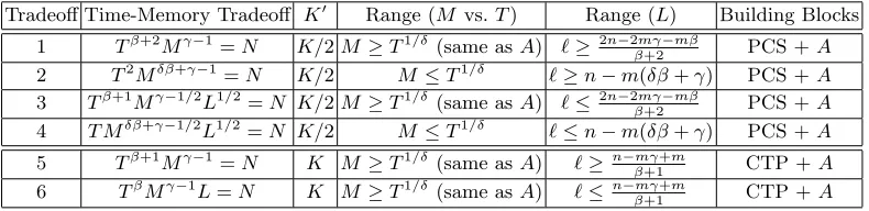
Altogether, a GBP tradeoff formula depends on a triplet of parameters (prepa-ration phase algorithm, memory range, input size range) and there are 23 = 8 such possible triplets. However, we only derive and use 6 of these in this paper, as summarized in Table 5. Due to lack of space, these 6 algorithms and their analysis are described in Appendix D. Below, we explicitly derive the first 4 tradeoffs for the specific case of K= 14 with the PCS preparation phase.
Table 5.Generic GBP Time-Memory Tradeoffs Formulas
Tradeoff Time-Memory Tradeoff K0 Range (M vs.T) Range (L) Building Blocks
1 Tβ+2Mγ−1=N K/2M ≥T1/δ(same asA) `≥2n−2mγ−mβ
β+2 PCS +A 2 T2Mδβ+γ−1
=N K/2 M≤T1/δ `≥n−m(δβ+γ) PCS +A
3 Tβ+1Mγ−1/2L1/2=N K/2M ≥T1/δ(same asA) `≤2n−2mγ−mβ
β+2 PCS +A 4 T Mδβ+γ−1/2L1/2=N K/2 M≤T1/δ `≤n−m(δβ+γ) PCS +A
5 Tβ+1Mγ−1
=N K M≥T1/δ(same asA) `≥n−mγ+m
β+1 CTP +A 6 TβMγ−1L=N K M≥T1/δ(same asA) `≤n−mγ+m
β+1 CTP +A
6.1 Tradeoff Algorithm for K= 14
For K = 14 with the PCS preparation phase, we use an algorithm A for
K0 =K/2 = 7, namely A7,1. The tradeoff formula forA7,1 is T M3 =N (i.e., its time complexity isT = 2n−3m) in the rangeT1/4≤M ≤T1/2. The combi-nation algorithm uses the truncated functionH|r,r (as defined in Section 2) for
a parameterr≥m, set below to optimize the algorithm.
1. Run PCS on the function H|r,r and look for 2m collisions. For each
collisionH(x)[1–r] =H(x0)[1–r], computey=H(x) +H(x0) and store all these words in 7 lists {Li}7i=1 of size about 2m (along with the correspondingxvalues).
2. RunAon{Li}7i=1(nullifying bits [r+1–n]). Obtain 7 wordsyi∈Lisuch
thatP7
solution to GBP by recovering theKwordsxi such thatP
14
i=1H(xi) = P7
i=1yi= 0 as required.
In the first step, we execute PCS with parameter r in time 2(r+m)/2 (ac-cording to Section 3.6). In the second step we nullify the remaining n0 =n−r
bits by using A7,1 in time complexity 2n
0
−3m= 2n−r−3m. Then, to balance the
two steps we require (r+m)/2 =n−r−3mor r= (2n−7m)/3, giving time complexity ofT = 2(n−2m)/3 and a tradeoff of
T3M2=N.
This matches Tradeoff 1 forK= 14 in Table 5 (recall that forA7,1, β= 1, γ= 3, δ= 4). This tradeoff is valid forT1/4≤M ≤T1/2(asA
7,1). The algorithm for parameters T =N1/4, M =N1/8 (which improves upon the K-tree algorithm) is sketched in Figure 3.
WhenM < T1/4, we can extend the tradeoff by applyingA
7,1to nullify less bits (i.e., with a smaller value of n0), implying that PCS will nullify more bits and dominate the complexity of the algorithm which becomesT = 2(r+m)/2= 2(n−n0+m)/2
. In order to calculaten0, we use the tradeoff curve ˆT M3=N0ofA7,1 at its lower range M = ˆT1/4 or ˆT =M4 (here, ˆT denotes the time complexity of A7,1) and obtainN0 =M7, namely n0 = 7m. Therefore, T = 2(n−n
0+m)/2
= (n−6m)/2, giving the tradeoff
T2M6=N.
This matches Tradeoff 2 in Table 5.
Restricted Domain Recall from the first tradeoff that r = (2n−7m)/3. In case ` < r = (2n−7m)/3 (the domain size of H is 2` <2r) we are forced to
use H|`,r which is an expanding function. The time complexity of PCS for the
expanding function H|`,r is 2r+(m−`)/2 (as specified in Section 3.6), while the
time complexity ofA7,1 remainsT = 2n−r−3m. Balancing the steps in this case givesr+ (m−`)/2 =n−r−3morr=n/2−7m/4 +`/4 and time complexity ofT =r+ (m−`)/2 =n/2−5m/4−`/4. This gives the formula
T2M5/2L1/2=N,
matching Tradeoff 3 in Table 5.
WhenM < T1/4, the steps cannot be balanced as above and the time com-plexity becomes 2r+(m−`)/2 (dominated by PCS). Here, r= n−n0 = n−7m (n0 = 7m as in the case where the domain is not restricted). We obtain T = 2n−13m/2−`/2, giving the formula
T M13/2L1/2=N
x7 x7 x6 x6 x5 x5 x4 x4 x3 x3 x2 x2 x1 x1 3n{8
PCS
L7
0
L6
0
L5
0
L4
0
L3
0
L2
0
L1
0 3n{8
0
a2
pa1`a2q “
cr1–n{8s 0 a1
3n{8
n{8 0
c
0
c
3n{8
2n{8
0 7n{8
n{8 zeroed by repeating
with 2n{8values ofa
1
1
a1 (along witha2) varies whilecis fixed. PCS colliding values (xi’s) are arbitrary.
Fig. 3.GBP Algorithm forK= 14 withM= 2n/8, T = 2n/4
6.2 Tradeoff Formulas for K= 2k (andK ≥8)
We now derive improved GBP tradeoffs forK= 2kassuming thatK≥8. These
tradeoffs are obtained by combining PCS with multiple layers of the 4-way list sum algorithm A4
K/2 (described in Section 5) as the generic algorithm A. The formula is calculated according to Tradeoff 1 in Table 5.
We recall the formula ofA4K/2from Table 2, which isTb(logK−1)/2cMd(logK−1)/2e+1=
N,8namelyβ=b(logK−1)/2c=d(logK)/2e−1 andγ=d(logK−1)/2e+1 = b(logK)/2c+ 1. Adding 2 toβand reducingγby 1 (as in Tradeoff 1 in Table 5), we obtain
Td(logK)/2e+1Mb(logK)/2c =N,
applicable for T1/2≤M ≤T.
Extending the Tradeoffs to M < T1/2 In case M < T1/2, PCS dominates the algorithm’s time complexity and the formula is given in Tradeoff 2 in Table 5
8