Poly-Logarithmic Side Channel Rank Estimation
via Exponential Sampling
Liron David1, Avishai Wool2
School of Electrical Engineering, Tel Aviv University, Ramat Aviv 69978, Israel 1
[email protected],[email protected]
Abstract. Rank estimation is an important tool for a side-channel eval-uations laboratories. It allows estimating the remaining security after an attack has been performed, quantified as the time complexity and the memory consumption required to brute force the key given the leakages as probability distributions over d subkeys (usually key bytes). These estimations are particularly useful where the key is not reachable with exhaustive search.
We propose ESrank, the first rank estimation algorithm that enjoys prov-able poly-logarithmic time- and space-complexity, which also achieves excellent practical performance. Our main idea is to use exponential sampling to drastically reduce the algorithm’s complexity. Importantly, ESrank is simple to build from scratch, and requires no algorithmic tools beyond a sorting function. After rigorously bounding the accuracy, time and space complexities, we evaluated the performance of ESrank on a real SCA data corpus, and compared it to the currently-best histogram-based algorithm. We show that ESrank gives excellent rank estimation (with roughly a 1-bit margin between lower and upper bounds), with a performance that is on-par with the Histogram algorithm: a run-time of under 1 second on a standard laptop using 6.5 MB RAM.
1
Introduction
1.1 Background
Side-channel attacks (SCA) represent a serious threat to the security of crypto-graphic hardware products. As such, they reveal the secret key of a cryptosystem based on leakage information gained from physical implementation of the cryp-tosystem on different devices. Information provided by sources such as timing [12], power consumption [11], electromagnetic emulation [21], electromagnetic radiation [2, 9] and other sources, can be exploited by SCA to break cryptosys-tems.
set of popular attacks, and to determine whether the adversary can break the implementation (i.e., recover the key) using “reasonable“ efforts.
Most of the attacks that have been published in the literature are based on a “divide-and-conquer” strategy. In the first “divide” part, the cryptanalyst recov-ers multi-dimensional information about different parts of the key, usually called subkeys (e.g., each of the d= 16AES key bytes can be a subkey). In the “con-quer” part the cryptanalyst combines the information all together in an efficient way via key enumeration [19, 23, 6]. In the attacks we consider in this paper, the information that the SCA provides for each subkey is a probability distribution over the N candidate values for that subkey, and the SCA probability of a full key is the product of the SCA probabilities of itsdsubkeys.
A security evaluator knows the secret key and aims to estimate the number of decryption attempts the attacker needs to do before he reaches to the cor-rect key, assuming the attacker uses the SCA’s probability distribution. Clearly enumerating the keys in the optimal SCA-predicted order is the best strategy the evaluator can follow. However, this is limited by the computational power of the evaluator. This is a worrying situation because it is hard to decide whether an implementation is “practically secure”. For example, one could enumerate the
250first keys for an AES implementation (in the optimal order) without finding the correct key, and then conclude that the implementation is practically secure because the attacker needs to enumerate beyond250 number of keys. But, this does not provide any hint whether the concrete security level is251or2120. This makes a significant difference in practice, especially in view of the possibility of improved measurement setups, signal processing, information extraction, etc., that should be taken into account for any physical security evaluation, e.g., via larger security margins.
In this paper, we introduce a new method to estimate the rank of a given secret key in the optimal SCA-predicted order. Our algorithm enjoys simplicity, accuracy and provable poly-logarithmic time and memory efficiency and excellent practical performance.
The rank estimation problem: Givend independent subkey spaces each of sizeN with their corresponding probability distributionsP1, ..., Pd such thatPi
is sorted in decreasing order of probabilities, and given a key k∗ indexed by
(k1, ..., kd), letp∗=P1(k1)·P2(k2)·...·Pd(kd)be the probability ofk∗to be the correct key. The evaluator would like to estimate the number of full keys with probability higher than p∗, when the probability of a full key is defined as the product of its subkey’s probabilities.
In other words, the evaluator would like to estimatek∗’s rank: the position of the key k∗ in the sorted list of Nd possible keys when the list is sorted
fast and low-memory algorithms to estimate the rank without enumeration is of great interest.
1.2 Related work
The best key enumeration algorithm so far, in terms of optimal-order, was pre-sented by Veyrat-Charvillon, Gérard, Renauld and Standaert in [23]. However, its worst case space complexity is Ω(Nd/2) when d is the number of subkey dimensions andN is the number of candidates per subkey - and its space com-plexity isΩ(r)when enumerating up to a key at rank r≤Nd/2. Thus its space complexity becomes a bottleneck on real computers with bounded RAM in re-alistic SCA attacks.
Since then several near-optimal key enumeration were proposed [4, 18, 20, 26, 3, 10, 6, 15, 13, 14, 17, 22]. However, none of these key enumeration algorithms enumerate the whole key space within a realistic amount of time and with a realistic amount of computational power: enumerating an exponential key space will always come at an exponential cost. Hence the need for efficient and accurate rank estimation for keys that have a high rank.
The first rank estimation algorithm was proposed by Veyrat-Charvillon et al. [24]. They suggested to organize the keys by sorting their subkeys accord-ing to the a-posteriori probabilities provided, and to represent them as a high-dimensional dataspace. The full key space can then be partitioned in two vol-umes: one defined by the key candidates with probability higher than the correct key, one defined by the key candidates with probability lower than the correct key. Using this geometrical representation, the rank estimation problem can be stated as the one of finding bounds on these “higher” and “lower” volumes. It essentially works by carving volumes representing key candidates on each side of their boundary, progressively refining the lower and upper bounds on the key rank. Refining the bounds becomes exponentially difficult at some point.
A number of works have investigated solutions to improve upon [24]. In par-ticular, Glowacz et al. [10] presented a rank estimation algorithm that is based on a convolution of histograms and allows obtaining tight bounds for the key rank of (even large) keys. This Histogram algorithm is currently the best rank estimation algorithm we are aware of. The space complexity of this algorithm is O(dB)where dis the number of dimensions and B is a design parameter con-trolling the number of the histogram bins. A comparable result was developed independently by Bernstein et al. [3].
Ye et al. investigated an alternative solution based on a weak Maximum Likelihood (wML) approach [26], rather than a Maximum Likelihood (ML) one for the previous examples. They additionally combined this wML approach with the possibility to approximate the security of an implementation based on “easier to sample” metrics, e.g., starting from the subkey Success Rates (SR) rather than their likelihoods. Later Duc et al. [7] described a simple alternative to the algorithm of Ye et al. and provided an “even easier to sample” bound on the subkey SR, by exploiting their formal connection with a Mutual Information metric. Recently, Wang at al. [25] presented a rank estimation for at dependent score lists.
Choudary et al. [5] presented a method for estimating Massey’s guessing entropy (GM) which is the statistical expectation of the position of the correct key in the sorted distribution. Their method allows to estimate the GM within a few bits. However, theactualguessing entropy (GE), i.e., therankof the correct key, is sometimes quite different from the expectation. In contrast, our algorithm focuses on the real GE.
1.3 Contribution
In this paper we propose a simple and effective new rank estimation method called ESrank, that is fundamentally different from previous approaches. We have rigorously analyzed its accuracy, time and space complexities. Our main idea is to use exponential sampling to drastically reduce the algorithm’s com-plexity. We prove ESrank has a poly-logarithmic time- and space-complexity: for a design parameter 1< γ <2 ESrank hasO(d42(logγN)2log(log
γN))time
andO(dlogγN+d2
16(logγN)2)space, and it can be driven to any desired level of
accuracy (trading off time and space against accuracy). Importantly, ESrank is simple to build from scratch, and requires no algorithmic tools beyond a sorting function.
Beyond asymptotic analysis, we evaluated the performance of ESrank through extensive simulations based on a real SCA data corpus, and compared it to the currently-best histogram-based algorithm. We showed that ESrank gives excel-lent rank estimation (with roughly a 1-bit margin between lower and upper bounds), with a performance that is on-par with the Histogram algorithm: a run-time of under 1 second, for all ranks up to2128, on a standard laptop using at most 6.5 MB RAM. Hence ESrank is a useful addition to the SCA evaluator’s toolbox.
2
The ESrank Algorithm for the case
d
= 2
Algorithm 1: Exact rank.
Input:Two non-decreasing probability distributionsP1, P2of sizeN each, the
correct keyk∗= (k1, k2)and its probabilityp∗=P1[k1]·P2[k2].
Output:Rank(k∗).
1 i= 1; j=N; rank= 0;
2 whilei≤N andj≥1do
3 p=P1[i]·P2[j];
4 if p≥p∗then
5 rank=rank+j;
6 i=i+ 1;
7 else
8 j=j−1;
9 returnrank;
2.1 An exact rank estimation for d= 2
Definition 1 (Rank(k∗)). Letdnon-increasing subkey probability distributions Pi for1≤i≤dand the correct key k∗ = (k1, ..., kd)be given. Letp∗=P1[k1]· ...·Pd[kd] be the probability of the correct key. Then, defineRank(k∗)to be the
number of keys(x1, ..., xd)s.t.P1[x1]·...·Pd[xd]≥p∗.
Definition 2. Let 2 non-increasing subkey probability distributions P1 andP2, each of sizeN, the correct key k∗ = (k1, k2) and an index1 ≤i≤N be given. Let p∗ =P1[k1]·P2[k2] be the probability of the correct key. Then define Hi to
be the number of points(i, j)such thatP1[i]·P2[j]≥p∗, i.e.,
Hi(k∗) =|{(i, j)|P1[i]·P2[j]≥p∗}|.
The idea of the algorithm is to findHi(k∗)for eachi. The rank of the correct
keyk∗ is the sum of Hi(k∗)over1≤i≤N, i.e.,
Rank(k∗) = N ∑
i=1
Hi(k∗).
The pseudo code is described in Algorithm 1. The correctness of Algorithm 1 stems from the observation that Hi≥Hi+1 for all1≤i≤N−1. Therefore, to findHi+1,j starts fromHi and it is decreased untilHi+1 is found.
Proposition 1. The running time of Algorithm 1 isΘ(N).
Proof: At the beginningi= 1andj=N. In each iteration eitheriis increased by 1 or j is decreased by 1 until either i = N + 1 or j = 0. Therefore, the number of steps is at most2·N in case both iand j reach their limits, and is at leastN in case only one of them reaches it limit. Therefore, the running time
2.2 Exponential Sampling with d= 2
To make this algorithm faster, we use sampling. Intuitively, we sample a set of indices SI and run Algorithm 1 on the SI×SI grid. On the sampled indices Algorithm 1 is no longer exact, but we can modify it to produce lower and upper bounds onRank(k∗). As we shall see, if we use exponential sampling, defined in Section 2.3, we can bound the inaccuracy introduced by the sampling.
Given a non-increasing subkey probability distributionP of sizeN, the sam-pling process returns a sampled probability distribution (SI, SP) of size Ns
where Ns =O(logN). SI contains the sampled indices andSP contains their
corresponding probabilities such thatSP[i] =P[SI[i]]for alli≤Ns.
The goal of the exponential sampling is to maintain an invariant on the ratio between sampled indices. Let1< γ≤2be given and letbbe the smallestisuch that i/(i−1)≤γ. The firstbsampled indices are the first b indices ofP. The rest of the sampled indices are sampled fromP at powers ofγ. More formally, for alli≤Ns−1 the sampled indices obey:
{
SI[i] =i ifi≤b
SI[i]/SI[i−1]≤γandSI[i+ 1]/SI[i−1]> γ otherwise. (1)
E.g., ifγ= 2thenb= 2, and forSI={1,2,4,8, . . . , N}invariant (1) holds. The pseudo code of this sampling is described in Algorithm 2. Note that the indices 1 andN are always included inSI.
Lemma 1. If SI is the output of Algorithm 2 then for any indexi≥b+ 1 in SI it holds that
SI[i] =⌊γ·SI[i−1]⌋.
and
SI[i]−SI[i−1] =⌊(γ−1)·SI[i−1]⌋.
Proof: According to Algorithm 2, it holds that
SI[i]
SI[i−1] ≤γ
and
SI[i] + 1
SI[i−1] > γ.
Therefore,
γ·SI[i−1]−1< SI[i]≤γ·SI[i−1].
SinceSI[i]is an integer it holds
SI[i] =⌊γ·SI[i−1]⌋.
The differenceSI[i]−SI[i−1]obeys
Algorithm 2: Sampling Process.
Input:A probability distributionP of sizeN,b,γ. Output:A sampled probability distribution(SI, SP).
1 fori= 1 tobdo
2 SI[i] =i; SP[i] =P[i];
3 j=b; i=j+ 1; c=j+ 1;
4 whilei < N do
5 if i/j≤γ and(i+ 1)/j > γ then 6 SI[c] =i; SP[c] =P[i];
7 c=c+ 1; j=i; i=i+ 1;
8 SI[c] =N; SP[c] =P[N];
9 return(SI, SP);
The indices ofSI are integers, therefore we get
SI[i]−SI[i−1] =⌊(γ−1)·SI[i−1]⌋.
⊓ ⊔ Proposition 2. Let Ns=|SI|be the size the sample returned by Algorithm 2.
Thenb+ logγ(N/b)≤Ns< b+ logγ(N/(b−1)).
Proof: Sinceb·rN s≥N andb·rN s−1< N.
Definition 3. Let two sampled probability distributions (SI, SP1),(SI, SP2), each of size Ns, the correct key k∗ = (k1, k2), its probability p∗ and an index
1 ≤ i ≤ Ns be given. Then define HiS to be the number of points (i, j) s.t. 1≤j≤N andSP1[i]·P2[j]≥p∗, i.e.,
HiS(k∗) =|{(i, j)|1≤j≤N andSP1[i]·P2[j]≥p∗}|.
The difference between every two successive indices in the sampled proba-bility distributions might be bigger than 1, i.e.,SI[i+ 1]−SI[i]>1 therefore, besides counting HiS for eachi≤Nswe also need to add the number of points (i, j)such that SI[i] ≤i≤SI[i+ 1]. Recall that Algorithm 2 always includes i=N inSI.
Definition 4. Let two sampled probability distributions (SI, SP1),(SI, SP2), each of size Ns, the correct key k∗ = (k1, k2), its probability p∗ and an index
1 ≤i ≤Ns be given. Then define Ha,bS be the number of (i, j) s.t. 1 ≤j ≤N
andSI[a]< i < SI[b] andSP1[i]·P2[j]≥p∗, i.e.,
Ha,bS (k∗) =|{(i, j)|1≤j ≤N andSP1[i]·P2[j]≥p∗ andSI[a]< i < SI[b]}|.
The idea of Algorithm 3 is to find HS
i(k∗) for each i ∈ {1, ..., Ns} and
HS
i,i+1(k∗) for each i ∈ {1, ..., Ns−1}. The rank of the correct key k∗ is the
following sum:
Rank(k∗) = Ns
∑
i=1
HiS(k∗) + N∑s−1
i=1
Algorithm 3: Calculating Upper and Lower bounds.
Input:Sampled probability distributionsSP1,SP2each of sizeNs,b, the
correct keyk∗= (k1, k2)and it probabilityp∗.
Output:Upper and lower bounds onRank(k∗).
1 iLast=Ns; jLast=Ns;
2 if k1== 1thenjLast=k2;
3 if k2== 1theniLast=k1;
4 i= 1; j=jLast; ub= 0; lb= 0; 5 whilei≤iLastandj≥1do
6 pCurr=SP1[i]·SP2[j];
7 if pCurr≥p∗then
8 u=l=SI2[j]; uP rev=u;
9 ub=ub+u; lb=lb+l;
10 if i≥b+ 1then
11 ub=ub+uP rev·(SI[i]−SI[i−1]−1);
12 lb=lb+l·(SI[i]−SI[i−1]−1);
13 i=i+ 1;
14 else if j >1then
15 pN ext=SP1[i]·SP2[j−1];
16 if pN ext < p∗< pCurr then
17 u=SI[j]−1; l=SI[j−1]; uP rev=u;
18 ub=ub+u; lb=lb+l;
19 if i≥b+ 1then
20 ub=ub+uP rev·(SI[i]−SI[i−1]−1); 21 lb=lb+l·(SI[i]−SI[i−1]−1);
22 i=i+ 1;
23 else
24 j=j−1;
25 else
26 j=j−1;
27 if j <1andi≤iLastthen
28 ub=ub+uP rev·(SI[i]−SI[i−1]−1);
29 return(lb, ub);
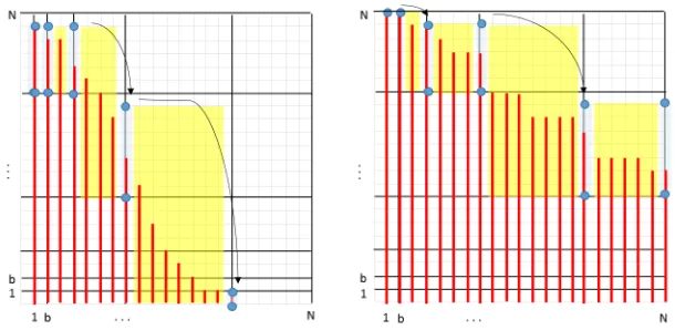
Since we are given sampled distributions, we cannot calculate the exact values ofHS
i (k∗)andHi,iS+1(k∗). Instead we calculate upper and lower bounds for each HS
i(k∗)andHi,iS+1(k∗)as illustrated in Figure 1.
Definition 5. Letup(HS
i (k∗))be an upper bound ofHiS(k∗)and letup(Hi,iS+1(k∗)) be an upper bound of HS
i,i+1(k∗), i.e.,
HiS(k∗)≤up(HiS(k∗))andHi,iS+1(k∗)≤up(Hi,iS+1(k∗)).
Definition 6. Letlow(HiS(k∗))be a lower bound ofHiS(k∗)and letlow(Hi,iS+1(k∗))
be a lower bound ofHi,iS+1(k∗), i.e.,
Fig. 1.The red bars represent the un-sampledHi’s, and the black grid represents the
sampled indices inSI. For each sampled index 1≤i≤Ns the blue circles are upper
and lower bounds on HiS(k∗). The yellow-shaded rectangles representHi,iS+1(k∗) for
eachb≤i≤Ns−1, for two different keys. Note that the yellow-shaded rectangles stop
exactly one index before the sampled indices, in both dimensions.
Therefore, it holds
Ns
∑
i=1
low(Hi(k∗)) + N∑s−1
i=1
low(Hi,i+1(k∗))≤Rank(k∗)≤
≤ Ns
∑
i=1
up(Hi(k∗)) + N∑s−1
i=1
up(Hi,i+1(k∗)).
(2)
2.3 Bounding the Sampled Distributions
Given two probability distributionsP1andP2, each of sizeN, we first sample the indices using Algorithm 2. We get sampled probability distributions (SI, SP1) and(SI, SP2)each of sizeNswhenSIis the set of sampled indices andSP1, SP2 are the corresponding sampled probabilities. Given these sampled probability distributions, the next step is to calculate an upper bound and a lower bound forRank(k∗). This is done in Algorithm 3.
To do this, it keeps two variables:ubfor the upper bound andlbfor the lower bound. At the beginning, both ubandlbare initialized to 0.
Definition 7. Given a keyk∗, and given1≤i≤Ns, letui be the value ofuat
iterationiin Algorithm 3 and letli be the value oflat iterationiin Algorithm 3.
Algorithm 3 starts withi= 1andj =Ns. It decreasesjuntil one of the two
options happens:
(a) (line 16) We reach the highestj such that
In this case (i, j)∈HS
i (k∗)but (i, j−1)∈/HiS(k∗), therefore
SI[j−1]≤HiS(k∗)≤SI[j]−1.
Therefore the values ofli andui become
li=SI[j−1]andui=SI[j]−1, (3)
and the running totalsubandlbare updated (line 9). (b) (line 7) We reach the highestj such that
SP1[i]·SP2[j]≥p∗.
In this case we have the exact value ofHS
i (k∗)which is
HiS(k∗) =SI[j].
Therefore the values ofli andui become
li=ui =SI[j], (4)
and the running totalsubandlbare updated (line 18). In the next step, after finding bounds onHS
i , the algorithm moves toi+1and
finds bounds onHS
i+1. SinceHiS ≥HiS+1we start fromjof the previous iteration i.e.,js.t.SI[j−1]≤HS
i ≤SI[j]and decrease it to get the corresponding bounds
onHS i+1.
Once i≥ b+ 1 (lines 10, 19) the difference SI[i]−SI[i−1]≥ 1 therefore HS
i−1,i(k∗)≥1and it should be added. To upper bound this number we multiply
the upper bound ofHS
i−1, which isuP revi=ui−1, by the width ofHiS−1,i(k∗),
which is (SI[i]−SI[i−1]−1) (lines 11, 20). To lower bound HS
i−1,i(k∗) we
multiply the lower bound ofHS
i , which is li by the width of HiS−1,i(k∗), (lines
12, 21); see Figure 1.
Theorem 1. Let two sampled probability distributionsSP1andSP2, which are sampled from the probability distributions P1 and P2 respectively using Algo-rithm 2 with γ >1 be given and let b be the smallest i such that i/(i−1)≤γ. For a keyk∗, letub andlbbe the outputs of Algorithm 3. Thenub/lb≤γ2.
Proof: From Equation (2) it holds that
ub= Ns
∑
i=1
up(Hi(k∗)) + N∑s−1
i=1
up(Hi,i+1(k∗)).
Since
up(HiS(k∗)) =ui andup(Hi,i+1(k∗)) =ui·(SI[i+ 1]−SI[i]−1)
we get
ub= Ns
∑
i=1 ui+
N∑s−1
i=1
Since SI[i+ 1]−SI[i] = 1for all 1≤i≤b−1, the firstb−1 elements of the second sum are 0.
ub= Ns
∑
i=1 ui+
N∑s−1
i=b
ui·(SI[i+ 1]−SI[i])−1)
b−1
∑
i=1 ui+
N∑s−1
i=b (
ui+ui·(SI[i+ 1]−SI[i]−1) )
+uNs
b−1
∑
i=1 ui+
N∑s−1
i=b
ui·(SI[i+ 1]−SI[i])) +uNs
Separating the b’th term from the second sum we get
ub≤
(∑b−1
i=1 ui
)
+ub·(SI[b+ 1]−SI[b]) +uNs+
N∑s−1
i=b+1
ui·(SI[i+ 1]−SI[i]). (5)
Similarly from Equation (2) it holds that
lb= Ns
∑
i=1
low(Hi(k∗)) + N∑s−1
i=1
low(Hi,i+1(k∗)).
Since
low(HiS(k∗)) =li andlow(Hi,i+1(k∗)) =li+1·(SI[i+ 1]−SI[i]−1)
(Note the shift in indices where the multiplication is by the lower bound ofi+ 1) we get
lb= Ns
∑
i=1 li+
N∑s−1
i=1
li+1·(SI[i+ 1]−SI[i]−1).
Again the firstb−1elements of the second sum are 0, therefore
lb= Ns
∑
i=1 li+
N∑s−1
i=b
li+1·(SI[i+ 1]−SI[i]−1).
By shifting indexi by 1 in the second sum, we get
lb= Ns
∑
i=1 li+
Ns
∑
i=b+1
li·(SI[i]−SI[i−1]−1)
= b ∑
i=1 li+
Ns
∑
i=b+1
(
li+li·(SI[i]−SI[i−1]−1) )
= b ∑
i=1 li+
Ns
∑
i=b+1
li·(SI[i]−SI[i−1])
≥ b ∑
i=1 li+
N∑s−1
i=b+1
li·(SI1[i]−SI1[i−1]).
In order to show ub/lb ≤ γ2, we prove the following two Lemmas (in the Appendix):
Lemma 2. (N∑s−1
i=b+1
ui·(SI[i+ 1]−SI[i]) )
/
(N∑s−1
i=b+1
li·(SI[i]−SI[i−1]) )
≤γ2
Lemma 3. ((∑b−1
i=1 ui
)
+ub·(SI[b+ 1]−SI[b]) +uNs
)
/
(∑b
i=1 li
) ≤γ2.
3
The general case
d >
2
Given d > 2 sampled probability distributions (SI1, SP1), ...,(SId, SPd), and
the correct key k∗ = (k1, ..., kd), we now follow the intuition of thed= 2 case to solve the general case. To do so, we organize the d distributions into pairs, merge the pairs intod/2 joint distributions, sub-sample the joint distributions, and continue in the same way until we get to a single pair of distributions sampled from the Nd/2-dimensioned half-keys. We achieve this via a sequence of algorithms described below.
3.1 Merging two sampled distributions into a joint distribution
Given two sampled non-increasing probability distributions(SI1, SP1),(SI2, SP2), each of sizeNs, we wish to merge them into one non-increasing distribution, and
compute lower and upper bounds on the ranks of the points. Algorithm 4 im-plements this task.
First, the algorithm goes over the grid ofN2
spoints(i, j)such that1≤i≤Ns
and1≤j≤Ns. For each point(i, j)it calculates the point’s probabilitySP1[i]· SP2[j]. Then, we sort these points in decreasing order of their probabilities.
Given two consecutive points (i1, j1) and (i2, j2) in the sorted order such thatP rob(i1, j1)≥P rob(i2, j2), all the points whose probability is greater than P rob(i1, j1) are also greater than P rob(i2, j2), therefore, all the points in the rank of(i1, j1)are contained in the rank of(i2, j2). Relying on this observation, if we know the order of the Ns2 points according to their probabilities, we can bound the accumulative rank of these points while going over them from the most likely point to the least. In this way, the upper-bound of the rank of the current point (ic, jc)is the upper bound of the previous point (ip, jp) plus the
following expressions:
+ (SI[jp+ 1]−SI[jp])·(SI[ip+ 1]−SI[ip]−1)
+SI[jp+ 1]−SI[jp]−1
+ 1
= (SI[jp+ 1]−SI[jp])·(SI[ip+ 1]−SI[ip]).
Algorithm 4: Calculating the joint probability distribution. Input:Sampled probability distributionsSP1,SP2each of sizeNs.
Output:Joint probability distribution.
1 r= 1;
2 fori= 1 toNs do
3 forj= 1toNsdo
4 Y(r,1) =SP1[i]·SP2[j]; Y(r,2) = (i, j);
5 r=r+ 1;
6 Y =Sort(Y)in decreasing order ofY(r,1);
7 ub(1,1) = 1; ub(1,2) =SP1[1]·SP2[1];
8 lb(1,1) = 1; lb(1,2) =SP1[1]·SP2[1];
9 forr= 2toNs2do
10 (ic, jc) =Y(r,2); (ip, jp) =Y(r−1,2);
11 ub(r,1) =ub(r−1,1) + (SI(jp+ 1)−SI(jp))·(SI(ip+ 1)−SI(ip);
12 lb(r,1) =lb(r−1,1) + (SI(jc)−SI(jc−1))·(SI(ic)−SI1(ic−1);
13 ub(r,2) =lb(r,2) =Y(r,2);
14 return(ub, lb);
The first term in (7),(SI[jp+ 1]−SI[jp])·(SI[ip+ 1]−SI[ip]−1), represents
the number of points that might come after the previous point and before the current point, which are not on theSI grid. I.e., these are the points(i, j)s.t.
SI[ip]< i < SI[ip+ 1]and SI[jp]≤j < SI[jp+ 1].
SI[jp+ 1]is not included since we haven’t reached that point yet.
The second term in (7), SI[jp+ 1]−SI[jp]−1, represents the number of
points that might come after the previous point and before the current point whichare on the SIgrid. I.e., these are the points(i, j)s.t.
i=SI[ip] andSI[jp]< j < SI[jp+ 1].
SI[jp] is not included since the point (SI[ip], SI[jp]) is the previous point and
it was already included andSI[jp+ 1]is not included since we haven’t reached
that point yet.
The last addition in (7) is1, accounting for the current point itself.
The resulting expression can be seen in Algorithm 4 (line 11). A similar derivation can be done for the lower bound (omitted).
Note that Algorithm 4 does not require the one-dimensional ranks or even knowing upper or lower bounds on the one-dimensional ranks.
3.2 Sampling the joint probability distribution
The output of Algorithm 4 is a distribution over N2
s elements. We now show
Algorithm 5: Sub-Sampling the joint distribution.
Input:A joint probability distribution(inSI, inSP)of sizeNs2,b,γ.
Output:A sampled probability distribution(SI, SP).
1 fori= 1 tobdo
2 SI[i] =inSI[i]; SP[i] =inSP[i];
3 j=b; i=j+ 1; c=i+ 1;
4 whilei < N2 s do
5 if inSI[i]/inSI[j]≤γandinSI[i+ 1]/inSI[j]> γthen
6 SI[c] =inSI[i]; SP[c] =inSP[i];
7 c=c+ 1; j=i; 8 SI[c] =inSI[N2
s]; SP[c] =inSP[Ns2];
9 return(SI, SP);
We would like to sample this joint probability distribution using Algorithm 2, using b and γ, except now instead of the 1-dimensional ranks we sample using the rank-upper/lower-bounds, See Algorithm 5.
For this, we shall prove in Lemma 5 that the first b indices of the joint probability distribution are 1, ..., b and we shall prove in Theorem 2 that the ratio between any two successive ranks is at mostγ.
Lemma 4. For any indexi≥b+ 1 inSI it holds that
SI[i]−SI[i−1]≤(γ−1)·SI[i−1].
Lemma 5. Given two sampled probability distributions(SI1, SP1)and(SI2, SP2) that are sampled by Algorithm 2 merged by Algorithm 4. The firstb upper ranks in the upper joint probability distribution are the integers 1, .., b and the first b lower ranks in the lower joint probability distribution are the integers1, .., b.
Proof: According to the sampling process in Algorithm 2 it holds: ∀i ≤ b SI1[i] =iandSI2[i] =i. Therefore, the joint probability contains the indices of
(i, j)∈ {1, ..., b} × {1, ..., b}. Since the first bpoints with the highest probabili-ties are somewhere in the square: {1, ..., b} × {1, ..., b} . The rank of the firstb composed only from points in this square, therefore fori≤b, the upper bound and lower bound of the i’th element in the joint distribution are equal to each other and equal toi.
Theorem 2. Given the joint probability distribution of the sampled probability distributions(SI1, SP1),(SI2, SP2), The ratio between any two consecutive upper (lower) ranks is at mostγ, where1< γ≤2.
Proof: Let up(ic, jc) be the upper bound on the rank of point (ic, jc) as in
Algorithm 4. As can be seen in Algorithm 4 the difference between the upper ranks of any two consecutive points(ic, jc)and(ip, jp)is
By Lemma 4 it holds that
SI2(jp+ 1)−SI2(jp)≤SI2(jp)·(γ−1)
SI1(ip+ 1)−SI1(ip)≤SI1(ip)·(γ−1).
Therefore,
up(ic, jc)−up(ip, jp)≤SI2(jp)·SI1(ip)·(γ−1)2
The trivial lower bound ofrank(ip, jp)is the multiplication of its index, therefore
up(in, jn)−up(ip, jp)≤up(ip, jp)·(γ−1)2
Since1< γ≤2, it holds(γ−1)2≤(γ−1), therefore
up(ic, jc)−up(ip, jp)≤up(ip, jp)·(γ−1)
and we get
up(ic, jc)≤up(ip, jp)·γ.
Similarly, as can be seen in Algorithm 4 the difference between the lower ranks of any two successive points(in, jn)and (ip, jp)is
up(ic, jc)−up(ip, jp) = (SI2(jc)−SI2(jc−1))·(SI1(ic)−SI1(ic−1)).
A similar argument shows that low(ic, jc)≤low(ip, jp)·γ.
Theorem 2 shows that in the jointNs×Ns distribution, the upper (lower)
bounds of every two consecutive points (in sorted order) obey the invariant ub(ic, jc)≤γ·ub(ip, jp).
Corollary 1. The sample produced by Algorithm 5 on an input distribution of sizeN2
s consists ofO(Ns)ranks.
3.3 The ESrank Algorithm: Putting it all together
Givend >2sampled probability distributions(SI1, SP1), ...,(SId, SPd), and the
Algorithm 6:ESrank: Calculating the upper and lower bounds ford >2.
Input:The probability distributionsP1, ..., Pd, the correct keyk∗= (k1, ..., kd),
bandγ.
Output:Upper and lower bounds ofrank(k∗).
1 fori= 1 toddo
2 (SIi, SPi) =Alg2(Pi, b, γ); // Sample the input distributions
3 dim=d;
4 whiledim̸=2 do
5 fori= 1 todim/2do
6 (ubi, lbi) =Alg4((SI2i−1, SP2i−1),(SI2i, SP2i)); // Merge
7 (SIi, SPi) =Alg5(ubi); // Sub-Sample
8 dim=dim/2;
9 (ub′, lb′) =Alg3((SI1, SP1),(SI2, SP2)); // Calculate upper bound
10 dim=d;
11 whiledim̸=2 do
12 fori= 1 todim/2do
13 (ubi, lbi) =Alg4((SI2i−1, SP2i−1),(SI2i, SP2i)); // Merge
14 (SIi, SPi) =Alg5(lbi); // Sub-Sample
15 dim=dim/2;
16 (ub′′, lb′′) =Alg3((SI1, SP1),(SI2, SP2)); // Calculate lower bound
17 return(ub′, lb′′);
3.4 Theoretical Performance
Time complexity At each level of Algorithm 6 it uses Algorithm 4 to merge the sampled distributions received from the previous level. Algorithm 4 goes over N2
s pairs, calculates their probabilities using Θ(Ns2)time, and sorts them using
Θ(N2
s·logNs)time. LetT(d, γ)be the total the running time. Then
T(d, γ)≤
log∑d−2
i=1 d
2i(2 i−1
logγN)
2
log (2i−1logγN)
2
≤d2
4 (logγN)
2log(log
γN).
I.e., we see that ESrank has a poly-logarithmic time complexity (inN).
Accuracy Assume the correct key is k∗= (k1, ..., kd). For a key (ki, ki+1)and
(SIi, SPi),(SIi+1, SPi+1)letki,i+1 be the real rank of (ki, ki+1). At the lowest level Theorem 1 and Algorithm 3 give that up(ki, ki+1)≤γ2ki,i+1. In the next
level, each rank in the sampled joint distribution is multiplied by at most γ2, therefore each term in the sum that composes up(γ2k
i,i+1, γ2ki+2,i+3) is mul-tiplied by at most γ4. Hence up(γ2k
i,i+1, γ2ki+2,i+3)≤γ4up(ki,i+1, ki+2,i+3)≤ γ4γ2k
i,i+1,i+2,i+3=γ6ki,i+1,i+2,i+3. We continue in the same way, and get
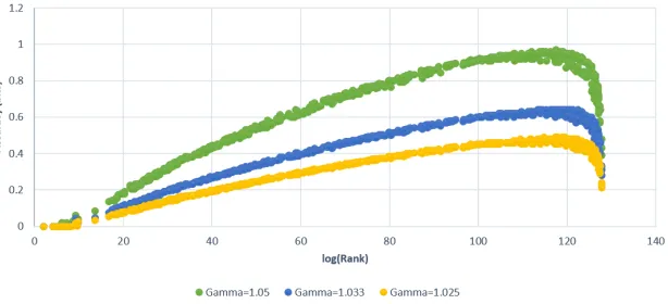
Fig. 2.The accuracy (log2 of the ratio between the upper- and lower-bounds) for the ESrank algorithm as a function of log2(Rank(k∗)) for different parameter settings:
γ= 1.05(green),γ= 1.033(blue),γ= 1.025(yellow).
Sincerank(k∗)might be any value in[low(Rank(k∗), up(Rank(k∗)], we get
accuracy(d, γ) =up(Rank(k∗))/low(Rank(k∗))≤γ2d−2.
E.g., for AES-128 with a preprocessing step of merging the 16 8-bit distributions intod= 8 16-bit distributions we get2d−2 = 14.
Space complexity In the first step we need to store d distributions of size
logγN from Algorithm 4. In order to merge each pair of distributions into one,
we need addition memory of(logγN)2. After merging 2 distributions each of size (logγN), we get one sampled distribution of size(logγN2)which is 2(logγN).
Since we do not need the original pair any more, we can overwrite this space of size2(logγN)and store the new distribution into it. In the same way, in order to merge two distributions of sizelogγN2 we need additional space of (log
γN2)2,
and the merged distribution will overwrite the original pair. In the last step, we need to merge 4 distributions, each of size Nd/4, therefore the maximum additional space we need is(logγNd/4)2. In total we getdlog
γN+ (logγNd/4)2
which is
space(d, γ) =dlogγN+d
2
16(logγN)
2.
4
Empirical Evaluation
Time Space Accuracy < 1 bit
(Seconds) (MB) (%)
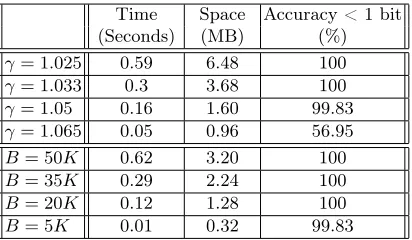
γ= 1.025 0.59 6.48 100 γ= 1.033 0.3 3.68 100 γ= 1.05 0.16 1.60 99.83 γ= 1.065 0.05 0.96 56.95 B= 50K 0.62 3.20 100 B= 35K 0.29 2.24 100 B= 20K 0.12 1.28 100
B= 5K 0.01 0.32 99.83
Table 1. Performance summary of the ESrank and Histogram algorithms. The Ac-curacy column indicates the percentage of traces for which the difference between the upper- and lower-bounds of the estimated ranks was below 1 bit.
For the performance evaluation we used the data of [8]. Within this data corpus there are 611 probability distribution sets gathered from a specific SCA. The SCA of [8] was against AES [1] with 128-bits keys running on an embedded processor with an unstable clock. Each set represents a particular setting of the SCA: number of traces used, whether the clock was jittered, and the values of tunable attack parameters. The attack grouped the key bits into 16 8-bit subkeys, and hence its output probability distributions are over these byte values. Each set in the corpus consists of the correct secret key and 16 distributions, one per subkey. The distributions are sorted in non-increasing order of probability, each of length 28. We used the same technique suggested in [10]: merge the d= 16 probability lists of size N = 28 into d= 8lists of size N = 216. We measured the upper bound, lower bound, time and space for each trace using ESrank and the Histogram rank estimation.
Bound Tightness Figure 2 shows that the analytical performance of section 3.4 indeed agrees with the empirical results. For different values ofγwe get accuracy which corresponds to at mostγ14: e.g., whenγ= 1.05Figure 2 shows a margin of at most0.9bits. We can see that asγbecomes closer to 1, the accuracy becomes closer to 0. As we expected, the maximum gap between the upper bound and the lower bound happens for ranks around100−120since the difference between any two successive indices in the sampled set becomes greater when the indices becomes greater.
run-time of under 1 second using less than 6.5 MB, to get a 1-bit margin of uncertainty in the rank for all ranks up to2128.
5
Conclusion
In this paper we proposed a simple and effective new rank estimation method. We have rigorously analyzed its accuracy, and its time and space complexities. Our main idea is to use exponential sampling to drastically reduce the algo-rithm’s complexity. We proved ESrank has a poly-logarithmic time- and space-complexity, and it can be driven to any desired level of accuracy (trading off time and space against accuracy). Importantly, ESrank is simple to build from scratch, and requires no algorithmic tools beyond a sorting function.
We evaluated the performance of ESrank through extensive simulations based on a real SCA data corpus, and compared it to the currently-best histogram-based algorithm. We showed that ESrank gives excellent rank estimation (with roughly a 1-bit margin between lower and upper bounds), with a performance that is practically on-par with the Histogram algorithm: a run-time of under 1 second, for all ranks up to2128, on a standard laptop. Hence ESrank is a useful addition to the SCA evaluator’s toolbox.
Acknowledgement Liron David was partially supported by The Yitzhak and Chaya Weinstein Research Institute for Signal Processing.
References
1. FIPS PUB 197, advanced encryption standard (AES), 2001. U.S. Department of Commerce/National Institute of Standards and Technology (NIST).
2. D. Agrawal, B. Archambeault, J.R. Rao, and P. Rohatgi. The EM side-channel(s). InCryptographic Hardware and Embedded Systems-CHES 2002, pages 29–45. 2003. 3. Daniel J Bernstein, Tanja Lange, and Christine van Vredendaal. Tighter, faster, simpler side-channel security evaluations beyond computing power. IACR Cryp-tology ePrint Archive, 2015:221, 2015.
4. Andrey Bogdanov, Ilya Kizhvatov, Kamran Manzoor, Elmar Tischhauser, and Marc Witteman. Fast and memory-efficient key recovery in side-channel attacks. InSelected Areas in Cryptography (SAC), 2015.
5. Marios O Choudary and PG Popescu. Back to massey: Impressively fast, scalable and tight security evaluation tools. InInternational Conference on Cryptographic Hardware and Embedded Systems, pages 367–386. Springer, 2017.
6. L. David and A. Wool. A bounded-space near-optimal key enumeration algorithm for multi-subkey side-channel attacks. InProc. RSA Conference Cryptographers’ Track (CT-RSA’17), LNCS 10159, pages 311–327, San Francisco, February 2017. Springer Verlag.
8. D. Fledel and A. Wool. Sliding-window correlation attacks against encryption devices with an unstable clock. In Proc. 25th Conference on Selected Areas in Cryptography (SAC), Calgary, August 2018.
9. Karine Gandolfi, Christophe Mourtel, and Francis Olivier. Electromagnetic anal-ysis: Concrete results. InCryptographic Hardware and Embedded Systems—CHES 2001, pages 251–261. Springer, 2001.
10. Cezary Glowacz, Vincent Grosso, Romain Poussier, Joachim Schueth, and François-Xavier Standaert. Simpler and more efficient rank estimation for side-channel security assessment. InFast Software Encryption, pages 117–129, 2015. 11. Paul Kocher, Joshua Jaffe, and Benjamin Jun. Differential power analysis. In
Advances in Cryptology—CRYPTO’99, pages 388–397. Springer, 1999.
12. Paul C Kocher. Timing attacks on implementations of Diffie-Hellman, RSA, DSS, and other systems. InAdvances in Cryptology—CRYPTO’96, pages 104–113, 1996. 13. Yang Li, Xiaohan Meng, Shuang Wang, and Jian Wang. Weighted key enumera-tion for em-based side-channel attacks. In2018 IEEE International Symposium on Electromagnetic Compatibility and 2018 IEEE Asia-Pacific Symposium on Elec-tromagnetic Compatibility (EMC/APEMC), pages 749–752. IEEE, 2018.
14. Yang Li, Shuang Wang, Zhibin Wang, and Jian Wang. A strict key enumeration algorithm for dependent score lists of side-channel attacks. InInternational Con-ference on Smart Card Research and Advanced Applications, pages 51–69. Springer, 2017.
15. Jake Longo, Daniel P. Martin, Luke Mather, Elisabeth Oswald, Benjamin Sach, and Martijn Stam. How low can you go? using side-channel data to enhance brute-force key recovery. Cryptology ePrint Archive, Report 2016/609, 2016. https: //eprint.iacr.org/2016/609.
16. Daniel P Martin, Luke Mather, and Elisabeth Oswald. Two sides of the same coin: counting and enumerating keys post side-channel attacks revisited. In Cryptogra-phers Track at the RSA Conference, pages 394–412. Springer, 2018.
17. Daniel P Martin, Luke Mather, Elisabeth Oswald, and Martijn Stam. Character-isation and estimation of the key rank distribution in the context of side channel evaluations. InInternational Conference on the Theory and Application of Cryp-tology and Information Security, pages 548–572. Springer, 2016.
18. Daniel P. Martin, Jonathan F. O’Connell, Elisabeth Oswald, and Martijn Stam. Counting keys in parallel after a side channel attack. InAdvances in Cryptology– ASIACRYPT 2015, pages 313–337. Springer, 2015.
19. Jing Pan, Jasper GJ Van Woudenberg, Jerry I Den Hartog, and Marc F Witte-man. Improving dpa by peak distribution analysis. InInternational Workshop on Selected Areas in Cryptography, pages 241–261. Springer, 2010.
20. Romain Poussier, François-Xavier Standaert, and Vincent Grosso. Simple key enumeration (and rank estimation) using histograms: an integrated approach. In
Proc. 18th Cryptographic Hardware and Embedded Systems–CHES 2016, pages 61– 81. Springer, 2016.
21. Jean-Jacques Quisquater and David Samyde. Electromagnetic analysis (EMA): Measures and counter-measures for smart cards. InSmart Card Programming and Security, pages 200–210. Springer, 2001.
23. Nicolas Veyrat-Charvillon, Benoît Gérard, Mathieu Renauld, and François-Xavier Standaert. An optimal key enumeration algorithm and its application to side-channel attacks. InInternational Conference on Selected Areas in Cryptography, pages 390–406. Springer, 2012.
24. Nicolas Veyrat-Charvillon, Benoît Gérard, and François-Xavier Standaert. Security evaluations beyond computing power. In Advances in Cryptology–EUROCRYPT 2013, pages 126–141. Springer, 2013.
25. Shuang Wang, Yang Li, and Jian Wang. A new key rank estimation method to investigate dependent key lists of side channel attacks. In2017 Asian Hardware Oriented Security and Trust Symposium (AsianHOST), pages 19–24. IEEE, 2017. 26. Xin Ye, Thomas Eisenbarth, and William Martin. Bounded, yet sufficient? how to determine whether limited side channel information enables key recovery. In
Smart Card Research and Advanced Applications (CARDIS), pages 215–232. 2014.
Appendix: Proofs
Proof of Lemma 2:
(N∑s−1
i=b+1
ui·(SI[i+ 1]−SI[i]) )
/
(N∑s−1
i=b+1
li·(SI[i]−SI[i−1]) )
≤γ2 (8)
We shall prove that for allb+ 1≤i≤Ns−1
ui·(SI[i+ 1]−SI[i])/li·(SI[i]−SI[i−1])≤γ2
and that will prove Equation (8). From Equation (3) and Equation (4) either li=SI[j−1], ui=SI[j]−1or l1=ui=SI[j], therefore
ui/li ≤γ,
and we only need to prove
(SI[i+ 1]−SI[i])/(SI[i]−SI[i−1])≤γ. (9)
From Lemma 1, it holds that
SI[i+ 1]−SI[i] =⌊(γ−1)·SI[i]⌋
and
SI[i]−SI[i−1] =⌊(γ−1)·SI[i−1]⌋
therefore Equation (9) is
SI[i+ 1]−SI[i]
SI[i]−SI[i−1]=
⌊(γ−1)·SI[i]⌋ ⌊(γ−1)·SI[i−1]⌋ ≤
(γ−1)·SI[i] ⌊(γ−1)·SI[i−1]⌋.
By Lemma 1 Equation (9) is
= (γ−1)· ⌊γ·SI[i−1]⌋ ⌊(γ−1)·SI[i−1]⌋ =
SinceSI[i−1]is an integer it holds
= (γ−1)· ⌊γ·SI[i−1]⌋
⌊γ·SI[i−1]⌋ − ⌊SI[i−1]⌋ =γ−1 +
(γ−1)· ⌊SI[i−1]⌋ ⌊γ·SI[i−1]⌋ − ⌊SI[i−1]⌋
=γ−1 + (γ−1)·SI[i−1]
⌊γ·SI[i−1]−SI[i−1]⌋=γ−1 +
(γ−1)·SI[i−1] ⌊(γ−1)·SI[i−1]⌋≤γ.
⊓ ⊔ Proof of Lemma 3:
((∑b−1
i=1 ui
)
+ub·(SI[b+ 1]−SI[b]) +uNs
)
/
(∑b
i=1 li
)
≤γ2. (10)
We can write this equation in the following way:
( ∑b−1
i=1ui )
+ub·(SI[b+ 1]−SI[b]) +uNs
∑b i=1li
= ∑b
i=1ui ∑b
i=1li
+ub·(SI[b+ 1]−SI[b]−1) +uNs
∑b i=1li
.
Sinceui/li≤γ, Equation (10) is upper bounded by
≤γ+ub·(SI[b+ 1]−SI[b]−1) +uNs
∑b i=1li
.
By Lemma 1 and sincel1≥l2≥...≥lb andub≥uNs, we get
≤γ+ub·((γ−1)·SI[b]−1) +ub
b·lb
.
SinceSI[b] =bandui/li ≤γ
≤γ+γ·lb·(γ−1)·b
b·lb
=γ+γ·(γ−1) =γ2.