Generating finite element method in constructing complex-shaped multigrid finite elements

Generating

finite

element

method

in

constructing complex-shaped multigrid finite

elements

Aleksandr Matveev1,*

1_{ICM SB RAS, 50, bil. 44, Akademgorodok, Krasnoyarsk, Russia, 660036}

Abstract. The calculations of three-dimensional composite bodies based on the finite element method with allowance for their structure and complex shape come down to constructing high-dimension discrete models. The dimension of discrete models can be effectively reduced by means of multigrid finite elements (MgFE). This paper proposes a generating finite element method for constructing two types of three-dimensional complex-shaped composite MgFE, which can be briefly described as follows. An MgFE domain of the first type is obtained by rotating a specified complex-shaped plane generating single-grid finite element (FE) around a specified axis at a given angle, and an MgFE domain of the second type is obtained by the parallel displacement of a generating FE in a specified direction at a given distance. This method allows designing MgFE with one characteristic dimension significantly larger (smaller) than the other two. The MgFE of the first type are applied to calculate composite shells of revolution and complex-shaped rings, and the MgFE of the second type are used to calculate composite cylindrical shells, complex-shaped plates and beams. The proposed MgFE are advantageous because they account for the inhomogeneous structure and complex shape of bodies and generate low-dimension discrete models and solutions with a small error.

1 Introduction

The finite element method (FEM) [1, 2] is widely used to study the stress-strain state (SSS) of complex-shaped elastic composite bodies. In order to simplify calculations, the deformation of bodies of a certain type (for example, beams, plates, shells) is described using engineering theories based on hypotheses [3–9]. However, engineering solutions do not always meet modern requirements. Calculating composite bodies on the basis of the FEM in the formulation of a three-dimensional problem of the elasticity theory [10] with account for their structure can be reduced to constructing high-dimension discrete models, of the order of 1091012. For such discrete models, it is difficult to use computational software such as ANSYS, NASTRAN, etc. [2]. The dimension of discrete models can be effectively reduced by means of the MgFE [11–18], which also serve as a basis for the multigrid finite element method (MFEM) [13–17], based on the FEM

algorithms. The main advantages and features distinguishing the MFEM from the FEM are as follows.

1. In the MFEM (without increasing the dimension of MgFE), one can use arbitrarily small basic partitions of bodies, i.e., MgFE, which allows one to arbitrarily accurately account for their complex shape and inhomogeneous structure, as well as the complex nature of fixing and loading bodies. In the FEM, it is impossible to use arbitrarily small basic partitions because the PC resources are limited, which means that the MFEM is more effective than the FEM.

2. Application the MFEM (based on the basic models of bodies) requires a significantly smaller amount of RAM (103106 times) and time compared to the FEM used for basic models, i.e., the MFEM is more economical than FEM.

3. The MFEM uses homogeneous and composite MgFE constructed using nested grids, which expands the field of application of this method. The FEM uses single-grid homogeneous finite elements (FE). It is noteworthy that boundary-value problems can always be solved using the MFEM instead of the FEM because MgFE can always be used instead of single-grid FE. As mgFE are constructed using m nested grids instead of one (m>1), the MFEM can be regarded as the generalization of the FEM, i.e., the FEM is a special case of the MFEM. Hence, if the FEM-based calculations of bodies are carried out using MgFE, then this case is essentially the implementation of the MFEM.

In this paper, the two types of complex-shaped three-dimensional composite MgFE are designed using the generating FEM. According to this method, the MgFE domain is obtained using the specified displacement of a given complex-shaped plane single-grid FE (below referred to as a generating FE) in a three-dimensional space. The MgFE domain of the first type is obtained by rotating the generating FE around a specified axis at a specified (small) angle, and the MgFE domain of the second type is obtained by the parallel displacement of the generating FE along a specified straight line at a given distance. The nodes of the generating FE are the nodes of a coarse grid of the MgFE, and the nodes of any cross section of the coarse grid of the MgFE are the nodes of the generating FE. This approach simplifies the construction of approximating displacement functions on the coarse grids of the complex-shaped MgFE, where the basis functions of the generating FE are used, and Lagrange polynomials are applied along the direction of the generating FE. The MgFE of the first type are used to calculate the composite shells of revolution, and the MgFE of the second type are used to calculate the composite cylindrical shells of revolution (with a variable curvature radius) and complex-shaped plates and beams. It is assumed that there are ideal bonds between the components of the inhomogeneous structure of the MgFE. The calculation of composite shells of double curvature using the MgFE of the first type is described in [16], and the application of the MgFE of the first and second types for determining the power elements of standard designs is demonstrated in [18].

2 Multigrid FE of the first type. Complex-shaped composite

shells of revolution

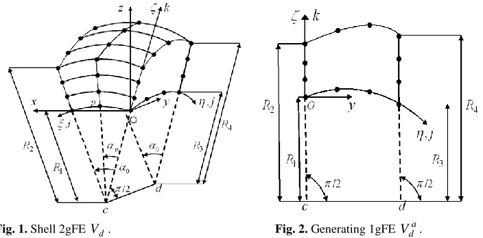
The fundamental principles of constructing the MgFE of the first type, applied to analyze a three-dimensional SSS of composite shells of revolution, are considered on the example of a complex-shaped shell two-grid FE (2gFE), Fig. 1. For the V_d 2gFE, the following local coordinate systems are introduced: Cartesian

Oxyz

, curvilinear O



, and integer

ijk

for the nodes of the coarse grid H_d of the 2gFE. The nodes of the H_d grid for the 2gFE are 36 in number and marked by dots in Fig. 1, with

cd

denoting the shell axis. The generating single-grid FE (1gFE) a

d

V for the V_d 2gFE has 12 nodes of the coarse grid H_d, denoted by dots in Fig. 2. The lateral sides of the a

d

intersection with the

cd

axis. The V_d 2gFE domain is obtained by rotating the generating complex-shaped 1gFE a

d

V around the

cd

axis at the specified angle ₀ (corresponding to partitioning the shell into 2gFE), and



₀ is theapex angle of the V_d 2gFE. The basic partition

d

R of the V_d 2gFE comprises three homogeneous V_e 1gFE of the first order (described in detail in [12]), e1,...,M, and Mis the overall number of the V_e FE. The partition R_d accounts for the inhomogeneous structure and shape of the 2gFE and forms a fine grid h_d, where Hd hd. It is noteworthy that some nodes of the coarse grids of the MgFE can

generally fail to match the nodes of the fine grids. We construct the V_e 1gFE by using the equations of the three-dimensional problem of the elasticity theory [10], written in the local Cartesian coordinate system of the V_e FE[12]. Thus, a three-dimensional SSS is implemented in the 2gFE. Radii R₁ and R3 (R2 and R4) describe the bottom (top) boundaries of the lateral

edges of the 2gFE. In the H_d grid, the displacements functions u_d, v_d, and w_d, used to reduce the dimension of the basic partition R_d, are calculated.

Fig. 1. Shell 2gFE V_d. Fig. 2. Generating 1gFE V_da.

The basis function



_ijk for the i,j,k node of the coarse grid H_d of the V_d 2gFE is

sought in the form

) ( ) , ( ) , , (











_ijk y N_jk y L_i , (1)

where N_jk(y,) denotes the basis functions of the j,k node of the V_da 1gFE,

corresponding to the polynomial P_d(y,) of the form [2]          2 8 2 7 2 6 2 5 4 3 2

1 a y a



a y



a y a



a y



a y



a P_d    3 11 3 10 3

9y a y a y

a





a₁₂



3, j,k1,...,4, L_i() is the second-order Lagrange

polynomial,



     3 , 1 ) ( i p

p i p

p i L    

 , where



_p (_i) is the apex angle of the

p

node

(

i

node), i1,...,3, Fig. 1, and  is the apex angle of the M point lying in the V_d 2gFE domain.

Thus, the basis functions



_ijk of the V_d 2gFE of the first type are represented by power

Denotations N_ 



_ijk, where i1,...,3; j,k1,...,4;



1,...,36. Then, using (1), we

write the displacement functions

u

_d,

v

_d, and

w

_d as



  36 1   u N

ud ,



  36 1   v N

vd ,



  36 1   w N

wd , (2)

where N_, u_, v_, and w_ denote the basis function and displacements of the



-th node of the H_d grid.

The functional of the total potential energy П_d of the base partition

R

_d of the 2gFE is

written in the form

) ] [ 2 1 ( 1 e T e M e e e T e d K

П



δ δ δ P





 , (3)

where [K_e], P_e, and

δ

_e denote the stiffness matrix, nodal force vectors, and

displacement vectors of the V_e1gFE, corresponding to the coordinate system Oxyz of the

d V 2gFE.

Equations (2) are used to express the nodal displacement vector δ_e of the base 1gFE

e

V through the nodal displacement vector δ_d of the coarse grid H_d

(δ_d {u_,v_,w_}T), i.e.

d d e e A δ

δ [ ] , (4)

where [A_ed] denotes the rectangular matrix, e1,...,M .

Equation (4) is substituted into Eq. (3) and the condition П_d(δ_d)/δ_d 0 yields the

relationship [K_d]δ_d F_d, where



  M e d e e T d e

d A K A

K 1 ] ][ [ ] [ ] [ ,



  M e e T d e d A 1 ] [ P

F . (5)

Here [Kd] is the stiffness matrix, and Fdis the nodal force vector of the 2gFE Vd. Let the vector δ_d be determined. Equation (4) is used to calculate vector δ_e of the

nodal displacements of the V_e 1gFE in the coordinate system Oxyz of the V_d 2gFE. The

displacement vector δ*_e of the V_e 1gFE (corresponding to the local Cartesian coordinate

system of the V_e 1gFE) is sought for by the expression δ_e*[M_e]δ_e, where [M_e] is the

rotation matrix [2]. The vector δ*_e and the known algorithms of the FEM [1, 2] are used to

calculate the equivalent stress at the center of the V_e 1gFE domain.

The calculations of the elastic composite round cylindrical shells and panels, carried out using MgFE, are described in [12]. The base functions of the coarse grids of the 2gFE of these shells are determined in the form of Lagrange polynomials and using the power polynomials P(x,y,z) of the first, second, and third orders [12], written in the local

Cartesian coordinate systems. The MgFE of the shells of revolution are verified using the known numerical method [2, 12].

d

V 2gFE domain. Consequently, it is possible to use arbitrarily small basic partitions R_d, allowing one to arbitrarily exactly account for the complex shape and inhomogeneous (microinhomogeneous) structure of the 2gFE V_d and its complex fixing and loading, as

well as to arbitrarily exactly describe a three-dimensional SSS in the V_d 2gFE domain

(with no increase in the dimension of the V_d 2gFE, which is noteworthy).

As shown by the calculations, as the basic partitions of the MgFE become finer, the solution errors decrease. Similarly, the procedures described in Sec. 2 are used to design the composite 2gFE for calculating complex-shaped composite rings and shafts with central circular holes. Three-grid FE (3gFE) of the first type are designed using the 2gFE of the first type with the help of procedures similar to those in Sec. 2

You are free to use colour illustrations for the online version of the proceedings but any print version will be printed in black and white unless special arrangements have been made with the conference organiser. Please check whether or not this is the case. If the print version will be black and white only, you should check your figure captions carefully and remove any reference to colour in the illustration and text. In addition, some colour figures will degrade or suffer loss of information when converted to black and white, and this should be taken into account when preparing them.

3 Multigrid FE of the second type

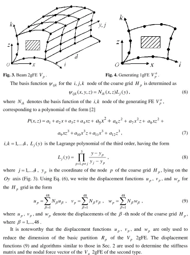
3.1 Multigrid FE for calculating complex-shaped composite beams

The main provisions of the construction procedure for the MgFE of the second type used to analyze the three-dimensional SSS of composite beams are considered on the example of the V_p 2gFE (Fig. 3), which is a complex-shaped rectilinear composite beam with a hole, with the hole section hatched in the figure. The domain of the V_p 2gFE is obtained by the parallel displacement of the generating complex-shaped 1gFE a

p

V (Fig. 4) with a hole

(hatched) along the Oy axis at the specific distance d. The basic partition R_p of the V_p 2gFE consists of the homogeneous 1gFE V_e of the first order, e1,...,M. The partition

p

R accounts for the inhomogeneous structure and complex shape of the V_p 2gFE and forms a fine grid hp, in which the coarse grid Hp of the 2gFE is nested, and the nodes of

the

H

_p grid are marked by points (48 nodes, Fig. 3). The stress state in the V_e 1gFE is described by the equations of the three-dimensional problem of the elasticity theory [10], written in the local Cartesian coordinate system of the V_e FE. Consequently, a three-dimensional SSS is implemented in the V_p 2gFE domain. The nodes of the Vpa 1gFE of

Fig. 3.Beam 2gFE V_p. Fig. 4.Generating 1gFE V_pa.

The basis function



_ijk for the i,j,k node of the coarse grid H_p is determined as

) ( ) , ( ) , ,

(x y z N_ik x z L_j y

ijk 



, (6)

where N_ik denotes the basis function of the i,k node of the generating FE V_pa,

corresponding to a polynomial of the form [2]

   

a a x a z a xz

z x

P( , ) 1 2 3 4



2 5

x

a

2

6z

a a₇x2z a₈xz2

   3 11 3 10 3

9xz a x z a x

a a₁₂z3, (7)

4 ,..., 1 ,k

i , L_j(y) is the Lagrange polynomial of the third order, having the form



     3 , 1 ) ( j p

p j p

p j y y y y y

L , (8)

where j1,...,4, y_p is the coordinate of the node p of the coarse grid H_p, lying on the

Oy axis (Fig. 3). Using Eq. (6), we write the displacement functions u_p, v_p, and w_p for

the H_p grid in the form



  48 1    u N

up ,



  48 1    v N

vp ,



  48 1    w N

wp , (9)

where u_p, v_p, and w_p denote the displacements of the



-th node of the coarse grid H_p,

where  1,...,48.

It is noteworthy that the displacement functions u_p, vp, and wp are only used to

reduce the dimension of the basic partition R_p of the V_p 2gFE. The displacement

functions (9) and algorithms similar to those in Sec. 2 are used to determine the stiffness matrix and the nodal force vector of the V_p 2gFE of the second type.

Note 2. The proposed method allows designing 2gFE whose one characteristic dimension is significantly larger or smaller than all the others. In the Oy directionof the

large dimension of the V_p 2gFE, it is reasonable to use the high order of displacement

approximation (i.e., the high order of the Lagrange polynomials L_j(y)), which allows

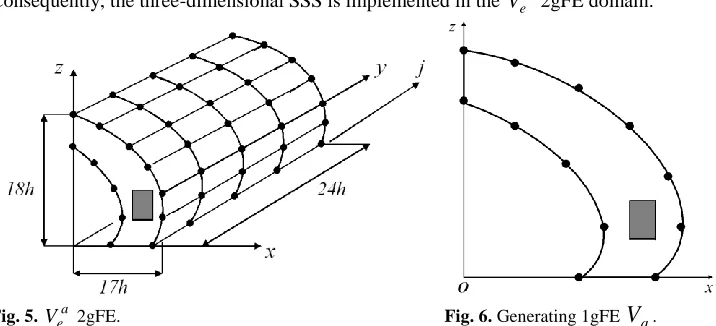
3.2 Multigrid FE for calculating complex-shaped composite cylindrical shells

The construction procedure of the 2gFE of the second type, used to analyze the three-dimensional SSS of cylindrical shells of an inhomogeneous structure and complex shape, is considered on the example of the V_ea 2gFE with characteristic dimensions of

h h

h 24 18

17   (Fig. 5), which has a hole and the section of which is hatched in the figure.

The generatrix (straight line) of the median surface of the V_ea 2gFE is parallel to the Oy

axis (Fig. 5). The V_ea 2gFE domain is obtained by the parallel displacement of the

generating complex-shaped 1gFE V_a (Fig. 6) (the hole section is hatched) along the Oy

axis at a specified distance d24h. The basic partition R_a of the V_ea 2gFE consists of cube-shaped homogeneous 1gFE V_e of the first order with side h, e1,...,M, where

Mdenotes the total number of the V_e FE. The partition R_a accounts for the

inhomogeneous structure and complex shape of the V_ea 2gFE and forms a fine grid h_a, in

which the coarse grid H_a of the 2gFE is nested (H_a h_a). The nodes of the coarse grid

a

H are marked in Fig. 5 by points (60 nodes). The nodes of the V_a 1gFE of the third order are the nodes of the coarse grid H_a, marked by points (12 nodes, Fig. 6). A stress state in

the V_e 1gFE is described by the equations of the three-dimensional problem of the

elasticity theory [10] (written in the local Cartesian coordinate system of the V_e FE).

Consequently, the three-dimensional SSS is implemented in the V_ea 2gFE domain.

Fig. 5.V_ea 2gFE. Fig. 6. Generating 1gFE

V

_a.

For the pair of numbers i,j, where i1,...,12, j1,...,5, we determine an integer

1





,



1,...,60. The basis function _(x,y,z) for the



-th node in the coarse grid of the V_ea 2gFE is sought in the form

) ( ) , ( ) , ,

(x y z N_i x z L_j y 



, (10)

where  1,60, Ni(x,z) is the shape function of the

i

th node of the generating 1gFE Va,

12 ,..., 1 

i , corresponding to the polynomial P(x,z), presented in the local Cartesian coordinate system Oxz (Fig. 6), of the form (7), L_j(y) is the fourth-order Lagrange

polynomial (Eq. (8)), where j1,...,5, y_p is the coordinate of the p node of the coarse

In Eq. (10), the basis functions _ 2gFE V_ea of the second type are represented by power polynomials, i.e., functions of the form Ni(x,z) of the generating FE Va, and by

the Lagrange polynomials L_j(y) in the direction of the generating FE (along the Oyaxis).

Using Eq. (10), we write the displacement functions u_a, v_a, and w_a for the coarse grid

a H as





 60

1

   u N

ua ,





 60

1

   v N

va ,





 60

1

   w N

wa , (11)

where N_, u_, v_, and w_ denote the basis function and displacements of the



-th node of the H_a grid.

It is noteworthy that the displacement functions u_a, v_a, and w_a are only used to

reduce the dimension of the basic partition R_a of the 2gFE V_ea. We use the displacement functions (11) and the algorithms similar to those in Sec. 2 to determine the stiffness matrix

and the nodal force vector of the V_ea 2gFE of the second type.

3.3 Multigrid FE for calculating complex-shaped composite plates

We consider the construction procedure for the 2gFE of the second type in order to analyze the three-dimensional SSS of plates with an inhomogeneous structure on the example of the

complex-shaped composite laminated 2gFE V_gb (Fig. 7), where Oxyzis the Cartesian

coordinate system. The characteristic dimensions B and Hof the Vgb 2gFE significantly

exceed the dimension of h, with h being the thickness of the 2gFE. The V_gb 2gFE domain

is obtained by the parallel displacement of the generating 1gFE V_g (Fig. 8) along the Oy

axis at the given distance h. The coarse grid of the V_gb 2gFE has 27 nodes marked by

points in Fig. 7. The basic partition of the Vgb 2gFE consists of cube-shaped homogeneous

FE of the first order (rectangular parallelepiped [2]), in which a three-dimensional SSS is implemented. It is noteworthy that the basic partitions of the 2gFE can be arbitrarily small, i.e., can arbitrarily exactly account for the inhomogeneous structure and complex shape of

the 2gFE. The base function _(x,y,z) for the



-th node in the coarse grid of the V_gb 2gFE is sought in the form (6), where



1,...,27, Ni(x,z) is the shape function of the

i-th node of the generating 1gFE V_g, i1,...,9, corresponding to a polynomial of the

form 9 2 2

2 8 2 7 2 6 2 5 4 3 2 1

) ,

(x z a a x a z a xz a x a z a x z a xz a x z

P_g          , presented

in the local Cartesian coordinate system Oxz, Fig. 8, and L_j(y) denotes the Lagrange

Fig. 7. Laminated 2gFE Vgb. Fig. 8. Generating 1gFE Vg.

The stiffness matrix and nodal force vector of the laminated 2gFE V_gb are determined

using procedures similar to those in Secs. 3.1 and 3.2. The discrete models of the plates are

generally comprised of complex-shaped 2gFE (such as curvilinear 2gFE Vgb) and 2gFE

shaped as a rectangular parallelepiped, constructed with the help of power polynomials [2], and Lagrange polynomials [12]. It is noteworthy that the proposed MgFE of the first and second types can be used in analyzing the three-dimensional SSS of corrugated plates, panels, and floors [19, 20] (corrugation can be shaped as a trapezium, rectangle, triangle, a part of a circular arc, etc.). Three-grid FE (3gFE) of the second type are designed using the 2gFE of the second type with the help of procedures similar to those in Secs. 2, 3.2, and 3.3.

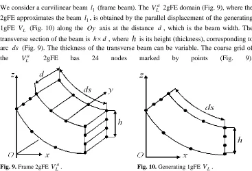
3.4 Multigrid FE for calculating curvilinear composite beams

We consider a curvilinear beam l₁ (frame beam). The V_La 2gFE domain (Fig. 9), where the

2gFE approximates the beam l₁, is obtained by the parallel displacement of the generating

1gFE V_L (Fig. 10) along the Oy axis at the distance d, which is the beam width. The

transverse section of the beam is hd , where

h

is its height (thickness), corresponding to arc ds (Fig. 9). The thickness of the transverse beam can be variable. The coarse grid of the V_La 2gFE has 24 nodes marked by points (Fig. 9).

The basis function _(x,y,z) for the



-th node of the coarse grid of the V_La 2gFE is determined in the form (10), where



1,...,24, Ni(x,z) denotes the shape function of the

i-th node of the generating 1gFE V_L (Fig. 10), i1,...,12, corresponding to a polynomial of the form (7), written in the local Cartesian coordinate system Oxz (Fig. 10), and L_j(y)

denotes the Lagrange polynomials of the first order. i1,...,12. The stiffness matrix and

nodal force vector of the V_La 2gFE are determined in procedures similar to those in Secs. 3.2 and 3.3.

4 Conclusion

In this paper, three-dimensional composite and homogeneous MgFE of two types of complex shapes are considered, which are designed with the use of forming FE. The procedures for the construction of type 1 and type 2 MgFE are described, which are used for the calculation of composite (homogeneous) shells of rotation, cylindrical shells (with a variable radius of curvature), plates and beams of complex shape. The main advantages of the proposed MgFE are that they take into account the inhomogeneous, micro-inhomogeneous structure and complex shape of bodies, describe three-dimensional behavior in composite (homogeneous) bodies, form discrete models of small dimension and generate approximate solutions with a small error.

References

1. O.C. Zienkiewicz. The Finite Element Method in Engineering Science (McGraw-Hill, London, 1971)

2. D.H. Norrie and G. de Vries. An Introduction to Finite Element Analysis (Academic Press, New York, San Francisco, London, 1978)

3. A.P. Kiselev, N.A. Gureeva, R.Z. Kiselyova, Izv. Vuzov. Stroitel’stvo, 1, 106-112 (2010)

4. S.K. Golushko, Yu.V. Nemirovskii. Direct and Inverse Problems of the Mechanics of Elastic Composite Plates and Shells of Revolution (Fizmatlit, Moscow, 2008)

5. A. Ahmed A, S. Kapuria, Composite Structures, 158, 112–127 (2016)

6. E. Carrera, A. Pagani, S. Valvano, Composites Part B: Engineering, 111, 294 –314 (2017)

7. M.Y. Yasin, S. Kapuria, Composite Structures, 98, 202–214 (2013) 8. M. Cinefra, E. Carrera, Int. J. Num. Meth. Eng. 93, 2, 160-182 (2013)

9. M.F. Сaliri, A. J.M. Ferreira, V. Tita, Composite Structures, 156, 63–77 (2016)

10. V.I. Samul’. Fundamentals of the Theory of Elasticity and Plasticity (Vysshaya Shkola, Moscow, 1982)

11. A.D. Matveev, Vestnik Krasnoyarskogo Gosudarstvennogo Agrarnogo Universiteta, 3, 44-47 (2014)

13. A. D. Matveev. The Multigrid Finite Element Method in Calculating Three-Dimensional Homogeneous and Composite Solids. Uchen. Zap. Kazan. Univ. Ser.: Fiz.-Matem. Nauki, 158, No. 4, 530-543 (2016)

14. A.D. Matveev, Vestnik KrasGAU, 11, 131-140 (2017) 15. A.D. Matveev, Vestnik KrasGAU, 2, 90-103 (2018)

16. A.D. Matveev, Vestnik KrasGAU, 3, 126-137 (2018)

17. A.D. Matveev, IOP Conf. Ser.: Mater. Sci. Eng. 158, 1, 012067, 1-9 (2016)

18. A.D. Matveev, Vestnik KrasGAU, 6, 141-154 (2018)

19. Y Xia, M.I. Friswell, E.I Saavedra Flores, Itern. J. Solids Structures 49, 14, 1453-1462 (2012)