A Note on
‘Further Improving Efficiency of
Higher-Order Masking Schemes by
Decreasing Randomness Complexity’
“Almost” is Like “Not At All”
Gilles Barthe
1, Fran¸cois Dupressoir
2, and Benjamin Gr´
egoire
31
IMDEA Software Institute
2
University of Surrey ([email protected])
3
Inria M´
editerran´
ee
Abstract. Zhang, Qiu and Zhou [5] propose two optimised masked algo-rithms for computing functions of the formx7→x·`(x) for any linear function
`. They claim security properties. We disprove their first claim by exhibiting a first order flaw that is present in their first proposed algorithm scheme at all orders. We put their second claim into question by showing that their proposed algorithm, as published, is not well-defined at all orders, making use of variables before defining them. We then also exhibit a counterexample at order 2, that we believe generalises to all even orders.
Coron, Prouff, Rivain and Roche [3] (CPRR) introduced specialised masked algorithms for computing a particular functionality of interest that had so far been problematic from the point of view of security: functions of the formx7→x·`(x) for some lineary function`. Their proposed algorithm–if it improves time complexity–does not, however, improve on the randomness complexity of the simpler option of simply composing a gadget for`and a multiplication gadget, taking care to insert the necessary mask refreshing operation.
Zhang, Qiu and Zhou [5] (ZQZ) recently proposed two masked algorithms for com-puting these functionalities that have reduced randomness complexity. They claim that their algorithms enjoy particularprobing security properties. In this short note, we give counterexamples to these claims.
1. Definitions
We limit our definitions to the relevant case here: that of gadgets with a single input and a single output.
Definition 1(t-Non-Interference). A gadget is t-Non-Interfering(ort-NI) whenever the joint distribution of any d ≤ t of its intermediate variables can be perfectly simulated using at mostt shares of its input.
Definition 2 (t-Strong-Non-Interference). A gadget is t-Strongly-Non-Interfering (or
t-SNI) whenever the joint distribution of any t1 of its intermediate variables and t2 of
its output shares (with t1+t2 ≤t) can be perfectly simulated using at most t1 shares of
its input.
We use the “simulation” terminology of Ishai, Sahai and Wagner [4] and others, but note that the simulations here are not meant in the usual cryptographic sense. When we write that a distribution d(a0, . . . , at) (expressed as a function of the input shares
a0, . . . , at since it is the joint distribution of adversary probes) can besimulated using
at most n < t shares of a gadget’s input, we mean that there exists an n-ary function
d0 such that for alla0, . . . , at, we have d0(aπ1, . . . , aπn) =d(a0, . . . , at). (In other words,
the distribution is fully determined by the value of at most n shares of the input.) We note in particular that this property makes no assumption on the distribution of inputs, but rather keeps both the real and simulated distribution dependent on it.
With this in mind, in order to break claims of NI or SNI security, it is sufficient to exhibit a set of intermediate variables whose distribution clearly depends on more than the allowed number of input shares. This is the approach we take here.
2. First Proposal
Algorithm 1 shows the first ZQZ proposal, which they claim is t-SNI for allt (and any linear function `). The algorithm, as the original proposal by Coron et al. [3], assumes leak-free lookups in a tableh such thath[x] =x·`(x) for any x.
2.1. A First-Order Flaw
We now exhibit a first-order flaw in this algorithm that is present at any order, and in any (boolean) ring or field. In order to show that Algorithm 1 is not 1-SNI, it is sufficient to exhibit either:
1. An intermediate variable whose distribution cannot be perfectly simulated (or predicted) given only one share of the input; or
2. An output variable whose distribution cannot be perfectly simulated (or predicted) without any knowledge about the input shares.
Algorithm 1 The First ZQZ Proposal [5] (Algorithm 2)
function Ht1(a, h)
fori= 0 tot do
for j=i+ 1totdo
ri,j ←$ F2n ti,j
$
←h[ri,j] +h[ai+ri,j]
tj,i
$
←h[ai+ri,j+aj] +h[aj +ri,j]
fori= 0 tot do ci←h[ai]
for j= 0 tot,j6=i do ci ←ci+ti,j
return c
ZQZ.1
The final value of c0 at order tcan be expressed as follows:
c0 =a0·`(a0) +
t
X
j=1
r0,j·`(r0,j) + (a0+r0,j)·`(a0+r0,j)
We now show that the distribution of this expression cannot be predicted without knowledge of a0. First observe that, for a0 = 0, the distribution of c0 is the point
distribution that gives probability 1 to element 0. Indeed, note that:
c0 =a0·`(a0) +Ptj=1r0,j·`(r0,j) + (a0+r0,j)·`(a0+r0,j)
= 0 +Pt
j=1r0,j·`(r0,j) + r0,j·`(r0,j)
= 0
It is also easy to see that, if the same (constantly 0) distribution is obtained for other values of a0, then an adversary can obtain the value of c = a·`(a) by observing the
remainingt shares of c(c1, . . . , ct) and recombining them.
Therefore, it is the case that either i. the distribution of c0 depends on a0 (and in
particular, an adversary observing a value ofc0 6= 0 could infer thata0 6= 0); or ii. there
is a set oft observations that reveals the value ofa.
Either of these situations is a counterexample to ZQZ’s security claim. We exhibit a detailed breakdown of the flaw witht= 1,n= 2 and instantiating`as the function that swaps the bits of its arguments, in Appendix A.
3. Second proposal
Algorithm 2 shows what we understand is the second ZQZ proposal [5], which they claim ist-NIfor all t(and all `).
1
We first note that the Algorithm is not well-defined for odd values of t. Indeed, in such cases, the loop at Line 5 initialises only those rj for even values of j such that
0< j < t. However, Line 17 makes use of ri for all odd values of isuch that 0 < i≤t
(regardless of the order). In the following, we do not pretend to fix this proposal, and only consider the security of Algorithm 2 for even values oft.2
Algorithm 2 The Second ZQZ Proposal [5] (Algorithm 3)
1: function Ht2(a, h)
2: for i= 0 totdo
3: forj= 0 to t−i−1 by2 do
4: ri,t−j ←$ F2n
5: for j=t−1 downto1by 2 do
6: rj
$
←F2n
7: for i= 0 totdo
8: ci ←h[ai]
9: forj=tdowntoi+ 2by 2 do
10: ti,j ←h[ai+ri,j] +h[ri,j] +h[ai+rj−1] +h[rj−1]
11: ci←ci+ti,j
12: if i mod 26=t mod 2 then
13: ti,i+1 ←h[ai+ri,i+1] +h[ri,i+1]
14: ci←ci+ti,i+1
15: if i mod 2 = 1then
16: for j=i−1 downto0do
17: ti,j ←h[ai+ri+aj] +h[ai+ri] 18: ci ←ci+ti,j
19: else
20: for j=i−1 downto0do
21: ti,j ←h[rj,i] +h[ai+rj,i] 22: ci ←ci+ti,j
23: return c
3.1. Counterexample
We instantiate Algorithm 2 witht= 2 (as Algorithm 3).
Consider the final distribution ofc1and note that, since`is linear and the distribution
ofr1(resp. r1,2) is the same as that ofa1+r1(resp. a1+r1,2, we have, denoting “equality
of distributions knowing thatr is distributed uniformly” using∼=r:
2
It is likely that the loop at Line 5 can be fixed to always initialise rj with j odd. The presence of
Algorithm 3 Algorithm 2 witht= 1
function H22(a, h)
r0,2 $
←F2n r1,2 ←$ F2n r1 ←$ F2n c0 ←h[a0]
t0,2←h[a0+r0,2] +h[r0,2] +h[a0+r1] +h[r1]
c0 ←c0+t0,2
c1 ←h[a1]
t1,2←h[a1+r1,2] +h[r1,2]
c1 ←c1+t1,2
t1,0←h[a1+r1+a0] +h[a1+r1]
c1 ←c1+t1,0
c2 ←h[a2]
t2,1←h[r1,2] +h[a2+r1,2]
c2 ←c2+t2,1
t2,0←h[r0,2] +h[a2+r0,2]
c2 ←c2+t2,0
return hc0,c1,c2i
c1 = a1·`(a1) + (a1+r1,2)·`(a1+r1,2) +r0,2·`(r0,2)
+(a1+r1+a0)·`(a1+r1+a0) + (a1+r1)·`(a1+r1)
∼
=r1,2 a1·`(a1) +r1,2·`(r1,2) +r0,2·`(r0,2)
+(a1+r1+a0)·`(a1+r1+a0) + (a1+r1)·`(a1+r1)
∼
=r1 a1·`(a1) +r1,2·`(r1,2) +r0,2·`(r0,2) + (r1+a0)·`(r1+a0) +r1·`(r1)
= a0·`(a0) +a1·`(a1) +r1·`(a0) +a0·`(r1) +r1,2·`(r1,2) +r0,2·`(r0,2)
Tables 1 and 2 detail the distribution of c1 as a function of a0 and a1 with t = 2,
n = 2, and `= x 7→ x1. When distributions are single-valued, we simply give that value. In other cases we describe the probability mass function, omitting elements of probability 0. Detailed computations for the distribution of r1·(a01) +a0·(r11)
are given in Table 3, in an Appendix which also includes a table for the computation of
·inF22 (Table 4). We also note that, for anyx, we have
x·(x1) =
00 ifx= 00
10 otherwise.
As a consequence, the distribution of r1,2·`(r1,2) +r0,2·`(r0,2), independent of a0 and
a1 is simply expressed as
007→ 5 8; 107→
3 8 .
The flaw here is more subtle: we need to show that predicting the distribution of c1
requires information on both a0 and a1.
When a0 = 00, the distribution of c1 clearly depends on a1 (as shown in the first
a0 a1 a0·(a01) a1·(a11) r1·(a01) +a0·(r11) c1
00 00 00 00 00
007→ 5 8; 107→
3 8
00 01 00 10 00
007→ 3 8; 107→
5 8
00 10 00 10 00
007→ 3 8; 107→
5 8
00 11 00 10 00
007→ 3 8; 107→
5 8
01 00 10 00
007→1 2; 107→
1 2
007→ 1 2; 107→
1 2
01 01 10 10
007→1 2; 107→
1 2
007→ 1 2; 107→
1 2
01 10 10 10 007→1
2; 107→ 1 2
007→ 1 2; 107→
1 2
01 11 10 10
007→1 2; 107→
1 2
007→ 1 2; 107→
1 2
10 00 10 00
007→1 2; 107→
1 2
007→ 1 2; 107→
1 2
10 01 10 10
007→1 2; 107→
1 2
007→ 1 2; 107→
1 2
10 10 10 10
007→1 2; 107→
1 2
007→ 1 2; 107→
1 2
10 11 10 10
007→1 2; 107→
1 2
007→ 1 2; 107→
1 2
11 00 10 00
007→1 2; 107→
1 2
007→ 1 2; 107→
1 2
11 01 10 10
007→1 2; 107→
1 2
007→ 1 2; 107→
1 2
11 10 10 10
007→1 2; 107→
1 2
007→ 1 2; 107→
1 2
11 11 10 10
007→1 2; 107→
1 2
007→ 1 2; 107→
1 2
Table 1: Distribution of c1 as a function ofa0.
a1 a0 a1·(a11) a0·(a01) r1·(a01) +a0·(r11) c1
00 00 00 00 00
007→ 5 8; 107→
3 8
00 01 00 10
007→1 2; 107→
1 2
007→ 1 2; 107→
1 2
00 10 00 10
007→1 2; 107→
1 2
007→ 1 2; 107→
1 2
00 11 00 10
007→1 2; 107→
1 2
007→ 1 2; 107→
1 2
01 00 10 00 00
007→ 3 8; 107→
5 8
01 01 10 10
007→1 2; 107→
1 2
007→ 1 2; 107→
1 2
01 10 10 10
007→1 2; 107→
1 2
007→ 1 2; 107→
1 2
01 11 10 10
007→1 2; 107→
1 2
007→ 1 2; 107→
1 2
10 00 10 00 00
007→ 3 8; 107→
5 8
10 01 10 10 007→1
2; 107→ 1 2
007→ 1 2; 107→
1 2
10 10 10 10
007→1 2; 107→
1 2
007→ 1 2; 107→
1 2
10 11 10 10
007→1 2; 107→
1 2
007→ 1 2; 107→
1 2
11 00 10 00 00
007→ 3 8; 107→
5 8
11 01 10 10
007→1 2; 107→
1 2
007→ 1 2; 107→
1 2
11 10 10 10
007→1 2; 107→
1 2
007→ 1 2; 107→
1 2
11 11 10 10
007→1 2; 107→
1 2
007→ 1 2; 107→
1 2
Similarly, whatever the value ofa1, the distribution ofc1 varies with the value ofa0.
This is shown more clearly in Table 2.
The leak exhibited here is clearly more subtle than that on the first proposal, for several reasons:
1. although we suspect similar flaws exist at higher orders, in other structures and for other instantiations for`, we only explicitly exhibit it fort= 2 and in the case wheren= 2 and` is the 1-bit rotation function;
2. rather than a single observation leaking information about the input, the flaw on the second proposal requires the adversary to estimate the distribution of c1 (by
performing multiple measurements) to infer the information.
The bias we exhibit is quite small, but exists, and therefore contradicts the claims of perfect probing security made by the original authors.
4. Analysis, Discussion and Conclusions
In this short note, we have exhibited counterexamples to both of Zhang, Qiu and Zhou’s core theorems [5]. However, their compositional proof for the AES SBox would remain valid given at-NIgadget with reduced randomness complexity that computesx7→x·`(x), and searching for such a gadget remains a valuable research objective.
We do not claim that the leakage we exhibit here could be exploited in practice, but simply wish to bring attention to the fact that the gadgets proposed by Zhang, Qiu and Zhou are not as secure as claimed, and may therefore not be suitable for practical security-critical applications, despite their improved randomness complexity.
The counterexamples shown here were found using Barthe et al.’smaskVerif tools [1, 2]. Since the proof techniques used in those tools are incomplete (that is, they may fail to prove true statements), the counterexamples were further verified and refined by hand (and the first flaw generalised). This short note and its use of formal verification tools further illustrate, if it was still needed, the value of formal methods and automated verification tools in the domain of provably secure masked algorithms, for which proofs are notoriously tedious, error prone and difficult to check.
References
[1] Gilles Barthe, Sonia Bela¨ıd, Fran¸cois Dupressoir, Pierre-Alain Fouque, Benjamin Gr´egoire, and Pierre-Yves Strub. Verified proofs of higher-order masking. In
Elisa-beth Oswald and Marc Fischlin, editors, EUROCRYPT 2015, Part I, volume 9056
of LNCS, pages 457–485. Springer, Heidelberg, April 2015.
[2] Gilles Barthe, Sonia Bela¨ıd, Fran¸cois Dupressoir, Pierre-Alain Fouque, Benjamin Gr´egoire, Pierre-Yves Strub, and R´ebecca Zucchini. Strong non-interference and
type-directed higher-order masking. In Edgar R. Weippl, Stefan Katzenbeisser,
Christopher Kruegel, Andrew C. Myers, and Shai Halevi, editors, ACM CCS 16,
[3] Jean-S´ebastien Coron, Emmanuel Prouff, Matthieu Rivain, and Thomas Roche. Higher-order side channel security and mask refreshing. In Shiho Moriai, editor,
FSE 2013, volume 8424 ofLNCS, pages 410–424. Springer, Heidelberg, March 2014.
[4] Yuval Ishai, Amit Sahai, and David Wagner. Private circuits: Securing hardware
against probing attacks. In Dan Boneh, editor, CRYPTO 2003, volume 2729 of
LNCS, pages 463–481. Springer, Heidelberg, August 2003.
[5] Rui Zhang, Shuang Qiu, and Yongbin Zhou. Further improving efficiency of higher
order masking schemes by decreasing randomness complexity. IEEE Transactions
on Information Forensics and Security, 12(11), November 2017.
A. A Detailed Look at the First Proposal
We now give a detailed account of a particular instance of the flaw we exhibit on ZQZ’s first proposal (Algorithm 1. We instantiate Algorithm 1 fort= 1 (as Algorithm 4) and exhibit a single output share whose distribution varies witha0, and therefore cannot be
simulated without knowledge about that input share. This violates the 1-SNI property claimed by ZQZ [5].
Algorithm 4 Algorithm 1 witht= 1
function H11(a= (a0,a1), h)
r0,1 ←$ F2n
t0,1←h[r0,1] +h[a0+r0,1]
t1,0←h[a0+r0,1+a1] +h[a1+r0,1]
c0 ←h[a0]
c0 ←c0+t0,1
c1 ←h[a1]
c1 ←c1+t1,0
return hc0,c1i
Consider the distribution of the final value of c0, and note that, since ` is linear, we
have:
c0 = a0·`(a0) +r0,1·`(r0,1) + (a0+r0,1)·`(a0+r0,1)
= a0·`(a0) +r0,1·`(r0,1) +a0·`(a0) +a0·`(r0,1) +r0,1·`(a0) +r0,1·`(r0,1)
= a0·`(r0,1) +r0,1·`(a0)
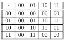
For example, choosing n= 2 and`(x) =x1 (the left rotation on binary words), it is clear that the distribution ofc0 does in fact depend on the value ofa0. For example, if
a0 = 00, thenc0= 00 for all possible values of r0,1, whereas other values ofa0 yield the
same two-valued distribution onc0 (see Table 3; Table 4 recalls multiplication in F22).
a0 r0,1 a01 r0,11 a0·(r0,11) r0,1·(a01) r0,1·(a01) +a0·(r0,11)
00 00 00 00 00 00 00
00 01 00 10 00 00 00
00 10 00 01 00 00 00
00 11 00 11 00 00 00
01 00 10 00 00 00 00
01 01 10 10 10 10 00
01 10 10 01 01 11 10
01 11 10 11 11 01 10
10 00 01 00 00 00 00
10 01 01 10 11 01 10
10 10 01 01 10 10 00
10 11 01 11 01 11 10
11 00 11 00 00 00 00
11 01 11 10 01 11 10
11 10 11 01 11 01 10
11 11 11 11 10 10 00
Table 3: Distribution of c0 as a function ofa0: detailed computation.
· 00 01 10 11
00 00 00 00 00
01 00 01 10 11
10 00 10 11 01
11 00 11 01 10