Quantum algorithms for computing general discrete
logarithms and orders with tradeoffs
Martin Eker˚
a
1,2 1KTH Royal Institute of Technology, Stockholm, Sweden
2
Swedish NCSA, Swedish Armed Forces, Stockholm, Sweden
March 30, 2020
Abstract
We generalize our earlier works on computing short discrete logarithms with tradeoffs, and bridge them with Seifert’s work on computing orders with tradeoffs, and with Shor’s groundbreaking works on computing orders and general discrete logarithms. In particular, we enable tradeoffs when com-puting general discrete logarithms.
Compared to Shor’s algorithm, this yields a reduction by up to a factor of two in the number of group operations evaluated quantumly in each run, at the expense of having to perform multiple runs. Unlike Shor’s algorithm, our algorithm does not require the group order to be known. It simultaneously computes both the order and the logarithm.
We analyze the probability distributions induced by our algorithm, and by Shor’s and Seifert’s order finding algorithms, describe how these algorithms may be simulated when the solution is known, and estimate the number of runs required for a given minimum success probability when making different tradeoffs.
1
Introduction
As in [3, 4, 5], letGunderbe a finite cyclic group of orderrgenerated byg, and
x= [d]g=gg · · · g
| {z }
dtimes
.
The discrete logarithm problem is to computed= loggxgiven the group elements
g andx. In cryptographic applications, the groupGis typically a subgroup of F∗p, for some primep, or an elliptic curve group.
In the general discrete logarithm problem 0≤d < r, whereasdis smaller thanr
by some order of magnitude in the short discrete logarithm problem.
1.1
Earlier works
compute discrete logarithms in arbitrary finite cyclic groups, provided the group operation can be implemented efficiently on the quantum computer.
Eker˚a [3] initiated a line of research in 2016 by introducing a modified version of Shor’s algorithm for computing discrete logarithms that more efficiently solves the short discrete logarithm problem. This work is of cryptographic significance as the short discrete logarithm problem underpins many implementations of cryptographic schemes instantiated with safe-prime groups. A notable example is Diffie-Hellman key exchange [2] in TLS, IKE and NIST SP 800-56A [23, 22, 21].
In a follow-up work, Eker˚a and H˚astad [4] enabled tradeoffs in Eker˚a’s algo-rithm using ideas that directly parallel those of Seifert [18] in his work on enabling tradeoffs in Shor’s order finding algorithm; the quantum part of Shor’s factoring algorithm. Eker˚a and H˚astad furthermore showed how the RSA integer factoring problem, that underpins the widely deployed RSA cryptosystem [16], may be re-duced via [7] to a short discrete logarithm problem and attacked quantumly. This gives rise to a quantum algorithm that more efficiently solves the RSA integer factoring problem than Shor’s original factoring algorithm when making tradeoffs. Eker˚a [5] subsequently refined the classical post-processing in [4] to render it more efficient. With this improved post-processing, the algorithm of Eker˚a and H˚astad was shown in [5] to outperform Shor’s factoring algorithm when targeting RSA integers, irrespective of whether tradeoffs are made.
A key component to this result was the development of a classical simulator for the quantum algorithm for computing short discrete logarithms: For problem instances for which the solution is classically known, this simulator allows outputs to be generated that are representative of outputs that would be generated by the quantum algorithm if executed on a quantum computer. This in turn allows the efficiency of the classical post-processing to be experimentally assessed.
1.2
Our contributions
We generalize and bridge our earlier works on computing short discrete logarithms with tradeoffs, Seifert’s work on computing orders with tradeoffs and Shor’s ground-breaking works on computing orders and general discrete logarithms. In particular, we enable tradeoffs when computing general discrete logarithms.
Compared to Shor’s algorithm for computing general discrete logarithms, this yields a reduction by up to a factor of two in the number of group operations evaluated quantumly in each run, at the expense of having to perform multiple runs. Unlike Shor’s algorithm, our algorithm does not require the group order to be known. It simultaneously computes both the order and the logarithm. This allows it to outperform Shor’s original algorithms with respect to the number of group operations that need to be evaluated quantumly in some cases even when not making tradeoffs. One cryptographically relevant example of such a case is the computation of discrete logarithms in Schnorr groups of unknown order.
We analyze the probability distributions induced by our algorithm, and by Shor’s and Seifert’s order finding algorithms, describe how all of these algorithms may be simulated when the solution is known, and estimate the number of runs required for a given minimum success probability when making different tradeoffs.
1.2.1 On the cryptographic significance of this work
In this work, we further the understanding of how hard these two key problems are to solve quantumly when not on special form. We hope that our results may prove useful when developing cost estimates for quantum attacks, and that they may inform decisions on when to mandate migration from the currently deployed asymmetric cryptosystems to post-quantum secure cryptosystems.
1.2.2 Further details and overview
Our algorithm for computing discrete logarithms consists of two algorithms;
• a quantum algorithm, that upon input of a generatorg of order r, and an elementx= [d]gwhere 0≤d < r, outputs a pair (j, k), and
• a classical probabilistic post-processing algorithm, that upon input of a set ofnpairs (j, k), produced bynruns of the quantum algorithm, computesd.
In addition to the above post-processing algorithm, we furthermore specify
• a classical probabilistic post-processing algorithm, that upon input of a set ofnpairs (j, k), computes the orderr. Note that the same set of pairs may be used as input to both this and the above post-processing algorithm.
The quantum algorithm is identical to the algorithm in [4, 5] for computing short discrete logarithms with tradeoffs. The key difference in this work is that we admit general discrete logarithms and comprehensively analyze the probability distribution that the algorithm induces for such logarithms. The post-processing algorithm for dis a tweaked version of the lattice-based algorithm in [5], whereas the algorithm forris a natural generalization of the lattice-based algorithm in [5] first sketched in a pre-print of [4]. It is similar to the post-processing in [18].
The quantum algorithm is parameterized under a tradeoff factors. This factor controls the tradeoff between the requirements that the algorithm imposes on the quantum computer, and the number of runs,n, required to attain a given minimum probability qof recoveringdandrin the classical post-processing.
Following [5], we estimate n for a given problem instance, represented by d
and r, and fixed s and q, by simulating the quantum algorithm. We first use the simulated output to heuristically estimate n, and then verify the estimate by executing the two post-processing algorithms with respect to simulated output.
The simulator is based on a high-resolution two-dimensional histogram of the probability distribution induced by the quantum algorithm. By sampling the histo-gram, we generate pairs (j, k) that very closely approximate the output that would be produced by the quantum algorithm if executed on a quantum computer.
To construct the histogram, we first derive a closed form expression that approx-imates the probability of the quantum algorithm yielding (j, k) as output, and an upper bound on the error in the approximation. We then integrate this expression and the error bound numerically in different regions of the plane.
Our simulations show that when not making tradeoffs, a single run suffices to computed or r with≥99% success probability. When making tradeoffs, slightly more thansruns are typically required to achieve a similar success probability. In appendix A we show that these results extend to order finding and factoring.
1.2.3 Structure of this paper
The quantum algorithm is described in section 2. In section 3, we analyze the probability distribution it induces, and derive a closed form expression that ap-proximates the probability of it yielding (j, k) as output. In sections 4 and 5, we describe how the high-resolution histogram is constructed by integrating the closed form expression, and how it is sampled to simulate the quantum algorithm.
In section 6, we describe the two post-processing algorithms for recovering d
and r from a set of n pairs (j, k). In section 7, we use the simulator to estimate the number of runsnrequired to solve a given problem instance fordandr, with minimum success probabilityq, as a function of the tradeoff factors.
We summarize past and new results, and discuss related applications, such as order finding and integer factoring, in sections 8 and 9, and in the appendices.
1.3
Notation
The below notation is used throughout this paper:
• umodndenotesureduced modulonconstrained to 0≤umodn < n.
• {u}n denotesureduced modulonconstrained to−n/2≤ {u}n< n/2.
• due, bucandbuedenotesurounded up, down and to the closest integer.
• |a+ib|=√a2+b2 wherea, b∈
Rdenotes the Euclidean norm ofa+ib.
• |u|denotes the Euclidean norm of the vectoru= (u0, . . . , un−1)∈Rn.
1.4
Randomization
Given two group elementsgandx0= [d0]gto be solved ford0, the general discrete logarithm problem may be randomized as follows:
1. Select a random integert. Letx=x0[t]g= [d]g.
2. Solve gandxford≡d0+t (modr) and optionally forr.
3. Compute and returnd0≡d−t (mod r).
Hence, we may assume without loss of generality that d is selected uniformly at random on 0≤d < r in the analysis of the quantum algorithm.
Ifris known,tshould be selected uniformly at random on 0≤t < r, otherwise on 0≤t <2m+c forca sufficiently large integer constant for the selection of xto be indistinguishable from a uniform selection from G. Solving for r in step (2) is only necessary ifris unknown andd0 must be on 0≤d0 < rwhen returned.
2
The quantum algorithm
In this section we describe the quantum algorithm, that upon input of a generatorg
and an elementx= [d]g, where 0≤d < r, outputs a pair (j, k) and elementy. As stated earlier, the algorithm is parameterized under a small integer constant
1. Letmbe the integer such that 2m−1≤r <2m, let`=dm/se, and let
Ψ = √ 1
2m+2`
2m+`−1
X
a= 0
2`−1
X
b= 0
|ai |bi |0i.
2. Compute [a]g[−b]x= [a−bd]g to the third register to obtain
Ψ = √ 1
2m+2`
2m+`
−1
X
a= 0
2`
−1
X
b= 0
|a, b,[a −bd]gi.
3. Compute QFTs of size 2m+` and 2` of the first two registers to obtain
Ψ = 1
2m+2`
2m+`
−1
X
a= 0
2`
−1
X
b= 0
2m+`
−1
X
j= 0
2`
−1
X
k= 0
e2πi(aj+2mbk)/2m+`|j, k,[a − bd]gi.
4. Observe the system to obtain (j, k) andy= [e]g wheree= (a−bd) mod r.
The above steps may be interleaved, rather than executed sequentially, so as to allow the qubits in the first two registers to be recycled [6, 14, 15]. A single control qubit then suffices to implement the first two control registers. This is possible as the qubits in the control registers are not initially entangled; the registers are initialized to uniform superpositions of 2m+` and 2` values, respectively.
In Shor’s algorithm for computing general discrete logarithms, the two control registers are instead of length m qubits. Both registers are initialized to uniform superpositions of r values. This makes the single control qubit optimization less straightforward to apply, and the initial superpositions harder to induce. Apart from this difference, Shor’s algorithm and our algorithm may be easily compared in terms of the difference in the total exponent length.
In practice, the exponentiation of group elements would typically be performed by computing a group operation controlled by each bit in the exponent. Hence, a total of 2m group operations are performed in Shor’s algorithm, compared to
m+ 2m/sin our algorithm. Assincreases, this tends tomoperations, providing an advantage over Shor’s original algorithm by up to a factor of two at the expense of having to execute the algorithm multiple times. This reduction in the number of group operations translates into a corresponding reduction in the coherence time and circuit depth requirements of our quantum algorithm.
Note that our algorithm does not require r to be known. It suffices that the size of ris known, and that group operations and inverses may be efficiently com-puted. For comparison, Shor requiresrto be known. This explains why Shor needs to perform only 2m operations, whilst we need 3m operations when not making tradeoffs. As we shall see, we do in fact compute both d and r simultaneously, whilst Shor computesdgivenr.
3
The probability of observing
(
j, k
)
and
y
In step (4) in section 2, we obtain (j, k) andy= [e]g with probability
1 22(m+2`)
X
a
X
b
exp
2πi
2m+`(aj+ 2 mbk)
2
where the sum is over all pairs (a, b), such that 0 ≤ a <2m+` and 0 ≤ b < 2`, respecting the conditione≡a−bd (modr). In this section, we seek a closed form error-bounded approximation to (1) summed over all y= [e]g∈G.
To this end, we first perform a variable substitution to obtain contiguous sum-mation intervals. Asa=e+bd+nrr fornr an integer, the index ais a function
ofb andnr, where 0≤a=e+bd+nrr <2m+`, so
d−(e+bd)/re ≤nr<(2m+`−(e+bd))/r. (2)
Substitutingafore+bd+nrrin (1) and adjusting the phase therefore yields
1 22(m+2`)
2` −1 X
b= 0
d(2m+`
−(e+bd))/re−1
X
nr=d−(e+bd)/re
exp
2πi
2m+`(nrrj+b(dj+ 2 mk))
2 . (3)
By introducing argumentsαd andαr, and corresponding anglesθd andθr, where
αd={dj+ 2mk}2m+` αr={rj}2m+` θd=θ(αd) =
2παd
2m+` θr=θ(αr) =
2παr
2m+`
we may write (3) as a function ofαd andαr, ande, as
1 22(m+2`)
2` −1 X
b= 0
d(2m+`−(e+bd))/re−1
X
nr=d−(e+bd)/re
exp
2πi
2m+`(nrαr+bαd)
2 (4)
or of θdand θr, ande, as
ρ(θd, θr, e) =
1 22(m+2`)
2` −1 X
b= 0
eiθdb
d(2m+`−(e+bd))/re−1
X
nr=d−(e+bd)/re
eiθrnr
2 . (5)
This implies that the probability of observing the pair (j, k) and y = [e]g
depends only on (αd, αr) ande, or equivalently on (θd, θr) ande. The probability
is virtually independent ofein practice, asecan at most shift the endpoints of the summation interval in the inner sums in (4) and (5) by one step.
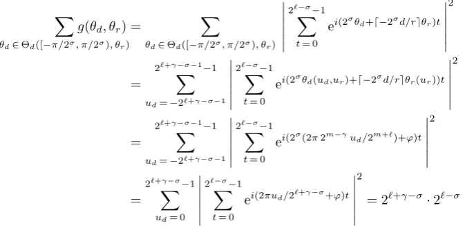
As was stated above, we seek a closed form approximation toρ(θd, θr, e) summed
over allrgroup elementsy= [e]g∈G. Hereinafter, we denote this probability
P(θd, θr) = r−1
X
e= 0
ρ(θd, θr, e)
= 1
22(m+2`)
r−1
X
e= 0
2` −1 X
b= 0
eiθdb
d(2m+`−(e+bd))/re−1
X
nr=d−(e+bd)/re
eiθrnr
2 , (6)
3.1
Preliminaries
To gain some intuition, we writeρ(θd, θr, e) as
1 22(m+2`)
2` −1 X
b= 0
ei(θdb+θrd−(e+bd)/re)
d(2m+`
−(e+bd))/re−d−(e+bd)/re−1
X
nr= 0
eiθrnr
2
and note that there are two obstacles to placing this expression on closed form: Firstly, the summation interval in the inner sum overnr depends on the
sum-mation variablebof the outer sum. Secondly, the exponent of the summand in the outer sum overbcontains a rounding operation that depends onb.
By using that(2m+`−(e+bd))/r− d−(e+bd)/re ≈
2m+`/r we may re-move the dependency between the inner and outer sums, and by using thatd−(e+bd)/re ≈ −(e+bd)/rwe may remove the rounding operation.
By making these two approximations, and by adjusting the phase, we may derive an approximation toρ(θd, θr, e) that is independent ofe, enabling us to sum
ρ(θd, θr, e) over thervalues ofe, corresponding to thergroup elementsy= [e]g∈
G, simply by multiplying byr. This yields
P(θd, θr)≈
r
22(m+2`)
2` −1 X
b= 0
ei(θd−θrd/r)b
2
d2m+`/re−1
X
nr= 0
eiθrnr
2 = r
22(m+2`)
ei2`(θd−θrd/r)−1
ei(θd−θrd/r)−1
2
eid2m+`/reθr−1
eiθr−1
2 (7)
where we furthermore need to assume in (7) thatθd−θrd/r6= 0 and θr6= 0.
This closed form approximation captures the general characteristics of the prob-ability distribution induced by the quantum algorithm. However, it is seemingly non-trivial to derive a good bound for the error in this approximation.
In what follows, we use techniques similar to those employed above to derive an error-bounded closed form approximation to ρ(θd, θr, e) such that the error is
negligible in the regions of the plane where the probability mass is concentrated. As was the case above, we will find that the error-bounded approximation of
ρ(θd, θr, e) is independent of e, enabling us to approximate P(θd, θr) simply by
multiplying the closed form approximation toρ(θd, θr, e) byr.
3.1.1 Constructive interference
Before we proceed to develop the closed form approximation, we note that for a fixed problem instance and fixed e, the sums in ρ(θd, θr, e) are over a constant
number of unit vectors in the complex plane. For such sums, constructive inter-ference arises when all vectors point in approximately the same direction.
In regions of the plane whereθrandθd−d/r θrare both small, we hence expect
constructive interference to arise. The probability mass is expected to concentrate in regions where constructive interference arises, and where the concentration of pairs (θd, θr) yielded by the integers pairs (j, k) is great.
In what follows, we therefore seek to derive a closed form approximation to
ρ(θd, θr, e), and an associated bound on the error in the approximation, such that
a
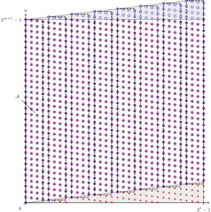
b 2`−1 2m+`−1
0 A
Fig. 1: The lattice La,b for σ = 2. All red filled points are in R. The regionAand its translated replicas are drawn as dashed rectangles. All blue outlined points are inAor in one of its replicas. The gray triangles outline the points that are inAor one of its replicas, but not inR, and vice versa.
3.2
Closed form approximation with error bounds
To derive a closed form approximation toρ(θd, θr, e), we first observe that the sums
in the expression forρ(θd, θr, e) may be regarded as sums over the points in a region
R in a latticeLa,b, as is illustrated in Fig. 1. Note that this figure also contains other elements to which we shall return as the analysis progresses.
Definition 3.1. Let La,b be the lattice spanned by (d,1) and(r,0) so that the set
of points in La,b is given by(a, b) =b(d,1) +nr(r,0) for integersb andnr.
Definition 3.2. LetRbe the region inLa,b where0≤a <2m+` and0≤b <2`.
Definition 3.3. Let
SR= |sR|
2
22(m+2`) where sR=
X
(a,b)∈ R
exp
2πi
2m+`(aj+ 2 mbk)
.
Proof. The points inRare given by (a, b) =b(d,1) +nr(r,0), for 0≤b <2` and
nr on (2) so that 0≤a=e+bd+nrr <2m+`, which implies that
SR = 1 22(m+2`)
2`−1
X
b= 0
d(2m+`
−(e+bd))/re−1
X
nr=d−(e+bd)/re
exp
2πi
2m+`(nrrj+b(dj+ 2 mk))
2
= 1
22(m+2`)
2`−1
X
b= 0
eiθdb
d(2m+`
−(e+bd))/re−1
X
nr=d−(e+bd)/re
eiθrnr
2
=ρ(θd, θr, e)
by the preliminary analysis in section 3 and so the claim follows.
In what follows, we derive a closed form approximation to ρ(θd, θr, e) = SR,
and an associated error bound, in three steps.
3.2.1 Preliminaries
Before proceeding as outlined above, we first introduce some preliminary claims.
Claim 3.2. Foru, v∈Cand∆ =u−v it holds that
|u|2− |v|2
≤2|u| |∆|+|∆|2.
Proof. First verify that
|u|2− |v|2=|u|2− |u−∆|2=uu−(u−∆)(u−∆)
=uu−(u−∆)(u−∆) =u∆ +u∆− |∆|2
where the overlines denote complex conjugates. This implies that
|u|2− |v|2
≤ |u| |∆|+|u| |∆| +|∆|2= 2|u| |∆|+|∆|2
and so the claim follows.
Claim 3.3. |eiφ−1| ≤ |φ|for any φ∈R.
Proof. It suffices to show that|eiφ−1|2= 2(1−cosφ)≤φ2 from which the claim
follows as cosφ≥1−φ2/2 for anyφ∈R.
3.2.2 Bounding |sR|
Before proceeding to the first approximation step, we furthermore bound |sR|in this section, as this bound is needed in the following analysis.
Lemma 3.1. The sum sR is bounded by|sR| ≤22`+1.
Proof. By Claim 3.1 the sum
sR=
2`−1
X
b= 0
eiθdb
d(2m+`
−(e+bd))/re−1
X
nr=d−(e+bd)/re
eiθrnr
where the outer sum over bis over 2` values and the inner sum overn
r is over at
Claim 3.4. For∆ =(2m+`−(e+bd))/r− d−(e+bd)/re, it holds that
∆ =
2m+`/r
−td=
2m+`/r
+tb ≤2`+1 for some td, tb∈ {0,1}.
Proof. For somef1, f2∈[0,1), it holds that
∆ =2m+`/r−f1+d−(e+bd)/re −f2− d−(e+bd)/re
=
2m+`/r
+d−(e+bd)/re − d−(e+bd)/re+d−f1−f2e
wheretd=d−f1−f2e=− bf1+f2c ∈ {0,1} asf1+f2∈[0,2). Analogously,
∆ =
2m+`/r
+f10+d−(e+bd)/re −f2− d−(e+bd)/re
=
2m+`/r
+d−(e+bd)/re − d−(e+bd)/re+df10−f2e
again for somef10 ∈[0,1), wheretb=df10−f2e ∈ {0,1}as f10−f2∈(−1,1).
Finally, recall that r≥ 2m−1. Hence, it follows that 2m+`/r ≤2`+1, so ∆ =
2m+`/r−td≤2`+1, and so the claim follows.
3.2.3 Approximating SR by SATA
In the first approximation step, we approximate SR by summing the points in a small regionAinR, and then replicating and translating the points inA, and the associated sum over these points, so as to approximately coverR, see Fig. 1.
Definition 3.4. Let A be the region in La,b where0≤a <2m+` and0 ≤b <2σ
forσan integer parameter selected on 0< σ < `.
Definition 3.5. Let
SA= |sA|
2
22(m+2`) where sA=
X
(a,b)∈ A
exp
2πi
2m+`(aj+ 2 mbk)
.
Claim 3.5.
SA= 1 22(m+2`)
2σ −1 X
b= 0
eiθdb
d(2m+`−(e+bd))/re−1
X
nr=d−(e+bd)/re
eiθrnr
2 .
Proof. The points in Aare given by (a, b) =b(d,1) +nr(r,0) for 0≤b <2σ and
nr on (2) so that 0≤a=e+bd+nrr <2m+` which implies that
SA= 1 22(m+2`)
2σ −1 X
b= 0
d(2m+`
−(e+bd))/re−1
X
nr=d−(e+bd)/re
exp
2πi
2m+`(nrrj+b(dj+ 2 mk))
2 = 1
22(m+2`)
2σ−1
X
b= 0
eiθdb
d(2m+`
−(e+bd))/re−1
X
nr=d−(e+bd)/re
eiθrnr
2
To replicate and translate the points inAso as to approximately cover R, we furthermore introducetAandTA, as defined below:
Definition 3.6. Let
TA=|tA|2 where tA=
2`−σ−1
X
t= 0
ei(θd2σ+θrd−2σd/re)t.
The error when approximatingSR bySATA may now be bounded as follows:
Lemma 3.2. The error when approximating sR by sAtA is bounded by
|sR−sAtA| ≤22`−σ+1.
Proof. The exponential sum tA replicates and translates the partial sum over A
so as to approximately cover Ras is illustrated in Fig. 1. Every time the region is replicated, it is translated by ei(θd2σ+θrd−2σd/re). This exponential function may
be easily seen to correspond to a vector inLa,b. The error that arises whensR is approximated bysAtAis hence due to points that are inRbut excluded from the sum, and conversely to points not inRthat are erroneously included in the sum. Hereinafter these points will be referred to as the erroneous points.
The erroneous points fall within the two gray triangles in Fig. 1. Both triangles are of horizontal length 2` and vertical side length 2`−σ(2σdmodr), as the region
Ais replicated and translated 2`−σ times in total, and as it is shifted horizontally by 2σ and vertically by 2σdmodr every time it is translated.
To upper-bound the number of lattice points in each triangle, note that the lattice points are on 2`vertical lines, evenly separated horizontally by a distance of one. The points on each vertical line are evenly separated vertically by a distance of
r, with varying starting positions on each line. For h(b) = 2`−σ(2σdmod r)(b/2`) the height of each triangle atb, we have that at most
N(b) = 1 +bh(b)/rc ≤1 +h(b)
r = 1 +
2σdmod r
r b
2σ ≤1 +
b
2σ
lattice points are then on the vertical line that cuts through the triangle at b, as may be seen by maximizing over all possible starting points. By summing N(b) over all 2` lines, we thus obtain an upper bound of
2`
−1
X
b= 0
N(b)≤2`+ 1 2σ
2`
−1
X
b= 0
b= 2`+ 1 2σ
2`(2`−1)
2 ≤2
2`−σ
on the number of points in each triangle, where we have used that 22`−σ−1 ≥2` as σ is an integer on 0 < σ < `. As there are two triangles, the total number of erroneous points is upper-bounded by 2·22`−σ = 22`−σ+1. Each erroneous point corresponds to a unit vector in the complex sum sR−sAtA, which implies
|sR−sAtA| ≤22`−σ+1, and so the lemma follows.
Lemma 3.3. The error when approximating SR by SATA is bounded by
Proof. By Claim 3.2, it holds that
|sR|2− |sAtA|2
≤2|sR| |sR−sAtA|+|sR−sAtA|2
≤2·22`+1·22`−σ+1+ 24`−2σ+2
≤3·24`−σ+2≤24(`+1)−σ
as |sR−sAtA| ≤22`−σ+1 by Lemma 3.2 and|sR| ≤22`+1 by Lemma 3.1. From the above, and Definitions 3.3, 3.5 and 3.6, we have that
|SR−SATA|=
|sR|2− |sAtA|2
22(m+2`) ≤
24(`+1)−σ 22(m+2`) = 2−
2m−σ+4
and so the lemma follows.
AstAis a geometric seriesTA=|tA|2may be placed on closed form. It remains
to derive a closed form approximation toSA in two more steps.
3.2.4 Approximating SA by SA0
In the second approximation step, we derive a closed form approximation to SA, by first approximating SA by the product SA0 of two sums, such that the leading sum may be placed on closed form, and such that the trailing sum may be placed on closed form by means of a third approximation step.
Definition 3.7. Let
SA0 = |s
0
A|
2
22(m+2`) where s
0
A=
2σ
−1
X
b= 0
ei(θdb+θrd−(e+bd)/re)
d2m+`/re−1
X
nr= 0
eiθrnr.
Lemma 3.4. The error when approximating sAby s0A is bounded by
|sA−s0A| ≤2σ.
Proof. AssA ands0A are sums of complex unit vectors, and as the sums differ by at most 2σ vectors, as may be seen by comparing the summation intervals using Claim 3.4, it follows that|sA−s0A| ≤2σ, and so the lemma follows.
Lemma 3.5. The sum s0Ais bounded by |s0A| ≤2`+σ+1.
Proof. In the expression fors0Ain Definition 3.7, the sum overbassumes 2σvalues and the sum over nrassumes at most 2`+1 values as the orderr≥2m−1.
Ass0Ais a sum of at most 2`+σ+1 complex unit vectors, it follows that|s0A| ≤
2`+σ+1, and so the lemma follows.
Lemma 3.6. The error when approximating SA bySA0 is upper-bounded by
|SA−SA0 | ≤2−2m−3`+2σ+3.
Proof. By Claim 3.2, it holds that
|sA|2− |s0A|2
≤2|s0A| |sA−s0A|+|sA−s0A|
2
≤2·2`+σ+1·2σ+ 22σ
as |sA−s0A| ≤2σ by Lemma 3.4 and|s0A| ≤2`+σ+1 by Lemma 3.5. From the above, and Definitions 3.5 and 3.7, we have that
|SA−SA0 |=
|sA|2− |s0A|2
22(m+2`) ≤
2`+2σ+3 22(m+2`) = 2
−2m−3`+2σ+3
and so the lemma follows.
The trailing sum inSA0 is the square norm of a geometric series. Hence, it may be trivially placed on closed form. Due to the rounding operation in the exponent, this approach is not valid for the leading sum; we need a third approximation step.
3.2.5 Approximating SA0 by SA00
For θd and θr such that the angles θdb+θrd−(e+bd)/re ≈ (θd−θrd/r)b in the
leading sum in SA0 are small for allb on 0≤b < 2σ, all 2σ terms in the sum are approximately one. In the third and final step of the approximation, we bound the error when simply approximating all terms in the leading sum by one.
Definition 3.8. Let
SA00 = |s
00 A|2
22(m+2`) where s00A= 2σ
d2m+`/re−1
X
nr= 0
eiθrnr.
Lemma 3.7. The difference between s0A ands00Ais upper-bounded by
|s0A−s00A| ≤2σ−1(|θd|+|θr|)|s00A|.
Proof. First observe that
|s0A−s00A|=
2σ −1 X
b= 0
ei(θdb+θrd−(e+bd)/re)−1
| {z }
|∆|
d2m+`/re−1
X
nr= 0
eiθrnr
.
By using Claim 3.3 and the triangle inequality, it follows that
|∆|=
2σ−1
X
b= 0
ei(θdb+θrd−(e+bd)/re)−1
≤
2σ−1
X
b= 0
e
i(θdb+θrd−(e+bd)/re)−1
≤
2σ
−1
X
b= 0
|θdb+θrd−(e+bd)/re |=
2σ
−1
X
b= 0
|θdb−θrb(e+bd)/rc |
≤(|θd|+|θr|)
2σ−1
X
b= 0
b≤(|θd|+|θr|)
2σ(2σ−1)
2 ≤2
2σ−1(|θ
d|+|θr|)
where we use that d−xe=− bxcandb(e+bd)/rc ≤b. To verify the latter claim, note thatf1=e/r∈[0,1) andf2=bd/r∈[0, b) ase, d∈[0, r). This implies that
b(e+bd)/rc=bf1+f2c ∈[0, b] asf1+f2∈[0, b+ 1).
By combining the above results, we now have that
|s0A−s00A| ≤22σ−1(|θd|+|θr|)
d2m+`/re−1
X
nr= 0
eiθrnr
= 2σ−1(|θd|+|θr|)|s00A|
and so the lemma follows.
Lemma 3.8. The error when approximating SA0 bySA00 is upper-bounded by
|S0A−SA00| ≤2σ−1(|θd|+|θr|) 2 + 2σ−1(|θd|+|θr|)S00A.
Proof. By Claim 3.2, it holds that
|s0A|2− |s00A|2
≤2|s00A| |s0A−s00A|+|s0A−s00A|
2
≤2·2σ−1(|θd|+|θr|)|s00A|2+ 22(σ−1)(|θd|+|θr|)2|s00A|2
= 2σ−1(|θd|+|θr|) 2 + 2σ−1(|θd|+|θr|)|s00A|
2
as |s0A−s00A| ≤2σ−1(|θd|+|θr|)|s00A|by Lemma 3.7.
From the above, and Definitions 3.7 and 3.8, we have that
|SA0 −SA00|=
|s0A|2− |s00A|2
22(m+2`)
≤2σ−1(|θd|+|θr|) 2 + 2σ−1(|θd|+|θr|)SA00
and so the lemma follows.
This yields an approximationSA00 to SA0 that may be placed on closed form.
3.2.6 Main approximability result
By combining the above results, the main approximability result follows:
Theorem 3.1. The probability P(θd, θr) of observing a specific pair (j, k) with
angle pair (θd, θr), summed over ally∈G, may be approximated by
e
P(θd, θr) =
22σr
22(m+2`)
2`−σ−1
X
t= 0
ei(θd2σ+θrd−2σd/re)t
2
d2m+`/re−1
X
nr= 0
eiθrnr
2
= 2
2σr
22(m+2`)
ei(θd2σ+θrd−2σd/re) 2`−σ−1
ei(θd2σ+θrd−2σd/re)−1
2
eiθrd2m+`/re −1
eiθr−1
2
assumingθd2σ+θrd−2σd/re 6= 0andθr6= 0when placing the expression on closed
form. The approximation error|P(θd, θr)−Pe(θd, θr)| ≤˜e(θd, θr)where
˜
e(θd, θr)≤
24 2m+σ +
23 2m+`+
2σ
2 (|θd|+|θr|)
2 +2
σ
2 (|θd|+|θr|)
e
P(θd, θr).
Proof. The probabilityρ(θd, θr, e) of observing a specific pair (j, k), with angle pair
(θd, θr), and some group elementy= [e]g∈G, is SR by Claim 3.1.
The error when approximatingSR bySATAis bounded by
|SR−SATA| ≤2−2m−σ+4
by Lemma 3.3. The error when approximatingSATA bySA0 TAis bounded by
by Lemma 3.6. The error when approximatingSA0 TA bySA00TAis bounded by
|S0ATA−SA00TA| ≤2σ−1(|θd|+|θr|) (2 + 2σ−1(|θd|+|θr|))SA00TA
by Lemma 3.8. By the triangle inequality
|SR−SA00TA|=|(SR−SATA) + (SATA−SA0 TA) + (SA0 TA−SA00TA)| ≤ |SR−SATA|+TA|SA−SA0 |+TA|S0A−SA00|.
Neither of these three error terms, nor the expression for S00ATA, depend on e. Hence, we may sum over all relementsy= [e]g∈Gby multiplying byr.
It therefore follows thatPe(θd, θr) =rSA00TA is an approximation to P(θd, θr),
and that the error that arises in this approximation is bounded by
˜
e(θd, θr)≤r|SR−SATA|+rTA|SA−SA0 |+rTA|SA0 −SA00| ≤2−2m−σ+4r+ 2−2m−3`+2σ+3rTA+
2σ−1(|θd|+|θr|) (2 + 2σ−1(|θd|+|θr|))rSA00TA
≤ 2
4
2m+σ +
23 2m+` +
2σ
2 (|θd|+|θr|)
2 + 2
σ
2 (|θd|+|θr|)
e
P(θd, θr)
where we use thatr <2m, and thatTA≤22(`−σ)as it is the square norm of a sum of 2`−σ unit vectors by Definition 3.6, and so the theorem follows.
In appendix C we demonstrate the soundness of this approximation.
4
The distribution of pairs
(
α
d, α
r)
In this section, we identify and count all pairs (j, k) that yield (αd, αr) and analyze
the distribution and density of pairs (αd, αr) in the plane.
Definition 4.1. An argument pair(αd, αr)is said to be admissible if there exists
an integer pair (j, k), for j on0≤j <2m+` andkon 0≤k <2`, such that
αd={dj+ 2mk}2m+` and αr={rj}2m+`.
Definition 4.2. Letκd denote the greatest integer such that2κd dividesd, and let
κr denote the greatest integer such that2κr divides r.
Definition 4.3. LetLαbe the lattice generated by the rows in
δr 2κr
2m−γ 0
where δr=d
r
2κr
−1
mod 2m−γ
andγ= max(0, κr−(`+κd)).
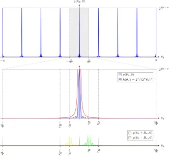
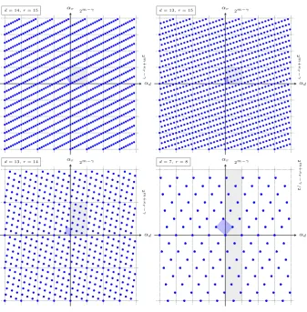
Lemma 4.1. The admissible argument pairs (αd, αr) are vectors in the region
−2m+`−1 ≤ αd, αr < 2m+`−1 in Lα. There are 2m+2`−κr+γ distinct admissible
d= 14, r= 15
αd
αr 2m−γ
2
m
+
κ
r
−
γ
d= 13, r= 15
αd
αr 2m−γ
2
m
+
κ
r
−
γ
d= 13, r= 14
αd
αr
2m−γ
2
m
+
κ
r
−
γ
d= 7, r= 8
αd
αr
2m−γ
2
m
+
κ
r
−
γ
/
2
Fig. 2: The distribution of admissible arguments (αd, αr) in the region where
−2m+`−1≤α
d, αr<2m+`−1form= 4 and`= 3, and example combinations of d and r, as indicated. The lattice may be constructed by replicating the fundamental parallelogram (blue) or a rectangle (gray) of size 2m−γ×
2m+κr−γ .
Proof. Asαr≡rj (mod 2m+`), the set of integers j that yieldαrare given by
j≡ αr
2κr
r
2κr
−1
+ 2m+`−κrt
r (mod 2m+`)
fortr an integer on 0≤tr<2κr. Asαd≡dj+ 2mk (mod 2m+`), we need
αd≡d
α
r
2κr
r
2κr
−1
+ 2m+`−κrt r
+ 2mk
≡ αr
2κrd
r
2κr
−1
+ 2m+`−κr+κd dtr
2κd
| {z }
A
+ 2mk
| {z }
B
(mod 2m+`) (8)
forkan integer on 0≤k <2`, to ensure compatibility. As 2m−γis the largest power
of two to divide both 2mand 2m+`−κr+κd, by the definition of γ, the congruence
Astr andkrun through all pairwise combinations, the set of 2`+κr arguments
αd generated by (8) is equal to that generated by
αd≡
αr
2κrd
r
2κr
−1
+ 2m−γtγ (9)
≡ αr
2κr
d r
2κr
−1
mod 2m−γ
+ 2m−γt0γ (mod 2m+`) (10)
as tγ, or equivalentlyt0γ, runs through all integers on 0≤tγ, t0γ <2`+κr.
To go from (8) to (9), first note that B runs through all values in [2m,2m+`). Ifγ= 0, term A introduces multiplicity by repeating the sequence generated by B with various offsets. These offsets are of no significance to this analysis, as we only account for which values occur in the set and with what multiplicity.
Ifγ >0, term A runs through all values in [2m−γ,2m−γ+κr). Asκ
r≥γ when
γ >0, term A runs all values in the subrange [2m−γ,2m). When A assumes values greater than or equal to 2m, it introduces multiplicity by repeating the sequence of all values on [2m−γ,2m+`) generated by A and B with various offsets.
This implies that (A + B) mod 2m+`runs through all 2m+`/2m−γ= 2`+γvalues on [2m−γ,2m+`) with multiplicity 2`+κr/2`+γ = 2κr−γ, and this is exactly what is
stated in (9). To go from (9) to (10) is trivial.
As there are 2m+2` admissible argument pairs, and as each pair occurs with multiplicity 2κr−γ, there are 2m+2`−κr+γ distinct admissible argument pairs.
The latticeLα is constructed from (10), as the admissibleαr are multiples of
2κr, and as the admissibleα
d≡(αr/2κr)δr+ 2m+γt0γ (mod 2m+`), in the region
of the plane where−2m+`−1≤αd, αr<2m+`−1, and so the lemma follows.
In Fig. 2 the distribution of arguments in the region of the plane where−2m+`−1≤
αd, αr<2m+`−1 is depicted for various combinations of parameters.
4.1
Pairs
(
j, k
)
yielding
(
α
d, α
r)
In this section we identify all pairs (j, k) that yield (αd, αr).
Lemma 4.2. The set of integer pairs (j, k), for j on 0 ≤ j < 2m+` and k on
0≤k <2`, that yield the admissible argument pair(αd, αr) is given by
j=
α
r
2κr
r
2κr
−1
+ 2m+`−κrt r
mod 2m+` and k=αd−dj
2m mod 2 `
astr runs through all integer multiples of2γ on0≤tr<2κr.
Proof. Asαr≡rj (mod 2m+`), solving for j yields
j= αr 2κr
r
2κ r
−1
+ 2m+`−κrt r
!
mod 2m+`
fortr an integer 0≤tr<2κr.
Asαd ≡dj+ 2mk (mod 2m+`), for compatibility 2m must divide 2m+`−κrdtr
for all tr6= 0. As 2m+`+κd−κr is the greatest power of two to divide 2m+`−κrd, it
4.2
The density of pairs
(
α
d, α
r)
In this section we analyze the density of pairs (αd, αr) in the argument plane.
Claim 4.1. The density of admissible argument pairs in the region of the plane
where−2m+`−1≤αd, αr<2m+`−1 is2−m when accounting for multiplicity.
Proof. There are 2m+2` admissible (αd, αr), when accounting for multiplicity, in
the region where−2m+`−1≤αd, αr<2m+`−1. This region is of area 22(m+`). The
density is hence 2m+2`/22(m+`)= 2−m, and so the claim follows.
To construct the histogram for the probability distribution, the argument plane is divided into small rectangular subregions. The below lemma bounds the error when approximating the density in such subregions by 2−m.
Lemma 4.3. Let D be the density of admissible argument pairs (αd, αr), when
accounting for multiplicity, in a rectangleR of area Aand circumference C in the region where −2m+`−1≤α
d, αr<2m+`−1 of the plane. Then
D− 1
2m
≤2κr−γ 2Cλ2+ 4 (2λ2)
2
A detLα =
2Cλ2+ 4 (2λ2)2
2mA
forλ1 the norm of the shortest non-zero vector w1∈Lα, and λ2 the norm of the
shortest non-zero vector w2∈Lαthat is linearly independent to w1.
Proof. By Lemma 4.1, the admissible argument pairs (αd, αr) are vectors inLαin
the region of the argument plane where−2m+`−1≤αd, αr<2m+`−1. Each
admis-sible argument pair occurs with multiplicity 2κr−γ.
The fundamental parallelogram in Lα contains a single lattice vector. It is spanned by w1 and w2, and has area detLα=λ2|w⊥|= 2m+κr−γ, wherew⊥ is
the component inw1perpendicular tow2. This impliesλ2≥λ1≥ |w⊥|.
To bound the number of argument pairs (αd, αr) ∈ R, we lower- and
upper-bound the number of fundamental parallelograms that can at most fit into R, as described below, paying particular attention to the border areas:
To upper-bound the number of vectors inR, we extend each side ofRby 2λ2
length units, to ensure that any parallelogram that is only partly inR is included in the count, and divide the area of the resulting rectangle by the area of the fundamental parallelogram. This yields (A+ 2Cλ2+ 4 (2λ2)2)/detLα.
Conversely, to lower-bound the number of vectors in R, we retract each side of R by 2λ2 length units, to ensure that all parallelograms that are only partly
in the rectangle are excluded from the count, and divide the area of the resulting rectangle by detLα. This yields (A−2Cλ2+ 4 (2λ2)2)/detLα.
By combining the upper and lower bounds, dividing by the areaA of R, and multiplying by 2κr−γ to account for multiplicity, the lemma follows.
For known d and r, Lemma 4.3 above provides a bound on the error when approximating the density in a rectangle inLαby 2−masλ2may then be computed.
To bound the error for general problem instances, and whendandrare unknown, we introduce the following less tight lemma:
Lemma 4.4. Let D be the density of admissible argument pairs (αd, αr), when
αr directions, respectively, in the region where−2m+`−1≤αd, αr<2m+`−1 of the
argument plane. Then
D− 1
2m
≤ 2
κr
2ml r
+ 1
2γl d
+ 1
ldlr
.
Proof. By Lemma 4.1, the admissible argument pairs are vectors inLα.
The vectors in Lα are on horizontal lines (for fixed αr) evenly separated by
a vertical distance of 2κr. The number of such lines that intersect the rectangle
is upper-bounded by blr/2κrc+ 1≤lr/2κr + 1 and lower-bounded byblr/2κrc ≥
lr/2κr −1 as may be seen by positioning the rectangle to maximize or minimize
the number of lines that intersect the rectangle.
On each line, the vectors inLα are evenly spaced by a distance of 2m−γ with varying starting positions. The number of vectors in Lα that fall within the rect-angle on each line is upper-bounded by bld/2m−γc+ 1≤ld/2m−γ + 1 and
lower-bounded by bld/2m−γc ≥ ld/2m−γ −1, when not accounting for multiplicity, as
may be seen by positioning the line to maximize or minimize the number of vectors that fall within the rectangle.
Hence the number of lattice vectors in the rectangle is upper-bounded by
2κr−γ(l
r/2κr+ 1)(ld/2m−γ+ 1) =ldlr/2m+ld2κr/2m+lr/2γ+ 1
and lower-bounded by
2κr−γ(l
r/2κr−1)(ld/2m−γ−1) =ldlr/2m−ld2κr/2m−lr/2γ+ 1
as each vector corresponds to a pair that occurs with multiplicity 2κr−γ.
By combining the above bounds, and dividing by the arealdlr of the rectangle,
the lemma follows.
For unknown d and r, the above lemma provides an error bound, assuming only some bounds on the parameters κr and γ. Asymptotically, the error in the
approximation tends to zero as the side lengths of the rectangle tend to infinity. For rectangular subregions of specific dimensions, it may furthermore be shown that the error is zero, as is demonstrated in the following lemma:
Lemma 4.5. The density of admissible argument pairs in a rectangle of side lengths
positive integer multiples of 2m−γ and2m−γ+κr inα
d andαr, respectively, in the
region where −2m+`−1 ≤ αd, αr < 2m+`−1 of the argument plane, is 2−m when
accounting for multiplicity.
Proof. By Lemma 4.1, the admissible arguments are vectors inLαin the region of
the argument plane where−2m+`−1≤α
d, αr<2m+`−1.
From the definition of Lα in Lemma 4.1, it follows that the lattice is cyclic with period 2m−γ in αd and 2m−γ+κr in αr. This is illustrated in Fig. 2 where
rectangular regions of these dimensions are highlighted in gray. The highlighted regions all extend from the origin in Fig. 2 but the starting point may of course be arbitrarily selected. This implies that the lattice Lα may be generated by replicating and translating any rectangle of side lengths positive multiples of 2m−γ and 2m−γ+κr in α
d and αr, respectively, see Fig. 2, throughout the plane. The
sgn(
α
d
)
log
2
(
|
α
d
|
)
sgn(αr) log2(|αr|)
m
−m
m
−m
η
d dη
+
1
/
2
ν
η
d
+
2
/
2
ν
η
d
+
1
ηr ηr+ 1/2ν ηr+ 2/2ν ηr+ 1
2
η
r
+(
ξ
r
+1)
/
2
ν
2
η
r
+
ξ
r
/
2
ν
αr
αd
2
η
d
+
ξ
d
/
2
ν
2
η
d
+(
ξ
d
+1)
/
2
ν
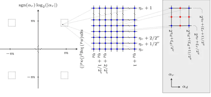
Fig. 3: The subdivision of the plane into regions and subregions. The gray box illustrates Simpson’s rule applied to a subregion. The probability is computed in the blue corner points, the four red border midpoints and the red centerpoint.
The number of rectangles that fit in the region when replicated and translated cyclically is 22(m+`)/22(m−γ)+κr = 22(`+γ)−κr as the area of the region is 22(m+`)
and the area of the rectangle is 22(m−γ)+κr. The total number of lattice vectors
in the region is 22m+`, so each rectangle contains 2m+2`/22(`+γ)−κr = 2m−2γ+κr
vectors when accounting for multiplicity.
By dividing by the rectangle area, we see that the density of points in each rectangle is 2m−2γ+κr/22(m−γ)+κr = 2−m, and so the lemma follows.
5
Simulating the quantum algorithm
In close analogy with [5], we now proceed to construct a high-resolution histogram for the probability distribution induced by the quantum algorithm, for given d
andr, and to sample it to simulate the quantum algorithm.
5.1
Constructing the histogram
Except for the fact that the probability distribution is two-dimensional, and that we need to account for the closed form expression being an approximation, we exactly follow [5] to construct the high-resolution histogram: We subdivide the ar-gument plane into regions and subregions, and integrate the closed form probability approximation and the associated error bound numerically in each subregion.
First, we subdivide each quadrant of the argument plane into (30 +µ)2 rect-angular regions where µ = min(`−2,11). Each region thus formed is uniquely identified by (ηd, ηr)∈Z2 by requiring that for all (αd, αr) in the region
2|ηd|≤ |α
d| ≤2|ηd|+1 and 2|ηr|≤ |αr| ≤2|ηr|+1,
and furthermore sgn(αd) = sgn(ηd) and sgn(αr) = sgn(ηr), where ηd and ηr are
Then, we subdivide each region into rectangular subregions identified by an integer pair (ξd, ξr) by requiring that for all (αd, αr) in the subregion
2|ηd|+ξd/2ν ≤ |α
d| ≤2|ηd|+(ξd+1)/2 ν
and 2|ηr|+ξr/2ν ≤ |α
r|<2|ηr|+(ξr+1)/2 ν
where 0≤ξd, ξr<2ν forν∈ {6,7,8,9}a resolution parameter adaptively selected
as a function of the probability mass and variance in each region.
For each subregion, we compute the approximate probability mass contained within the subregion, and an associated error bound, by applying Simpson’s rule in two dimensions, followed by Richardson extrapolation to cancel the linear error term, and division by 2mto account for the density of pairs.
Simpson’s rule is hence applied 22ν(1+22) times in each region. Each application requires the approximate probability and associated error bound to be computed in up to nine points, for which purpose we use the closed form expressions in Theorem 3.1, with σadaptively selected to suppress the bounded error.
The optimal σ may be found by searching exhaustively. A computationally more efficient method for selectingσis to use the heuristic in appendix C.5.3. We use the heuristic in all cases except when s is large in relation to m causing the error in the close-form approximation to be large. For suchmandswe accept an extra computational burden to get slightly betterσand slightly smaller errors.
In order to save space when storing the histogram, we discard regions that capture insignificant shares of the probability mass. Note furthermore that for
m and s such that the total error in the closed form approximation is large, the error may often be reduced at the expense of capturing a smaller fraction of the probability mass by simply discarding selected regions where the error is large. The errors we report in this paper are without accounting for such additional filtering. Note that this method of constructing the histogram assumesκd andκr to be
small in relation to m. Note also that it follows from section 4.2 that it is sound to approximate the density by 2−min the four regions of interest in the plane. For themandsthat we consider, the error in the density approximation is negligible.
5.2
Understanding the probability distribution
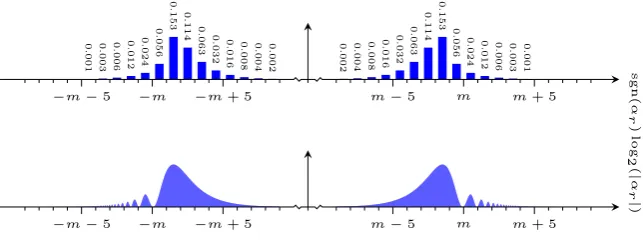
To illustrate the distribution that arises, a histogram is plotted in the signed loga-rithmic argument plane in Fig. 4 form= 2048 ands= 30, and fordandrselected as explained in section 7.3. It captures approximately 99.99% of the probability mass. The total approximation error is less than 10−3.
The histogram plotted in Fig. 4 captures the general characteristics of the prob-ability distribution. Varyingdandron the interval 2m−1< d < r <2m, fordandr
not divisible by large powers of two, in general only slightly affects the distribution. Scaling mandshas virtually no effect on the distribution.
The probability mass is located in the regions where (|αd|,|αr|)∼(2m,2m),
whereas for random outputs the arguments would be of size ∼ 2m+`. Hence, a single run yields∼`∼m/sbits of information ondandr, respectively.
The distribution is symmetric, in that the top right and lower left quadrants are mirrored, as are the top left and lower right quadrants. It hence suffices to compute only two quadrants to construct the histogram. To see why this is, note that flipping the sign of both arguments in the expression for Pe(θd, θr) in Theorem 3.1 has no
m−5 m m+ 5
−m−5 −m −m+ 5
sgn ( α d ) log 2 ( | α d | ) m − 5 m m + 5 − m − 5 − m − m + 5
sgn(αr) log2(|αr|)
0.127 0.127 0.112 0.112 0.079 0.079 0.047
0.047 0.042 0.042 0.024 0.024 0.021 0.021 0.012 0.012 0.011 0.011 0.006 0.006 0.005 0.005 0.003 0.003 0.003 0.003 0.002 0.002 0.001 0.001
m−5 m m+ 5
−m−5 −m −m+ 5
m−5 m m+ 5
−m−5 −m −m+ 5
sgn ( α d ) log 2 ( | α d | ) 0.153 0.153 0.114 0.114 0.063 0.063 0.056 0.056 0.032 0.032 0.024 0.024 0.016 0.016 0.012 0.012 0.008 0.008 0.006 0.006 0.004 0.004 0.003 0.003 0.002 0.002 0.001 0.001 m − 5 m m + 5 − m − 5 − m − m + 5 m − 5 m m + 5 − m − 5 − m − m + 5
sgn(αr) log2(|αr|)
Fig. 4: The probability distribution for general discrete logarithms computed as in section 5.1 form= 2048,s= 30, anddandrselected as in section 7.3. To facilitate printing, the resolution has been reduced in this figure.
0.127 0.127 0.112 0.112 0.079 0.079 0.047
0.047 0.042 0.042
0.024
0.024 0.021 0.021 0.012
0.012 0.011 0.011 0.006
0.006 0.005 0.005 0.003
0.003 0.003 0.003 0.002
0.002 0.001 0.001
m−5 m m+ 5
−m−5 −m −m+ 5
m−5 m m+ 5
−m−5 −m −m+ 5
sgn( α d ) log 2 ( | α d | )
Fig. 5: The probability distribution for short discrete logarithms computed as in appendix B from the closed form expression in [5], for m= 2048 and
the concentration of probability mass in the top right and lower left quadrants, and in the tail along the diagonal in Fig. 4 whereθd2σ+θrd−2σd/reis small.
The marginal distribution along theαd axis is virtually identical to the
prob-ability distribution induced by dwhen regarded as a short discrete logarithm, see [5] and Fig. 5 for comparison. Analogously, the marginal distribution along theαr
axis in Fig. 4 is virtually identical to the distribution induced byrwhen performing order finding, see appendix A and Fig. 6 for comparison. In appendix D we show this analytically by summing Pe(θd, θr) over all admissibleθd.
This implies that the lattice-based post-processing algorithm introduced in [5] may be used to solve sets of pairs (j, k) for both short and general d, with mi-nor modifications, see section 6.1. An analogous lattice-based algorithm may be developed to solve sets of integersj forr, see section 6.2.
5.3
Sampling the probability distribution
Except for the fact that the probability distribution is two-dimensional, we exactly follow [5] to sample the distribution: To sample an argument pair (αd, αr), we first
sample a subregion and then sample (αd, αr) from this subregion.
To sample the subregion, we first order all subregions in the histogram by prob-ability, and compute the cumulative probability up to and including each subregion in the resulting ordered sequence. Then, we sample a pivot uniformly at random from [0,1), and return the first subregion in the ordered sequence for which the cu-mulative probability is greater than or equal to the pivot. Note that this procedure may fail: This occurs if the pivot is greater than the total cumulative probability.
To sample an argument pair (αd, αr) from the subregion, we first sample a point
(α0d, α0r)∈Z2 uniformly at random from the subregion. Then, we map (α0d, α0r) to
the closest admissible argument pair (αd, αr) ∈Lα by reducing the basis for Lα
given in Definition 4.3 and applying Babai’s algorithm [1].
To sample an integer pair (j, k) from the distribution, we first sample (αd, αr)
as described above, and then sample (j, k) uniformly at random from the set of all integer pairs (j, k) yielding (αd, αr) using Lemma 4.2. More specifically, we first
sample an integer tr uniformly at random from the set of all admissible values for
trand then compute (j, k) from (αd, αr) andtr as described in Lemma 4.2.
6
The classical post-processing algorithms
In this section, we describe how d and r are classically recovered from a set
{(j1, k1), . . . ,(jn, kn)}of pairs produced by performingnindependent runs.
6.1
Recovering
d
from a set of
n
pairs
To recoverd, we exactly follow [5], and use the set ofnpairs to form a vector
and aD-dimensional integer lattice Lj with basis matrix
j1 j2 · · · jn 1
2m+` 0 · · · 0 0
0 2m+` · · · 0 0
..
. ... . .. ... ...
0 0 · · · 2m+` 0
whereD=n+ 1. For some constantsm1, . . . , mn∈Z, the vector
ujd= ({dj1}2m+` +m12m+`, . . . ,{djn}2m+`+mn2m+`, d)∈Lj
is such that the distance
Rd=|ujd−v k d|=
v u u t
n
X
i=1
{dji}2m+` +mi2m+`− {−2mki}2m+`
2
+d2
=
v u u u t
n
X
i=1
{dji+ 2mki}22m+`
| {z }
α2
d,i
+d2 =
v u u t
n
X
i=1
α2
d,i+d2.
To recoverd, it hence suffices to findujdby enumerating all vectors inLjwithin a D-dimensional hypersphere of radiusRd centered onvkd. Its volume is
VD(Rd) =
πD/2
Γ D2 + 1R
D d
where Γ is the Gamma function, whilst the fundamental parallelepiped inLj, that by definition contains a single lattice vector, is of volume detLj= 2(m+`)n.
Heuristically, the hypersphere is hence expected to contain approximatelyvd=
VD(Rd)/ detLj lattice vectors. The exact number depends on the placement of
the hypersphere inZD, and on the shape of the fundamental parallelepiped inLj.
6.1.1 Estimating the minimum n required to solve ford
The radiusRddepends on (ji, ki) viaαd,ifor 1≤i≤n. For fixednand probability
qd, we exactly follow [5] and estimate the minimum radiusRed such that
Pr
Rd=
v u u t
n
X
i= 1
α2
d,i+d2≤Red
≥qd (11)
by samplingαd,ifrom the probability distribution. For details on how the estimate
is computed, see section 6.3. Equation (11) implies that
Pr
"
vd=
VD(Rd)
detLj ≤
VD(Red)
2(m+`)n
#
≥qd. (12)
This provides a heuristic bound on the number of lattice vectorsvd that at most
6.1.2 Selecting nand solving for d
A simple strategy when solving for d is to select n as described in section 6.1.1 such that vd is below a bound equal to the maximum number of vectors that it is
computationally feasible to enumerate with probabilityqd. This strategy minimizes
nat the expense of potentially computationally expensive post-processing. Another strategy is to select n such that vd <2 with probability qd. By the
heuristic, there is then only one vector in the hypersphere. In theory, this enables us to findujdwith probabilityqdby mappingvkd to the closest vector inLj without
enumerating vectors in Lj. In practice, however, the situation is now a bit more complicated as ujr = ({rj1}2m+`, . . . , {rjn}2m+`, r)∈Lj and this vector is short
in Lj by construction. This is because d+tris a solution to the general discrete logarithm problem for t an integer. To recover ujd, we therefore first map vkd to the closest vector in Lj, and then add or subtract small integer multiples of the shortest vector in the reduced basis to findujd. In essence, this amounts to reducing the last component of the vector closest to vk
d in Lj by r. However, as the last
component of the shortest vector in Lj may be a factor inr, see section 6.2.1, we
need to add and subtract multiples.
Note that this complication arises only for general discrete logarithms. It does not arise in [5] when post-processing short discrete logarithms, as the order then does not enter into the equation. Note furthermore that the fact that the order now does play a part may be leveraged in the post-processing, see the next sections.
6.1.3 Selecting nand solving for d by exhausting subsets
The greatest argument αd,i essentially determines the bound on Rd and hence
on vd. A plausible strategy is therefore to make n runs, but to independently
post-process all subsets of n−tpairs from the resulting npairs, fort a constant. To select nwhen using this strategy, we specify a bound B on the number of vectorsvd that we accept to enumerate in each lattice of dimensionn−t+ 1, and
follow section 6.1.1 to select the minimumnrespecting this bound with probability at leastqd, including only the smallestn−t argumentsαd,i when boundingRd.
With probabilityqd, the post-processing then requires at mostBlattice vectors
to be enumerated in at most nt
lattices of dimensionn−t+ 1. Note thatt must be limited to small values as the binomial coefficient grows rapidly int.
6.1.4 Optimizations when r is known
Note that whenris known, the argumentαr,i={rji}2m+` is known for 1≤i≤n,
andαr,i provides information onαd,i as the arguments are pairwise correlated.
When constructing subsets of n−t pairs from the n pairs (ji, ki), the pairs
should be included in ascending order sorted by |αr,i|. In general, pairs such that
|αr,i|exceed some bound may be rejected as large|αr,i|identify erroneous runs.
6.2
Recovering
r
from a set of
n
pairs
To recoverr, we instead use thatuj
r= ({rj1}2m+`, . . . ,{rjn}2m+`, r)∈Ljis a short
vector by construction. More specifically, we use thatuj
hypersphere inLj of radius
Rr=
ujr
=
v u u u t
n
X
i=1
{rji}22m+`
| {z }
α2
r,i
+r2 =
v u u t
n
X
i=1
α2
r,i+r2
centered at the origin. In close analogy with [5] and the previous section, we may recoveruj
rand hencerby enumerating all vectors in this hypersphere. Heuristically,
we expect the hypersphere to containvr=VD(Rr)/detLj lattice vectors.
This generalization was first hinted at in the pre-print of [4]. Furthermore, it is similar to the method employed by Seifert [18], where he uses what he refers to as simultaneous Diophantine approximation techniques to generalize Shor’s [19] continued fractions expansion-based post-processing to higher dimensions.
We prefer to describe the post-processing in terms of a shortest vector problem, as this gives us two lattice problems in the same latticeLj, and as we may re-use the above tools to estimate the number of runsnrequired to solve the problem.
6.2.1 Estimating the minimum n required to solve forr
The radiusRrdepends onji viaαr,i for 1≤i≤n. For fixednand probabilityqr,
we proceed in analogy with [5] and estimate the minimum radiusRersuch that
Pr
Rr=
v u u t
n
X
i=1
α2
r,i+r2≤Rer
≥qr (13)
by samplingαr,i from the probability distribution. For details on how the estimate
is computed, see section 6.3. Equation (13) implies that
Pr
"
vr=
VD(Rr)
detLj ≤
VD(Rer)
2(m+`)n
#
≥qr. (14)
This provides a heuristic bound on the number of lattice vectors vr that at most
have to enumerated to solve for r, and that holds with probability at leastqr.
6.2.2 Selecting nand solving for r
A simple strategy when solving for ris to select nsuch thatvr is below a bound
equal to the maximum number of vectors that it is computationally feasible to enu-merate with probabilityqr. This strategy minimizesnat the expense of potentially
computationally expensive post-processing.
Another strategy is to selectn such that vr <2 with probability qr. By the
heuristic, there is then only one lattice vector in the hypersphere. In theory, this enables us to find ujr with probabilityqr by computing the shortest vector inLj.
In practice, this is true in general whenris prime.
Assume the converse thatris composite. Lettbe a non-trivial divisor of both
r and αr,i for 1 ≤ i ≤ n. Then ujr/t ∈ Lj and |ujr/t| < |urj|, so ujr/t and r/t
are likely to be recovered by the algorithm instead ofujrandr. Forta non-trivial divisor of r, the probability of t also dividing αr,i for 1≤i≤n is approximately
(2κt/t)n, for 2κt the greatest power of two to dividet. This implies thatrmay be
6.3
Estimating
R
e
dand
R
e
rTo estimateRed andRer form, sandn, knowndandr, and a given target success
probability qd or qr, we exactly follow [5] and sample N sets ofn argument pairs
{(αd,1, αr,1), . . . ,(αd,n, αr,n)} from the probability distribution.
For each set, we compute Rd, sort the resulting list of values in increasing
order, and select the value at indexb(N−1)qdeto arrive at our estimate forRed.
The estimate of Rer is then computed analogously. The constant N controls the
accuracy. If N to be sufficiently large in relation toqd andqr, and to the variance
in the arguments, we expect this approach to yield sufficiently good estimates. If we fail to sample one or more argument pairs in a set, we closely follow [5] and over-estimateRed andRer by lettingRd =Rr=∞for the set. The entries for
the failed sets will then all be sorted to the end of the lists. If the value of Red or
e
Rrselected from the sorted lists is∞, no estimate is produced.
Letpbe the total probability mass covered by the histogram. The probability of allnpairs in a set being in regions covered by the histogram is thenpn. When sampling N sets, the expected number of sets with finite Rd and Rr isN pn. As
N qdandN qr entries, respectively, in the two lists must be finite for the algorithm
to produce an estimate, it follows that it is required that qd, qr > pn, with some
margin to account for the sampling variance, for estimates to be produced.
7
Estimating the number of runs required
We are now ready to estimate the number of runs n required to attain a given minimum success probabilityqwhen recovering bothdandrfor tradeoff factors.
7.1
Estimating
n
To estimatenfor a problem instance given byd,r ands, we proceed as follows: For n =s+ 1, s+ 2, . . . we first estimate Red and Rer by sampling N = 106
sets of nargument pairs (αd, αr), as explained in section 6.3. We stop and record
the smallest nfor which the volume quotientsvd <2 andvr<2 with probability
q = qd = qr = 99%. As the volume quotients each decrease by approximately a
constant factor for every increment inn, the minimumnmay in practice be found efficiently by interpolation once a few quotients have been computed.
For selected problem instances, we verify the above initial estimate of n by simulating the quantum algorithm and post-processing the simulated output.
More specifically, with the initial estimate ofnas our starting point, we sample
M = 103sets ofnpairs (j, k), as explained in section 5.3, and test whether recovery of both d and r is successful for at least dM qe sets when executing the post-processing algorithms in sections 6.1 and 6.2 without enumeratingLj.
Depending on the outcome of the test, we either increment or decrementn, and repeat the process, recursively, until the smallest n such that the test passes has been identified. We record thisnalongside the initial estimate ofn.
In practice, we compute the closest vector in Lj by reducing the lattice basis and applying Babai’s [1] nearest plane algorithm. The shortest non-zero vector in
Lj is the shortest non-zero vector in the reduced basis. Enumeration is performed
![Fig. 5: The probability distribution for short discrete logarithms computedas in appendix B from the closed form expression in [5], for m = 2048 ands = 30, and d selected as in section 7.3](https://thumb-us.123doks.com/thumbv2/123dok_us/7976016.1322619/22.595.152.448.144.441/probability-distribution-discrete-logarithms-computedas-appendix-expression-selected.webp)