Encryption Devices with an Unstable Clock
Dor Fledel1and Avishai Wool1
School of Electrical Engineering, Tel-Aviv University, Tel-Aviv 69978, Israel [email protected],[email protected],
WWW home page:https://www.eng.tau.ac.il/~yash/
Abstract. Power analysis side channel attacks rely on aligned traces. As a counter-measure, devices can use a jittered clock to misalign the power traces. In this paper we suggest a way to overcome this counter-measure, using an old method of integrating samples over time followed by a cor-relation attack (Sliding Window CPA). We theoretically re-analyze this general method with characteristics of jittered clocks and show that it is stronger than previously believed. We show that integration of samples over a suitably chosen window size actually amplifies the correlation both with and without jitter — as long as multiple leakage points are present within the window. We then validate our analysis on a new data-set of traces measured on a board implementing a jittered clock. Our experi-ments show that the SW-CPA attack with a well-chosen window size is very successful against a jittered clock counter-measure and significantly outperforms previous suggestions, requiring a much smaller set of traces to correctly identify the correct key.
1
Introduction
1.1 Background
1.2 Power traces alignment: assumptions and counter-measures
Alignment assumption Power analysis SCA works by repeatedly sampling the power consumption of a device, while it is executing a cryptographic operation, using a high-speed oscilloscope and capturing multiple power traces. The main assumption is that the power consumption of certain instructions depends, in a statistical significant manner, on the secret key. Hence, by getting enough power traces and utilizing suitable analytical tools, one can extract the secrets.
A crucial property for the success of power SCA is that the power traces are
aligned. Common power analysis attacks (i.e., DPA and CPA) assume that the information-leaking sub-step in the cryptographic implementation (for example an Sbox look-up) will always occur at a fixed interval after the power trace’s beginning. If this assumption does not hold then the leaking information will appear at different offsets in different traces, which severely degrades the attack’s ability to correlate the power leak to hypothetical key values.
Time domain hiding counter-measures One possible SCA counter-measure, originating in the initial days of power SCA (cf. [CCD00]) is “hiding in the time domain”. This counter-measure breaks the assumption that traces are aligned. E.g., one variant of time domain hiding (dummy operations insertion) was an-alyzed by Mangard et al. [MOP08]. They showed that the correlation ratio be-tween the correct key and the power consumption decreases, because not all traces leak in the same sample index.
Alignment problems have two common variants. In the first variant, the traces do not start at the same point, which can happen for example if there is no accurate trigger signal (start-point misalignment). In this case, the leaking en-cryption sub-state happens a fixed amount of time after the enen-cryption start, but at a variable sample index within the trace after the measurement start. The second variant of misalignment, more commonly used by defenders, is that the encryption process itself has a variable time duration. Such behavior can be caused in many ways — insertion of random length dummy operations into the machine code execution, Random Process hardware Interrupts (RPIs) or an unstable (jittered) CPU clock. These methods lead to a leaking encryption sub-state happening at an uncertain point in time after the encryption start. Dummy operations insertion and RPIs cause the number of machine operations to be undetermined, whereas a jittered clock causes the execution time of these machine operations to be undetermined. E.g., A design for a jittered clock by G¨uneysu and Moradi [GM11] offers a CPU clock which is randomized by several independent clock buffers. Our focus in this paper is dealing with the jittered clock counter-measure.
1.3 Anti-counter-measures approaches to trace misalignment
suggested Correlation Power Frequency Analysis (CPFA) which is impervious to start-point misalignment because frequency transform magnitude properties are independent of time domain shifting.
Batina et al. [BHvW12] proposed to solve the alignment problem by Principal Component Analysis (PCA). The method changes the possibly correlated linear base of the data-set to another linear uncorrelated base. This transformation may reveal a principal component which stands for the leakage. If such a component is found, there would be a correlation between its values and the correct key hypothesis, while the noise represented in other principal components is reduced. The authors did not suggest a way to predict the number of principal components required for the existence of leakage in these principal components.
The counter-measure variants involving a variable encryption length also have several solutions, typically via a pre-processing step. An early suggestion for time domain hiding was presented by Clavier et al. [CCD00], where the idea of samples integration in the pre-processing stage was introduced. Next, the authors proposed to perform a difference of means attack (traditional DPA), naming this method Sliding Window Differential Power Analysis (SW-DPA). The pre-processing involves aggregating several samples over number of consec-utive cycles into one sample. For example, aggregating rout of eachnsamples for k cycles (creating a “comb-like” transformation). The integration was de-scribed as a solution for RPIs, without a specific parameter choosing suggestion. Later, to improve the performance after the pre-processing stage, a more effi-cient and powerful CPA attack was hinted by Brier et al. [BCO04]. Subsequently, this method was analyzed by Mangard et al. [MOP08]. Their analysis showed that when there is a single leaking sample among the r being aggregated, the correlation coefficient between the correct key hypothesis without jitter and the aggregated trace drops in proportion to 1/√r; In other words, sliding-window aggregation seems to severely downgrade the performance of CPA.
results. The best results were achieved when the integration consisted of one con-tinuous integration window rather than a “comb” with several distinct “teeth”. The better performing SW-CPA parameters did not have an explanation in that article. Later, Muijrers et al. [MvWB11] showed a more computationally efficient way to align the traces using object recognition algorithms (Rapid Alignment Method). The experiments in the article were conducted on a case where random delays are added. This method is considered by the authors to be faster than FDTW but has similar detection results.
Conceptually simpler approaches were suggested in [TH12,HHO15]. Their algorithms were inspired by simple power analysis methods. They used the phe-nomena of traces’ encryption round patterns that are sometimes observable in the traces for pre-processing. Hodgers et al. [HHO15] excluded high jitter traces from the data corpus by identifying peak-to-peak distances, while Tian et al. [TH12] made a specific efficient region alignment by identifying the encryption rounds.
Finally, hardware solutions were proposed for the jittered clock scenario, such as entangling the sampling clock and the board clock [OC15]. In this way, the attack is simple, while the measurement process overcomes the counter-measure. We argue that this idea seems quite difficult to use since the devices’ clock is usually much harder to tap than the power supply.
In addition, there are more possible ways to handle alignment if one assumes full board access (profiling attacks). Such pre-processing approaches include, e.g., template attacks [CRR02] which require profiling of the board power con-sumption in advance, or reducing noise by linear transformations [OP12]. Other methods [CDP17] used machine learning and neural networks to attack several different time domain hiding countermeasures. Although these methods may have good results, and some might not be alignment dependent, we find their requirements to be challenging, and in this article we do not assume full control the board.
1.4 Contributions and structure
In this paper we suggest a new flavor of an old sliding-window attack to overcome the counter-measure of an unstable clock and we demonstrate that it works much better than predicted by earlier analysis. Extending the general notion of Clavier et al. [CCD00], we focus on the sliding-window aggregation of consecutive sam-ples, followed by a correlation power analysis (CPA). We investigate how the attack performs without the assumption of a single leakage point for correlation calculations, and what are the best integration parameters. We start by revis-iting the analysis of Mangard et al. [MOP08] and show that SW-CPA actually
multiple leakage points in the window — integration amplifies the correlation for suitable choices of r. When jitter is present, both [CCD00,MOP08] and our work all show that integration drastically amplifies the correlation in compari-son to using the raw unaligned traces. For multiple leakage points, we show that the integration method of [CCD00] with the correct parameter setting is more powerful than previously thought. This aspect of the analysis is validated by our experimental work.
Next, we evaluate the jitter introduced by a real commercial board which has a built-in spectrum-spreader. While this unstable clock was designed to reduce Electro-Magnetic Interference (EMI), we found it to be a powerful SCA counter-measure — its jittered traces caused severe degradation to standard CPA attacks. Through our evaluation we found that the board’s jitter is in fact bounded. We then sampled the power consumption of the board while it executed a software implementation of AES, and collected a new corpus of power traces, both with and without jitter produced by the spectrum-spreader.
Then, we implemented a SW-CPA attack and conducted an extensive evalua-tion of its performance. We suggest a simple methodology to calibrate the size of the integration window. We also compare the predictions of our analytical model to the empirical performance of SW-CPA and demonstrated a good match: for the chosen integration window sizes multiple leaking samples are present in the window. The method indeed amplified the correlation and was able to revert the impact of the unstable clock almost completely.
Finally, We compared the performance of SW-CPA to that of several previ-ously suggested SCA on our real-life data corpus: SW-CPA clearly outperformed prior attacks, requiring a vastly smaller number of traces to achieve the same level of secret key detection.
Organization:Section 2 introduces the jittered clock counter-measure and the SW-CPA attack. Section 3 theoretically analyzes the attack and predicts its effectiveness under some mild assumptions on the leakage and the jitter model. Section 4 describes the experiments we conducted with our jittered clock setup and the validation of our analytical model. Section 5 discusses the SW-CPA attack and compares it with other state-of-the-art methods. Section 6 gives final conclusions.
2
The effect of an unstable clock on standard attacks
2.1 Unstable CPU clock and time domain hiding analysis
An unstable clock (i.e., jittered clock) is a technique in which the CPU does not have a constant clock frequency, but one which can fluctuate in a given frequency domain. When the clock is unstable, the cryptanalyst attempting SCA is not certain any more that the leaking signal measurements occur in the same point in time — at the same sample index in the trace (see Figure 1).
Fig. 1: CPU power consumption vs. time, for different traces with different clock frequencies
a dominant factor in the board’s total power consumption. It occurs when the cell needs switching for digital signal transition. A CMOS cell’s switching power consumption is proportional to the clock frequency:
Pswitching ∝fCP U
When the frequency of the board changes, the amount of data dependent power leakage also changes. However, for our analysis we shall assume that the different CPU clock frequencies are close to each other, and do not have a significant effect on the power consumption model.
2.2 Basic time domain hiding analysis:
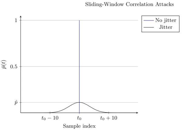
t0−10 t0 t0+ 10 ˆ
p
0.5 1
Sample index
¯
p
(
t
)
No jitter Jitter
Fig. 2: The probability of a leakage point position in the trace at sample points near the original leakage pointt0 as a function of the sample index, without and with jitter (sample drift normally distributed).
key byte value. Letρ(Hck, P) denote the Pearson correlation coefficient between these random variables.
Assume thatPorigis computed at sample indext0. When jitter is present, the leak that occurs at time t0 drifts due to hiding, meaning the observation of the leak may not be at sample t0, but might be within a range of sample indexes, either before or after t0. We denote the probability of the leak occurring in a specific sample index t by ¯p(t). Let ˆp denote maxtp¯(t). We assume that ˆp is achieved at the same sample index t0 that would likely contain the most of leakage points over the different traces, thus having the highest correlation ratio. This idea is illustrated in Figure 2, comparing the non-jittered case where there is certainty about the leakage sample index, and the jittered case with an example of normally distributed drift values.
For aligned power traces without jitter, ˆp= 1 because the leakage points all occur in the same sample number. However, for misaligned power traces ˆp6= 1, and the maximal correlation ratio between the observed power consumptionP and the correct key hypothetical power consumptionHck would be:
ρ(Hck, P) =ρ(Hck, Porig)·pˆ (1)
2.3 Sliding Window CPA attack on jittered CPU clocks
Algorithm 1 Sliding Window Correlation Power Analysis Attack (SW-CPA)
1: procedurePreprocessTrace(Trace, r) 2: fort∈T racedo
3: SummedTrace(t) =Pr/2
i=−r/2Trace(t+i) 4: returnSummedTrace
5: procedureAttack(r) 6: Acquire set of traces X
7: forT race∈X do
8: T race←P reprocessT race(T race, r). 9: Perform CPA on X.
“comb” function transformation. The original attack was performed with tradi-tional difference of means DPA (single bit model attack).
Our attack on jittered CPUs, which we call the Sliding Window Correla-tion Power Analysis attack (SW-CPA), is inspired by [CCD00]; we use a similar pre-processing idea but then we use a CPA attack (byte model attack). Further-more, unlike the example in [CCD00], we use only a single continuous integration window with a size of r(aggregating r consecutive samples instead of a sparse “comb” aggregation) — see Algorithm 1. The attack exploits the fact that al-though each trace’s leakage can happen at a different time due to jitter, with a high probability the leakages will occur within some radius r/2 of the original leakage sample point (without the counter-measure). If we then apply the CPA attack on the integrated traces, there would be a common trace sample index containing the leakage for many different traces. We chose to aggregate one con-tinuous window (rather than the comb-like integration of [CCD00]) as we cannot assume, without profiling, where the leakage would be, and we would like the drifted leakage points to be included within the integrated window.
2.4 Basic correlation analysis of sliding-window integration
To begin with, let us find the Pearson correlation coefficient of a key hypothesis with the pre-processed traces data-set, when no jitter is present and the traces are aligned. Without loss of generality assume that a leakage occurs at sample point 1. Letρ1 be the correlation coefficient between the leakage sampleP1 and the correct key hypothesisHck. Then, by definition we have:
ρ1≡ρ(Hck, P1) =
Cov(Hck, P1)
p
V ar(Hck)·V ar(P1) =
E(Hck·P1)−E(Hck)·E(P1)
p
V ar(Hck)·V ar(P1) (2)
In [MOP08] pp. 210-211, Mangard et al. analyzed the effect of the integration ofrindependent power samples,{P−r/2, . . . , P1, . . . , Pr/2}, containing exactly a single leakage sample. Their analysis shows that:
ρ(Hck, r/2
X
i=−r/2 Pi) =
ρ1 √
Equation (3) is clearly an upper bound on the correlation once jitter is intro-duced. Therefore, under the analyzed conditions there is a trade-off on setting the window sizer. On the one hand, when we increaser, we increase the likeli-hood that the leakage sample would be within our aggregation window because the drift value caused by jitter will be smaller thanr. Consequently, due to Equa-tion (1), we would like to increase the window size. On the other, EquaEqua-tion (3) seems to show that integration decreases the correlation by the square root of the window size, which would force the cryptanalyst to use many more traces to compensate.
3
A new analysis of multiple leakage samples integration
The conclusion from [MOP08] as seen in Equation (3) is that when using inte-gration, the samples’ noise is aggregated, and the correlation ratio drops. In this section we show that on the contrary, SW-CPA integration can be an effective technique which actually amplifies the correlation with and without jitter. We do this by using a different and very realistic model of the leakage observed in the power traces. In Section 4 we validate that our model assumptions indeed hold on traces collected from a real device with a jittered clock.
3.1 The correlation coefficient when integrating within a trace
The leakage model previously mentioned in Section 2.4 assumes only a single
leakage point within the integration window, and r−1 power samples inde-pendent of the encryption key (non leakage samples). However, there might be several leakage samples in a trace. Whenever the cryptanalyst observes more than one peak in the correlation coefficient in a CPA for the correct key byte, there is more than one leakage point. This may be caused by several reasons: multiple leakage sources may exist, such as data bus leakage, address bus leakage or different electronic components’ glitches which may all happen sequentially. Alternatively, a high sampling frequency of the measurement instrument may cause switching to spread over more than one sample. CPU architecture and software implementation may imply more phenomena creating such behavior. For example, Papagiannopoulos et al. [PV17] showed that the data might be loaded to several registers during the computation. As we shall see, in traces we collected (without jitter), we observed this phenomenon quite clearly: there were multiple leak points, relatively close to each other in time.
different sample points. Therefore, they have the same expectation and variance. Without loss of generality, assume thatP1 is a leakage sample point, so for all q(r) leakage samples Pi,Pj, (i6=j) we have:
E(Pi) =E(P1) V ar(Pi) =V ar(P1)
(4)
By definition for two leakage samples with same variance, using Pearson corre-lation coefficientρi,j between power samplesPi,Pj, we have:
Cov(Pi, Pj)≡qV ar(Pi)·V ar(Pj)·ρi,j =V ar(P1)·ρi,j (5)
For the other r−q(r) noise samples we can safely assume that they are inde-pendent of each other and of the leakage points. Therefore, for samples Pi, Pj where at least one is a noise samples, we get that Pi and Pj are uncorrelated, i.e.,Cov(Pi, Pj) = 0.
Next, we assume that while the expectations of the key-dependent and noise samples are different, they all have the same variance, since they are all subject to the same noise, i.e.,
V ar(Pi) =V ar(P1) for alli.
Hence, for all samples, regardless of the sample type (leakage or noise), we con-clude that for allPi ,Pj:
Cov(Pi, Pj) =
(
V ar(P1)·ρi,j i, j are leakage samples
0 Otherwise (6)
The noise samples are also independent of the correct key hypothesis (because they are not leakage points), so for such samplePi:
E(Hck·Pi) =E(Hck)·E(Pi) (7)
Now we return to the correlation coefficient. According to Equation (2), the correlation coefficient for rintegrated samples is:
ρ(Hck, r/2
X
i=−r/2 Pi) =
E(Hck·(P r/2
i=−r/2Pi))−E(Hck)·E(P r/2 i=−r/2Pi)
q
V ar(Hck)·V ar(Pr/2
i=−r/2Pi)
=
Pr/2
i=−r/2(E(Hck·Pi)−E(Hck)·E(Pi))
q
V ar(Hck))·V ar(P r/2 i=−r/2Pi)
We know there are exactly q(r) leakage samples. Separating the sums for key byte leakage and noise indexes, Equations (4) and (7) and the standard formula for the variance of a sum give:
ρ(Hck, r/2
X
i=−r/2
Pi) = q(r)·(E(Hck·P1))−E(Hck)·E(P1))
p
V ar(Hck)·
q Pr/2
By Equation (6) and plugging in the definition of ρ1 (non-jittered correlation without integration) from Equation (2) we can simplify the result to:
ρ(Hck, r/2
X
i=−r/2
Pi) = q(r)·(E(Hck·P1)−E(Hck)·E(P1))
p
V ar(Hck)·
q
r+P
i6=jρi,j·
p
V ar(P1) =⇒
ρ(Hck, r/2
X
i=−r/2 Pi) =
q(r)
q
r+P
i6=j,leakage samplesρi,j
·ρ1 (8)
Letγdenote the normalized sum of correlation coefficients of the leakage points:
γ≡ r+
P
i6=j,leakage samplesρi,j r
Then, we can rewrite Equation (8) as:
ρ(Hck, r/2
X
i=−r/2
Pi) = √q(r)
r·γ ·ρ1 (9)
If all the leakage points are uncorrelated samples thenρi,j = 0⇒γ = 1. Con-versely, in the worst case the leakage points are fully correlated withρi,j = 1⇒ γ=r. Becauseγis derived from the correlation matrix of random variables, it is positive semidefinite and in particular the sum of its items is non-negative, hence also γ ≥ 0. However,γ can be smaller than 1 causing a further amplification. Casting Equation (9) to also explicitly show the interesting cases we get
ρ(Hck, r/2
X
i=−r/2 Pi) =
q(r)
√
r ·ρ1 uncorrelated leakage samples q(r)
√
r·γ ·ρ1 partly correlated leakage samples q(r)
r ·ρ1 fully correlated samples
(10)
For simplicity, unless mentioned otherwise, in the derivations below we as-sume leakage samples are uncorrelated, hence:
γ= 1 (11)
As we shall see in Section 4.3, in the data we gatheredγ is quite close to 1 and much smaller thanr.
We can see that for the special case ofq(r) = 1 we get exactly Equation (3), i.e., the result of Mangard et al. [MOP08]. For the most special case, where r=q= 1 we obtain the standard CPA attack.
3.2 Correlation coefficient amplification:
LetPtbe the distribution of trace power values at sample indext. Let
ρcpa= max
be the achieved correlation coefficient of a regular CPA attack on the traces. Now, assume we conduct a SW-CPA with a window size ofr. Then let
ρr= max t ρ(Hck,
r/2
X
i=−r/2 Pt+i)
be the correlation achieved by SW-CPA with window sizer. Note thatρcpa≡ρ1. Bothρ1 andρrshould have similar jitter properties (or no jitter). We define the correlation coefficientamplificationto be:
Amplification=ρr/ρ1
The cryptanalyst’s goal is to maximize the amplification, to reveal as many secret key bytes as possible.
3.3 The correlation coefficient for specific r and q relationships
Equation (10) can be made concrete if we have an explicit connection between r andq. We first assume that each key byte has a maximal number of leakage points, qmax. Further, we assume that all qmax leakage points are temporally close: they are all located within a distance of r0 samples from each other. Therefore, whenr≥r0the window is called saturated andqstops growing with r. So we get:
q=
(
q(r) ifr < r0
qmax otherwise (saturation) (12)
With this assumption we analyze two important cases:
Constant number of leakage points In caser≥r0, our window contains all qmaxleakage points of the phenomenon. Increasing the window size any further does not change the value ofq. According to Equation (10), the correlation would be:
ρ(Hck, r/2
X
i=−r/2
Pi) = qmax√
r ·ρ1 (13)
Hence, whenrincreasesρdecreases, and forr > q2
maxthe correlation drops below ρ1 and eventually ρ−→ 0. Therefore, a cryptanalyst who seeks to maximize ρ, should select the value ofrto be the smallest possible value containing allqmax leakage points.
Constant ratio between r and q Another important case is when the in-tegration window is not saturated, and increasing r increases the number of leakage pointsqlinearly such thatq(r) =r/cfor some constantc. In this case:
ρ(Hck, r/2
X
i=−r/2 Pi) =
q(r) √
r ·ρ1= r/c √
r ·ρ1 =⇒
ρ(Hck, r/2
X
i=−r/2 Pi) =
√ r
c ·ρ1 (14)
The first implication of this equation is that when√r > cwe obtain thatρ > ρ1: in other words, without jitter, not only does integration not reduce the correla-tion coefficient, it can even amplify it. However, as we increaser, eventually the number of leakage points saturates, yielding a non constant ratio betweenrand q(r) and we fall back to Equation (13).
Therefore, according to Equations (13) and (14), we get that the relationship betweenρ, the correlation coefficient of the integrated non-jittered traces;r, the window size;q, the number of leakage points within the window; andc, the ratio betweenrandqis:
ρ(Hck, r/2
X
i=−r/2 Pi) =
√
r
c ·ρ1 r < r0,constant ratio betweenqandr
qmax√
r ·ρ1 r≥r0 (saturatedq)
(15)
Still assuming for simplicity thatγ= 1.
3.4 The correlation coefficient with an unstable clock
So far, our analysis of SW-CPA assumed a stable clock and aligned traces. When we use an unstable clock, the correlation coefficient is also affected by the prob-ability that the leakage signals happen in the window around the same point in time, as stated in Equation (1). We denote by ˆq(r) the number of leakage points in a window of sizerwhen jitter is present.
Combining ˆqleakage points and the case of uncorrelated samples in Equation (10) yields the general correlation coefficient for the jittered clock:
ρ(Hck, r/2
X
i=−r/2
Pi) =qˆ√(r)
r ·ρ1 (16)
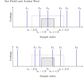
t0−J/2 t0 t0+J/2
t0−r/2 t0+r/2
L2 L3 L4 L5
L1 L6
Sample index
Leak
age
t0−J/2 t0 t0+J/2
t0−r/2 t0+r/2
L2 L3 L4 L5
L1 L6
Sample index
Leak
age
Fig. 3: Leakage vs. sample index for two specific traces. Blue lines are leakage points. The red dashed line is the possible drift region aroundt0. The gray area is the integration window aroundt0. The upper sub-figure is non-jittered while the lower sub-figure has jitter. The drift for the originalL3leakage point caused it to fall outside the window whileL4falls into the window.
Section 4.2). We seek to find the relation between ˆqandqfor different values of r. It is important to notice that the drift might change between different traces and different samples in the data-set.
For simplicity, we assume that the drift of a sample point is uniformly dis-tributed in time around the original non-jittered index, i.e.,Drif t∼U{−J
2 , J 2}. Because the drift is distributed uniformly and E(Drif t) = 0, the distance between the leakage points might increase as well as decrease, but it’s expectation is equal to the non-jittered case.
Figure 3 gives a schematic example for leakage samples, their drift over time, and how the number of leakage samples in the window is affected. We can see that although the original leakage point drifted, another leakage point was integrated in the window.
Therefore we get:
ˆ q(r) =
(q
max
r0+J ·r ifr < r0+J
qmax otherwise (saturation) (17)
The CPA correlation coefficient in the jittered case We first calculate ˆ
ρ1, the correlation coefficient for original CPA attack (r= 1) with jitterJ >1. The leakage signal originally always happens att0, but due to the jitter it may occur anywhere within the range [t0−J/2, t0+J/2].
According to Equation (17), the probability that a leakage point appears in sample indext0is:
ˆ
q(r= 1) = qmax r0+J
= r0 r0+J
·1
c (18)
due to the uniform leakage distribution.
Putting Equations (16) and (18) together gives the correlation ratio for the standard CPA (r= 1) against jittered traces:
ˆ ρ1=
ˆ q(r= 1)
√
r ·ρ1= r0 r0+J
·1
c ·ρ1 (19)
We can see that according to Equation (19), when jitter is present the standard CPA attack effectiveness is severely degraded — as we shall see in Section 5.2.
The SW-CPA Correlation coefficient for differentrvalues We now ana-lyze two important cases of r, caused by the different domains of ˆq in Equation (17), under the effect of a bounded jitter.
Constantq/r ratio: Whenr < r0+J from Equations (16) and (17), the corre-lation coefficient for SW-CPA is:
ρ(Hck, r/2
X
i=−r/2
Pi) = ˆq(r)·√1 r·ρ1=
qmax·r r0+J
·√1 r ·
r0+J r0
·c·ρˆ1 =⇒
ρ(Hck, r/2
X
i=−r/2 Pi) =
√
r·ρˆ1 (20)
Saturated qˆ values: The region around t0 when r ≥ r0 +J contains all the leakage points, meaning ˆq(r) =qmax. Combining Equations (16) and (19) gives forr≥r0+J:
ρ(Hck, r/2
X
i=−r/2
Pi) =qˆ√(r) r ·ρ1=
qmax √
r · r0+J
r0
·c·ρˆ1= r0+J
√
10 90 1000 1
2 4 8
Constantq/r Saturatedq
r
Amplification
Fig. 4: SW-CPA attack amplification of correlation coefficient (with jitter) vs. window size r (log scale) for J = 20, r0 = 70. The black line is the scenario for uncorrelated leakage samples (γ = 1). The blue line is for the worst case correlated leakage samples (γ=r). The dashed line atr= 90 separates the two regions of the amplification (constantq/r ratio and saturatedq). Amplification values above 1 indicate that ρ is amplified beyond the values for r = 1 (CPA attack on a jittered clock data-set).
Summarizing Equations (20) and (21), we get that the relationship between ρ, the correlation coefficient of the integrated jittered traces; ˆρ1, the correlation co-efficient without integration;r, the window size;q, the number of leakage points within the window;c, the ratio betweenrand q; replugging in the equation of γ from Equation (10); andJ, the maximal drift is:
ρ(Hck, r/2
X
i=−r/2 Pi) =
√
r
√
γ ·ρˆ1 r < r0+J,constant ratio betweenqandr
r0+J √
r·√γ ·ρˆ1 r≥r0+J (saturatedq)
(22)
The correlation coefficient with an unbounded jitter While our analysis assumed that the jitter is bounded (and in Section 4.2 we demonstrate this is a realistic assumption for our board), we argue that our analysis has merit in more general cases as well. Even if the jitter is unbounded we still expect to observe a randomly changing clock frequency according to some distribution. In such a case, we assume that using a reasonable clock spreading model, it should be possible to build a sample drift model in which with high probability the drift value would be in a specific range, thus making our analysis relevant. We leave the analysis of cases with unbounded jitter to future work.
4
Experiments and results
4.1 Setup and measurements
Our experimental setup centers around a Rabbit RCM4010 evaluation board. This device has a 59MHz processor with a 16-bit architecture [RCM10]. We programmed the board to implement an AES-128 algorithm using open-source code taken from [Con12]. This is a plain-vanilla software implementation of AES, without any side channel counter-measures or software optimizations (i.e., with-out using T-tables).
The Rabbit processor has a special feature called a spectrum-spreader — de-signed to reduce electromagnetic interference (EMI). Enabling the spreader in-troduces jitter into the CPU clock frequency. However, the documentation does not specify precisely how the spectrum-spreader works. Note that the Rabbit has two spreading modes, called Normal and Strong (in addition to no spread-ing mode), which can be selected by software. Our main experiments used the Normal mode, but additional experiments were conducted with Strong jitter and showed similar results.
We sampled the board power by a Lecroy WavePro 715Zi oscilloscope. When starting the execution of an encryption, we programmed the board to send a signal to the oscilloscope via one of its I/O pins which can be controlled by the software. This signal sets the trigger for the oscilloscope, which starts sampling at a rate of 500 million samples per second, for 500µs. This time period contains one round of the full AES encryption. Every encryption process is recorded to a new trace. The voltage of the processor was measured by a shunt resistor soldered to the processor voltage input. The input plaintexts for the program were changed every encryption round, while the key was kept constant during all traces. Two data-sets where captured; one consisted 5,000 traces without jitter and 5,600 traces with Normal jitter, using the same encryption key and plaintexts (for the first 5,000 jittered traces). The second and bigger data-set contains 10,000 traces of each spectrum-spreading mode: no spreading, Normal spreading and Strong spreading. These measurements were done with a different random key than the first data-set, but same plaintexts.
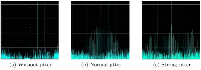
(a) Without jitter (b) Normal jitter (c) Strong jitter
Fig. 5: FFT magnitude vs. frequency of the power trace from RCM board, com-puted by the oscilloscope (a) without jitter, (b) with Normal jitter, (c) with Strong jitter, centered around 59MHz (original clock frequency) and axis be-tween 55-63 MHz
when the spectrum-spreader is turned on, the standard CPA attack is drastically degraded: without jitter the attack correctly discovers all 16 key bytes with as few as 2,500 traces, while with jitter CPA fails to identify more than two key bytes even with all 5,600 traces of the first data-set.
4.2 Jitter modeling
We first explored the jitter injected by the spectrum-spreader to validate the analysis of Section 3.4. This part was used for white-box validation of our leak-age model only and is not essential for the common adversary. When spectrum-spreading was enabled, frequency analysis revealed several new frequencies that appeared around the original 59MHz clock frequency, with about 0.15MHz dif-ference between them. Figure 5(a) shows the spectrum without jitter: notice the peaks at 59MHz and 60MHz (the former is the board clock frequency). Figure 5(b) shows the spectrum with Normal jitter: notice how the 59MHz peak is replaced by some 15-25 separate peaks while the irrelevant 60MHz peak is un-affected. Figure 5(c) shows the spectrum with Strong jitter: some 15 additional peaks appeared with higher and lower frequencies.
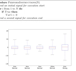
Algorithm 2 Drift assessment
1: procedurePerformInstructions(N) 2: Send an initial signal for execution start
3: forifrom 1 toN do
4: if T ruethen
5: V ar1←0
6: Send a second signal for execution end
Fig. 6: Drift in number of samples (D) vs. different execution duration (∆T) with the Normal and Strong spectrum-spreader. The red line is the median, the bottom and top of the boxes represent the first the third quartiles, and the whiskers range from the minimum to the maximum samples drift. Normal spreading is bounded by |D|= 10 samples and Strong spreading is bounded by |D|= 20 samples.
When Normal spreading was enabled∆T was not constant per execution length. We denote by D the difference, in number of samples, between the execution length with jitter and the constant execution length without jitter. For different execution lengths, we observed that the magnitude of the drift (|D|) wasbounded
by at most 10 samples (20ns) to each side, regardless of the execution length. Using the terminology of Section 3.4, the Rabbit Normal spectrum-spreader has a bound J = 20, |D| = 10. Similar experiments with the Strong spectrum-spreader showed that the drift is still bounded but withJ = 40,|D|= 20. The bounded drift in number of samples is illustrated by a box plot in Figure 6, for both Normal spreading and Strong spreading (box plots for additional Strong spreading execution lengths omitted).
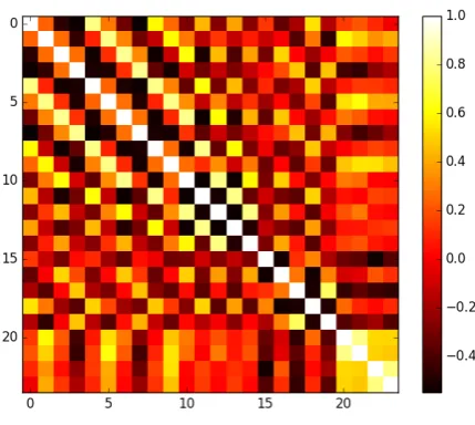
Fig. 7: Correlation matrix heat-map, for 25 leakage sample points for the best leakage window of key byte 7
cycle of jitter values can achieve the goal of EMI reduction, much more easily than generating true random, or cryptographic pseudo-random, clock jitter.
4.3 Validating leakage points’ power consumption correlation
101 102 1
1.5 2 2.5
25 50 0.5
r
ρ/
ˆ
ρ1
Byte 7 Byte 8 Byte 10
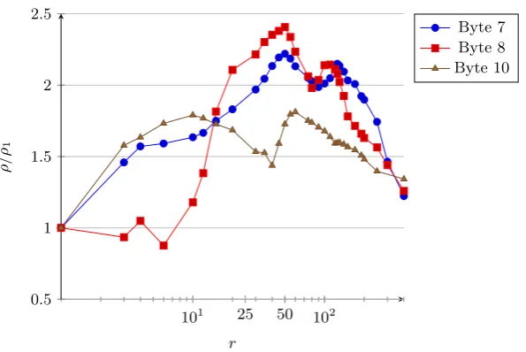
Fig. 8: Amplification of the correlation coefficient vs. window sizer (log scale), for three correct key bytes, with the jittered clock data-set of 5,600 traces. Am-plification values above 1 indicate thatρis amplified beyond the values forr= 1.
5
Evaluating the SW-CPA attack
5.1 Amplification for different aggregation window sizes
To calibrate the best window size r we examined leaks from the different key bytes in our encryption process. Figure 8 shows the amplification of the corre-lation coefficient for different window sizes and different correct key bytes when the CPU clock is jittered. Note that these key bytes are not identified correctly by CPA without pre-processing due to jitter. For simplicity, we do not show all key bytes.
The amplification graphs for all key bytes have major similarities. First, they all have an amplification higher than 1 for some window sizer, which helps the correct key byte detection and supports SW-CPA as an effective solution for the unstable clock counter-measure. In addition, they all suffer degradation whenr grows beyond a certain point andqreaches saturation. Finally, we see that the amplification does not increase monotonically toward a single peak — unlike the prediction in Figure 4. We explore this issue below.
option is that the leakage samples are correlated in a way that γ is relatively small for this small window of leakage samples.
5.2 Selecting a window size r for all key bytes
Next, we determine the single, best,rvalue of all key bytes for our device. Figure 9 shows the overall SW-CPA success rate for differentrvalues together with the results for standard CPA on non-jittered traces (as an ideal) and CPA on the jittered traces (as a worst-case).
The metric we used to recognize a correct key byte detection counted a correct key byte when the true key byte was within the highest five correlation possibilities, i.e., the key byte recovery is of the 5th order as stated in [SMY09]. This metric was chosen because a cryptanalyst can iterate (brute force) over the remaining 516≈237 options.
We’ve experimentally seen in Figure 8 that the ρ amplification graphs for separate key bytes had the highest peaks between 25 < r <75. We chose the overall value ofr= 75 experimentally, without profiling information, simply by running the attacks.
Figure 9 shows clearly that SW-CPA is very effective attack and defeats the clock jitter counter-measure well: for values of 10≤r≤75 it finds 12-14 correct key bytes with ≈ 4500 traces — only twice as many traces as needed for an equivalent success rate on non-jittered traces. Further, we see that our attack is not very sensitive to the value ofr: values between 10≤r≤75 are roughly equally successful. The figure shows that a larger window such asr= 150 gives a poor amount of true key byte detections. Window sizes below r = 10 have inferior performance (graphs omitted).
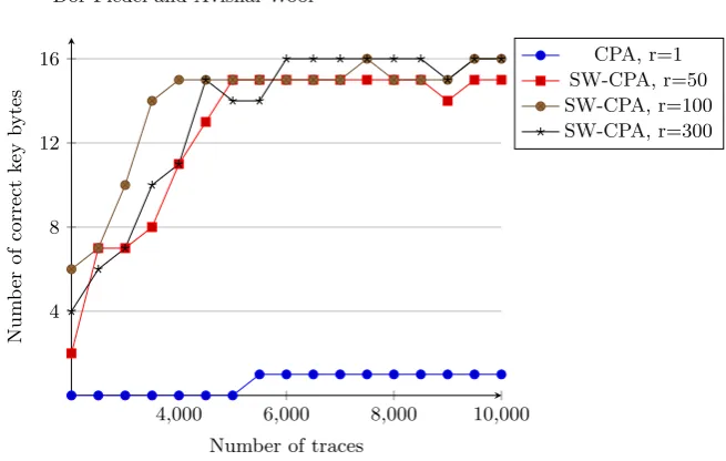
Figure 10 shows similar results for a larger data-set (10,000 traces) with a different key and Strong spectrum-spreading. The figure shows that SW-CPA is very successful against Strong jitter as well: it correctly finds all key bytes, with about 6,000 traces, for many window sizes, whereas regular CPA cannot find two correct key bytes even with all 10,000 traces. In addition, the higher drift with Strong jitter causes SW-CPA with large window size such as r = 300 to be effective and find 15-16 key bytes, whereas with Normal spreading (Figure 9) r= 150 was already too high and performance was degraded in comparison to r= 75.
2,000 3,000 4,000 5,000 4
8 12 16
Number of traces
Num
b
er
of
correct
k
ey
b
ytes
CPA, no jitter SW-CPA, r=75, jitter SW-CPA, r=10, jitter SW-CPA, r=150, jitter
CPA (r=1), jitter
Fig. 9: Number of correct key bytes vs. number of traces, for different values of the integration window size rand Normal Jitter
5.3 Comparing SW-CPA with other known methods
We compare the SW-CPA method (with the best integration window size) to previously suggested methods: trace selection pre-processing [HHO15], align-ment pre-processing [TH12,vWWB11,BHvW12], and frequency analysis attacks [SDB+10]. Figure 11 summarizes the results.
Applying the methods suggested in [HHO15,TH12] of pre-processing accord-ing to simple trace properties was inapplicable to our data-set. These attacks were originally performed on hardware encryption implementations and assume that the power consumption measurements have clearly visible patterns of the AES rounds. Our data with a software implementation on the Rabbit board exhibited no such patterns. We tried searching for the patterns with different sampling frequencies and different number of samples but the expected 10 spikes marking the 10 AES rounds did not manifest themselves in the power traces. A possibility why we did not observe the patters is that the Rabbit board we used is not idle between the encryption cycles or when waiting for input. Because the attacks rely on the visible encryption rounds, the device cannot be attacked by these methods.
4,000 6,000 8,000 10,000 4
8 12 16
Number of traces
Num
b
er
of
correct
k
ey
b
ytes
CPA, r=1 SW-CPA, r=50 SW-CPA, r=100 SW-CPA, r=300
Fig. 10: Number of correct key bytes vs. number of traces, for different values of the integration window sizerand large data-set with Strong spectrum-spreading.
Therefore, the methods of pre-processing according to simple trace properties and PCA [HHO15,TH12,BHvW12] detected zero key bytes correctly, and were not inserted to the comparison in Figure 11.
The method of elastic alignment [vWWB11] did not give us a high percent-age of correct key byte detection either (as was also observed by others who tested it with non-simulated data-sets [OP11,GPPT15]). The original article [vWWB11] offers a way to overcome the computational complexity of DTW by using FDTW, which is an approximation for DTW. We first implemented and tested FDTW with poor results. After FDTW failed, we applied the full DTW (with just the relevant alignment margin because of our bounded jitter) which slightly improved the results. Figure 11 shows the results of the improved DTW implementation.
The method of Correlation Power Frequency Analysis (CPFA) [SDB+10] was previously offered as a method for handling the start-point misalignment, because the magnitude in the frequency domain is not affected by time domain shifting. The results of this method were poor as well. We tried to optimize this attack as well, by targeting leakage areas, but results stayed the same.
Comparison to SW-DPA was more challenging. Clavier et al. [CCD00] did not suggest a way to determine their algorithm’s parameters, hence we do not see how to compare their general approach to our specific instantiation. However, their SW-DPA with 1-bit difference of means using our integration parameters gave poor results and was omitted from the comparison figure.
2,000 3,000 4,000 5,000 4
8 12 16
Number of traces
Num
b
er
of
correct
k
ey
b
ytes
CPA, no jitter SW-CPA (r= 75), jitter
CPA, jitter DTW, jitter CPFA, jitter
Fig. 11: Number of correct bytes vs. number of traces, for different implemented attacks. Attacks with 0 key bytes successfully detected were omitted. We also show the success rate of the standard CPA attack on non-jittered data (as an ideal).
Figure 11 clearly shows that SW-CPA yields far better true key byte detection results than the other possible solutions we tried. All the other solutions did not have more than two correct key bytes detections on our data-set with 5,600 traces. However, note that the unstable clock still degregates the attack: even our best SW-CPA requires approximately twice the number of traces to achieve an equivalent level of success in comparison to standard CPA against a non-jittered device.
6
Conclusions
References
BCO04. Eric Brier, Christophe Clavier, and Francis Olivier. Correlation power analysis with a leakage model. InCryptographic Hardware and Embedded Systems (CHES), pages 16–29. Springer, 2004.
BHvW12. Lejla Batina, Jip Hogenboom, and Jasper GJ van Woudenberg. Getting more from PCA: First results of using principal component analysis for ex-tensive power analysis. InCT-RSA, volume 7178, pages 383–397. Springer, 2012.
CCD00. Christophe Clavier, Jean-S´ebastien Coron, and Nora Dabbous. Differential power analysis in the presence of hardware countermeasures. In Crypto-graphic Hardware and Embedded Systems (CHES), pages 13–48. Springer, 2000.
CDP17. Eleonora Cagli, C´ecile Dumas, and Emmanuel Prouff. Convolutional neural networks with data augmentation against jitter-based countermeasures. In
International Conference on Cryptographic Hardware and Embedded Sys-tems (CHES), pages 45–68. Springer, 2017.
Con12. Brad Conte. Basic implementations of standard cryptography al-gorithms, like AES and SHA-1, 2012. https://github.com/B-Con/ crypto-algorithms.
CRR02. Suresh Chari, Josyula R Rao, and Pankaj Rohatgi. Template attacks. In
International Workshop on Cryptographic Hardware and Embedded Systems (CHES), pages 13–28. Springer, 2002.
FH08. Julie Ferrigno and M Hlav´aˇc. When AES blinks: introducing optical side channel.IET Information Security, 2(3):94–98, 2008.
GM11. Tim G¨uneysu and Amir Moradi. Generic side-channel countermeasures for reconfigurable devices.Cryptographic Hardware and Embedded Systems (CHES), pages 33–48, 2011.
GPPT15. Daniel Genkin, Lev Pachmanov, Itamar Pipman, and Eran Tromer. Steal-ing keys from PCs usSteal-ing a radio: Cheap electromagnetic attacks on win-dowed exponentiation. InInternational Workshop on Cryptographic Hard-ware and Embedded Systems (CHES), pages 207–228. Springer, 2015. HHO15. Philip Hodgers, Neil Hanley, and Maire O’Neill. Pre-processing power
traces to defeat random clocking countermeasures. InInternational Sym-posium on Circuits and Systems (ISCAS), pages 85–88. IEEE, 2015. HNI+06. Naofumi Homma, Sei Nagashima, Yuichi Imai, Takafumi Aoki, and Akashi
Satoh. High-resolution side-channel attack using phase-based waveform matching. In Cryptographic Hardware and Embedded Systems (CHES), pages 187–200. Springer, 2006.
KA98. Markus G Kuhn and Ross J Anderson. Soft tempest: Hidden data trans-mission using electromagnetic emanations. InInformation hiding, volume 1525, pages 124–142. Springer, 1998.
KJJ99. Paul Kocher, Joshua Jaffe, and Benjamin Jun. Differential power analysis. InAdvances in cryptology (CRYPTO), pages 789–789. Springer, 1999. Koc96. Paul C Kocher. Timing attacks on implementations of Diffie-Hellman, RSA,
DSS, and other systems. InAnnual International Cryptology Conference, pages 104–113. Springer, 1996.
MvWB11. Ruben A Muijrers, Jasper GJ van Woudenberg, and Lejla Batina. RAM: Rapid alignment method. In International Conference on Smart Card Research and Advanced Applications (CARDIS), pages 266–282. Springer, 2011.
OC15. Colin O’Flynn and Zhizhang Chen. Synchronous sampling and clock re-covery of internal oscillators for side channel analysis and fault injection.
Journal of Cryptographic Engineering, 5(1):53–69, 2015.
OP11. David Oswald and Christof Paar. Breaking MILFARE DESFIRE MF3ICD40: Power analysis and templates in the real world. In Cryp-tographic Hardware and Embedded Systems (CHES), pages 207–222. Springer, 2011.
OP12. David Oswald and Christof Paar. Improving side-channel analysis with optimal linear transforms. In International Conference on Smart Card Research and Advanced Applications, pages 219–233. Springer, 2012. PV17. Kostas Papagiannopoulos and Nikita Veshchikov. Mind the gap: Towards
secure 1st-order masking in software. InIACR Cryptology ePrint Archive, page 345, 2017.
RCM10. Digi International Inc. RabbitCore RCM4000 user manual, 2010. http: //ftp1.digi.com/support/documentation/019-0157_J.pdf.
SDB+10. Oliver Schimmel, Paul Duplys, Eberhard Boehl, Jan Hayek, R Bosch, and W Rosenstiel. Correlation power analysis in frequency domain. In
COSADE First International Workshop on Constructive Side Channel Analysis and Secure Design, 2010.
SMY09. Fran¸cois-Xavier Standaert, Tal Malkin, and Moti Yung. A unified frame-work for the analysis of side-channel key recovery attacks. InEurocrypt, volume 5479, pages 443–461. Springer, 2009.
ST04. Adi Shamir and Eran Tromer. Acoustic cryptanalysis. 2004. presentation available fromhttp://www.wisdom.weizmann.ac.il/~tromer.
TH12. Qizhi Tian and Sorin A Huss. On the attack of misaligned traces by power analysis methods. In Computer Engineering & Systems (ICCES), 2012 Seventh International Conference on, pages 28–34. IEEE, 2012.