Multirate Simulations of String Vibrations Including Nonlinear Fret String Interactions Using the Functional Transformation Method

Multirate Simulations of String Vibrations Including

Nonlinear Fret-String Interactions Using

the Functional Transformation Method

L. Trautmann

Multimedia Communications and Signal Processing, University of Erlangen-Nuremberg, Cauerstrasse 7, 91058 Erlangen, Germany Email:[email protected]

Laboratory of Acoustics and Audio Signal Processing, Helsinki University of Technology, P.O. Box 3000, 02015 Espoo, Finland Email:[email protected]

R. Rabenstein

Multimedia Communications and Signal Processing, University of Erlangen-Nuremberg, Cauerstrasse 7, 91058 Erlangen, Germany Email:[email protected]

Received 30 June 2003; Revised 14 November 2003

The functional transformation method (FTM) is a well-established mathematical method for accurate simulations of multidimen-sional physical systems from various fields of science, including optics, heat and mass transfer, electrical engineering, and acoustics. This paper applies the FTM to real-time simulations of transversal vibrating strings. First, a physical model of a transversal vibrat-ing lossy and dispersive strvibrat-ing is derived. Afterwards, this model is solved with the FTM for two cases: the ideally linearly vibratvibrat-ing string and the string interacting nonlinearly with the frets. It is shown that accurate and stable simulations can be achieved with the discretization of the continuous solution at audio rate. Both simulations can also be performed with a multirate approach with only minor degradations of the simulation accuracy but with preservation of stability. This saves almost 80% of the compu-tational cost for the simulation of a six-string guitar and therefore it is in the range of the compucompu-tational cost for digital waveguide simulations.

Keywords and phrases:multidimensional system, vibrating string, partial differential equation, functional transformation, non-linear, multirate approach.

1. INTRODUCTION

Digital sound synthesis methods can mainly be categorized into classical direct synthesis methods and physics-based methods [1]. The first category includes all kinds of sound processing algorithms like wavetable, granular and subtrac-tive synthesis, as well as abstract mathematical models, like additive or frequency modulation synthesis. What is com-mon to all these methods is that they are based on the sound to be (re)produced.

The physics-based methods, also called physical model-ing methods, start at the physics of the sound production mechanism rather than at the resulting sound. This approach has several advantages over the sound-based methods.

(i) The resulting sound and especially transitions be-tween successive notes always sound acoustically realistic as far as the underlying model is sufficiently accurate.

(ii) Sound variations of acoustical instruments due to

dif-ferent playing techniques or different instruments within one instrument family are described in the physics-based meth-ods with only a few parameters. These parameters can be ad-justed in advance to simulate a distinct acoustical instrument or they can be controlled by the musician to morph between real world instruments to obtain more degrees of freedom in the expressiveness and variability.

The second item makes physical modeling methods quite useful for multimedia applications where only a very limited bandwidth is available for the transmission of music as, for example, in mobile phones. In these applications, the physi-cal model has to be transferred only once and afterwards it is sufficient to transfer only the musical score while keeping the variability of the resulting sound.

vibrating object results in time, continuous-space models. These models are called initial-boundary-value problems and they contain a partial differential equa-tion (PDE) and some initial and boundary condiequa-tions. The discretization approaches to the continuous models and the digital realizations are different for the single physical mod-eling methods.

One of the first physical modeling algorithm for the sim-ulation of musical instruments was made by Hiller and Ruiz 1971 in [2] with the finite difference method. It directly dis-cretizes the temporal and spatial differential operators of the PDE to finite difference terms. On the one hand, this ap-proach is computationally very demanding; since temporal and spatial sampling intervals have to be chosen small for accurate simulations. Furthermore, stability problems occur especially in dispersive vibrational objects if the relationship between temporal and spatial sampling intervals is not cho-sen properly [3]. On the other hand, the finite difference method is quite suitable for studies in which the vibration has to be evaluated in a dense spatial grid. Therefore, the finite difference method has mainly been used for academic stud-ies rather than for real-time applications (see, e.g., [4,5]). However, the finite difference method has recently become more popular also for real-time applications in conjunction with other physical modeling methods [6,7].

A mathematically similar discretization approach is used in mass-spring models that are closely related to the finite element method. In this approach, the vibrating structure is reduced to a finite number of mass points that are inter-connected by springs and dampers. One of the first systems for the simulation of musical instruments was the CORDIS system which could be realized in real time on a specialized processor [8]. The finite difference method, as well as the mass-spring models, can be viewed as direct discretization approaches of the initial-boundary-value problems. Despite the stability problems, they are very easy to set up, but they are computationally demanding.

In modal synthesis, first introduced in [9], the PDE is spatially discretized at non necessarily equidistant spatial points, similar to the mass-spring models. The interconnec-tions between these discretized spatial points reflect the phys-ical behavior of the structure. This discretization reduces the degrees of freedom for the vibration to the number of spatial points which is directly transferred to the same number of temporal modes the structure can vibrate in. The reduction does not only allow the calculation of the modes of simple structures, but it can also handle vibrational measurements of more complicated structures at a finite number of spatial points [10]. A commercial product of the modal synthesis, Modalys, is described, for example, in [11]. For a review of modal synthesis and a comparison to the functional trans-formation method (FTM), see also [12].

The commercially and academically most popular phys-ical modeling method of the last two decades was the digital waveguide method (DWG) because of its computational ef-ficiency. It was first introduced in [13] as a physically inter-preted extension of the Karplus-Strong algorithm [14]. Ex-tensions of the DWG are described, for example, in [15,16,

17,18]. The DWG first simplifies the PDE to the wave equa-tion which has an analytical soluequa-tion in the form of a for-ward and backfor-ward traveling wave, called d’Alembert solu-tion. It can be realized computationally very efficient with delay lines. The sound effects like damping or dispersion oc-curring in the vibrating structure are included in the DWG by low-order digital filters concentrated in one point of the de-lay line. This procedure ensures the computational efficiency, but the implementation looses the direct connection to the physical parameters of the vibrating structure.

The focus of this article is the FTM. It was first intro-duced in [19] for the heat-flow equation and first used for digital sound synthesis in [20]. Extensions to the basic model of a vibrating string and comparisons between the FTM and the above mentioned physical modeling methods are given, for example, in [12]. In the FTM, the initial-boundary-value problem is first solved analytically by appropriate functional transformations before it is discretized for computer simula-tions. This ensures a high simulation accuracy as well as an inherent stability. One of the drawbacks of the FTM is so far its computational load, which is about five times higher than the load of the DWG [21].

This article extends the FTM by applying a multirate ap-proach to the discrete realization of the FTM, such that the computational complexity is significantly reduced. The ex-tension is shown for the linearly vibrating string as well as for the nonlinear limitation of the string vibration by a fret-string interaction occurring in slapbass synthesis.

The article is organized as follows.Section 2derives the physical model of a transversal vibrating, dispersive, and lossy string in terms of a scalar PDE and initial and boundary conditions. Furthermore, a model for a nonlinear fret-string interaction is given. These models are solved in Section 3 with the FTM in continuous time and continuous space. Section 4discretizes these solutions at audio rate and derives an algorithm to guarantee stability even for the nonlinear discrete system. A multirate approach is used in Section 5 for the simulation of the continuous solution to save com-putational cost. It is shown that this multirate approach also works for nonlinear systems. Section 6compares the audio rate and the multirate solutions with respect to the simula-tion accuracy and the computasimula-tional complexity.

2. PHYSICAL MODELS

In this Section, a transversal vibrating, dispersive, and lossy string is analyzed using the basic laws of physics. From this analysis, a scalar PDE is derived in Section 2.1.Section 2.2 defines the initial states of the vibration, as well as the fixings of the string at the nut and the bridge end, in terms of ini-tial and boundary conditions, respectively. InSection 2.3, the linear model is extended with a deflection-dependent force simulating the nonlinear interaction between the string and the frets, well known as slap synthesis [22].

neither the cross section area nor the tension on the string so that the string itself behaves linearly.

2.1. Linear partial differential equation derived by basic laws of physics

The string under examination is characterized by its ma-terial and geometrical parameters. The mama-terial parameters are given by the mass densityρ, the Young’s modulusE, the laminar air flow damping coefficientd1, and the viscoelastic

damping coefficientd3. The geometrical parameters consist

of the lengthl, the cross section areaAand the moment of inertiaI. Furthermore, a tensionTsis applied to the string in

axial direction. Considering only a string segment between the spatial positionsxsandxs+∆x, the forces on this string

segment can be analyzed in detail. They consist of the restor-ing force fT caused by the tensionTs, the bending force fB

caused by the stiffness of the string, the laminar air flow force

fd1, the viscoelastic damping forcefd3(modeled here without

memory), and the external excitation force fe. They result at

xsin

notes spatial derivative and dot denotes temporal derivative. Note that in (1a) and in (1d) it is assumed that the amplitude of the string vibration is small so that the sine function can be approximated by its argument. Similar equations can be found for the forces at the other end of the string segment at

xs+∆x.

All these forces are combined by the equation of motion to

coupled equations are obtained, that are valid not only at the string segmentxs≤x≤xs+∆xbut also at the whole string An extended version of the derivation of (3) can be found in [12]. The four coupled equations (3) can be simplified to one scalar PDE with only one output variable. All the dependent variables in (3a) can be written in terms of the

string deflection y(x,t) by replacingv(x,t) with ˙y(x,t) and

ϕ(x,t)=y(x,t) from (3d) and with (3b) and (3c). Then (3) can be written in a general notation of scalar PDEs

Dy(x,t)+ Ly(x,t)+ Wy(x,t) poral derivatives, the operator L{}has only spatial deriva-tives, and the operator W{}consists of mixed temporal and spatial derivatives. The PDE is valid only on the string be-tweenx = 0 andx =land for all positive times. Equation (4) forms a continuous-time, continuous-space PDE. For a unique solution, initial and boundary conditions must be given as specified in the next section.

2.2. Initial and boundary conditions

Initial conditions define the initial state of the string at time

t=0. This definition is written in the general operator nota-tion with

Since the scalar PDE (4) is of second order with respect to time, only two initial conditions are needed. They are chosen arbitrarily by the initial deflection and the initial velocity of the string as seen in (5). For musical applications, it is a rea-sonable assumption that the initial states of the strings vanish at timet=0 as given in (5). Note that this does not prevent the interaction between successively played notes since the time is not set to zero for each note. Thus, this kind of initial condition is only used for, for example, the beginning of a piece of music.

In addition to the initial conditions, also the fixings of the string at both ends must be defined in terms of bound-ary conditions. In most stringed instruments, the strings are nearly fixed at the nut end (x=x0=0) and transfer energy

at the other end (x=x1 =l) via the bridge to the resonant

PDE IC, BC

L{·} ODE BC

T{·} Algebraic equation

Discrete MD TFM Discrete

1−D TFM Discrete

solution

MD TFM Reordering

Discretization

T−1_{·}

z−1_{·}

Figure1: Procedure of the FTM solving initial boundary value problems defined in form of PDEs, IC, and BC.

into the system via the boundary, resulting in homogeneous boundary conditions.

The PDE (4), in conjunction with the initial (5) and boundary conditions (6), forms the linear continuous-time continuous-space initial-boundary-value problem to be solved and simulated.

2.3. Nonlinear extension to the linear model for slap synthesis

Nonlinearities are an important part in the sound produc-tion mechanisms of musical instruments [23]. One example is the nonlinear interaction of the string with the frets, well known as slap synthesis. This effect was modeled first for the DWG in [22] as a nonlinear amplitude limitation. For the FTM, the effect was already applied to vibrating strings in [24].

A simplified model for this interaction interprets the fret as a spring with a high stiffness coefficientSfretacting at one

positionxf as a forceffon the string at time instances where

the string is in contact with the fret. Since this force depends on the string deflection, it is nonlinear, defined with

ff

xf,t,y,yf

=

  Sfret

yxf,t

−yf

xf,t

, foryxf,t

−yf

xf,t

>0,

0, foryxf,t

−yf

xf,t

≤0.

(7)

The deflection of the fret from the string rest position is de-noted withyf. The PDE (4) becomes nonlinear by adding the

slap force ffto the excitation function fe1(x,t). Thus, a linear

and a nonlinear system for the simulation of the vibrating string is derived. Both systems are solved in the next sections with the FTM.

3. CONTINUOUS SOLUTIONS USING THE FTM

To obtain a model that can be implemented in the computer, the continuous initial-boundary-value problem has to be discretized. Instead of using a direct discretization approach as described inSection 1, the continuous analytical solution is derived first, which is discretized subsequently. This proce-dure is well known from the simulation of one-dimensional systems like electrical networks. It has several advantages in-cluding simulation accuracy and guaranteed stability.

The outline of the FTM is given in Figure 1. First, the PDE with initial conditions (IC) and boundary conditions

(BC) is Laplace transformed (L{·}) with respect to time to derive a boundary-value problem (ODE, BC). Then a so-called Sturm-Liouville transformation (T{·}) is used for the spatial variable to obtain an algebraic equation. Solving for the output variable results in a multidimensional (MD) transfer function model (TFM). It is discretized and by ap-plying the inverse Sturm-Liouville transformation T−1_{·}

and the inversez-transformationz−1_{{·}it results in the}

dis-cretized solution in the time and space domain.

The impulse-invariant transformation is used for the dis-cretization shown inFigure 1. It is equivalent to the calcu-lation of the continuous solution by inverse transformation into the continuous time and space domain with subsequent sampling. The calculation of the continuous solution is pre-sented in Sections3.1to3.5, the discretization is shown in Sections4and5.

For the nonlinear system, the transformations cannot ob-viously result in a TFM. Therefore, the procedure has to be modified slightly, resulting in an MD implicit equation, de-scribed inSection 3.6.

3.1. Laplace transformation

As known from linear electrical network theory, the Laplace transformation removes the temporal derivatives in linear and time-invariant (LTI) systems and includes, due to the differentiation theorem, the initial conditions as additive terms (see, e.g., [25]). Since first- and second-order time derivatives occur in (4) and the initial conditions (5) are ho-mogeneous, the application of the Laplace transformation to the initial boundary value problem derived inSection 2 re-sults in

dD(s)Y(x,s) + L

Y(x,s)+wD(s)WL

Y(x,s) =Fe1(x,s), x∈[0,l],

(8a)

f_bT_iY(x,s)=0, i∈0, 1. (8b) The Laplace transformed functions are written with capital letters and the complex temporal frequency variable is de-noted bys=σ+jω. It can be seen in (8a) that the temporal derivatives of (4a) are replaced with scalar multiplication of the functions

dD(s)=ρAs2+d1s, wD(s)= −d3s. (8c)

3.2. Sturm-Liouville transformation

The transformation of the spatial variable should have the same properties as the Laplace transformation has for the time variable. It should remove the spatial derivatives and it should include the boundary conditions as additive terms. Unfortunately, there is no unique transformation available for this task due to the finite spatial definition range in con-trast to the infinite time axis. That calls for a determination of the spatial transformation at hand, depending on the spa-tial differential operator and the boundary conditions. Since it leads to an eigenvalue problem first solved for simplified problems by Sturm and Liouville between 1836 and 1838, this transformation is called a Sturm-Liouville transforma-tion (SLT) [26]. Mathematical details of the SLT applied to scalar PDEs can be found in [12].

The SLT is defined by

TY(x,s)=_Y¯_(µ,s)=

_l

0K(µ,x)Y(x,s)dx. (9)

Note that there is a finite integration range in (9) in contrast to the Laplace transformation. The transformation kernels

K(µ,x) of the SLT are obtained as the set of eigenfunctions of the spatial operator LW=L + WLwith respect to the

bound-ary conditions (8b). The corresponding eigenvalues are de-noted byβ4

µ(s) where βµ(s) is the discrete spatial frequency variable (see, e.g., [12] for details).

For the boundary-value problem defined in (8) with the operators given in (4b), the transformation kernels and the discrete spatial frequency variables result in

K(µ,x)=sin

Thus, the SLT can be interpreted as an extended Fourier se-ries decomposition.

3.3. Multidimensional transfer function model

Applying the SLT (9) to the boundary-value problem (8) and solving for the transformed output variable ¯Y(µ,s) results in the MD TFM

Hence, the transformed input forces ¯F(µ,s) are related via the MD transfer function given in (11) to the transformed output variable ¯Y(µ,s). The denominator of the MD TFM depends quadratically on the temporal frequency variables

and to the power of four on the spatial frequency variableβµ. This is based on the second-order temporal and fourth-order spatial derivatives occurring in the scalar PDE (4). Thus, the transfer function is a two-pole system with respect to time for each discrete spatial eigenvalueβµ.

3.4. Inverse transformations

As explained at the beginning of Section 3, the continuous solution in the time and space domain is now calculated by using inverse transformations.

Inverse SLT

The inverse SLT is defined by an infinite sum over all discrete eigenvaluesβµwith

The inverse transformation kernel K(µ,x) and the inverse spatial frequency variableβµare the same eigenfunctions and eigenvalues as for the forward transformation due to the self-adjointness of the spatial operators L and WL(see [12] for

de-tails). Thus, the inverse SLT can be evaluated at each spatial position by evaluating the infinite sum. Since only quadratic terms ofµoccur in the denominator, it is sufficient to sum over positive values ofµand double the result to account for the negative values. The norm factor results in that case in

Nµ=l/4.

Inverse Laplace transformation

It can be seen from (11) and (8c), (10b) that the transfer functions consist of two-pole systems with conjugate com-plex pole pairs for each discrete spatial eigenvalueβµ. There-fore the inverse Laplace transformation results for each spa-tial frequency variable in a damped sinusoidal term, called mode.

3.5. Continuous solution

After applying the inverse transformations to the MD TFM, the continuous solution results in

y(x,t)= 4

tion is only valid for positive time instances;∗means tem-poral convolution. ¯fe(x,t) is the spatially transformed

exci-tation force, derived by inserting fe1 into (9). The angular

frequenciesωµ, as well as their corresponding damping co-efficientsσµ, can be calculated from the poles of the transfer function model (11). They directly depend on the physical parameters of the string and can be expressed by

ωµ=

3.6. Implicit equation for slap synthesis

The PDE (4) becomes nonlinear by adding the solution-dependent slap force ff(xf,t,y,yf) in (7) to the right-hand

side of the linear PDE. Obviously, the application of the Laplace transformation and the SLT to the nonlinear initial-boundary-value problem cannot lead to an MD TFM, since a TFM always requires linearity. However, assuming that the nonlinearity can be represented as a finite power series and that the nonlinearity does not contain spatial derivatives, both transformations can be applied to the system [12]. With (7), both premises are given such that the slap force can also be transformed into the frequency domains. The Y(x,s )-dependency of ¯Ff can be expressed with (12) in terms of

¯

Y(ν,s) to be consistently in the spatial frequency domain. Then an MD implicit equation is derived in the temporal and spatial frequency domain

¯

Y(µ,s)= 1

dD(s) +β4µ(s)

_¯

Fe(µ,s) + ¯Ff

µ,s, ¯Y(ν,s). (15) Note that the different argumentνin the output dependence of ¯Ff(µ,s, ¯Y(ν,s)) denotes an interaction between all modes

caused by the nonlinear slap force. Details can be found in [12].

Since the transfer functions in (11) and (15) are the same, also the spatial transformation kernels and frequency vari-ables stay the same as in the linear case. Thus, also the tem-poral poles of (15) are the same as in the MD TFM (11) and the continuous solution results in the implicit equation

y(x,t)= 4

ρAl

∞

µ=1

1

ωµe

σµt_sinω µt

∗_f¯_{e(x,t) + ¯ffµ,t, ¯y(ν,t)}

×K(µ,x)δ−1(t),

(16)

withωµandσµgiven in (14). It is shown in the next sections that this implicit equation is turned into explicit ones by ap-plying different discretization schemes.

4. DISCRETIZATION AT AUDIO RATE

This section describes the discretization of the continuous solutions for the linear and the nonlinear cases. It is per-formed at audio rate, for example with sampling frequency

fs=1/T=44.1 kHz, whereTdenotes the sampling interval.

The discrete realization is shown as it can be implemented in the computer. For the nonlinear slap synthesis, some ex-tensions of the discrete realization are required and, further-more, the stability of the entire system must be controlled.

4.1. Discretization of the linear MD model

The discrete realization of the MD TFM (11) consists of a three-step procedure performed below:

(1) discretization with respect to time, (2) discretization with respect to space, (3) inverse transformations.

Discretization with respect to time

Discretizing the time variable witht=kT,k∈Nand assum-ing an impulse-invariant system, an s-to-z mapping is ap-plied to the MD TFM (11) withz=e−sT_{. This procedure} di-rectly leads to an MD TFM with the discrete-time frequency variablez:

¯

Yd_(µ,z)= T

1/ρAωµ

zeσµT_sinω µT

z2_−2zeσµT_cosωµT+e2σµT ¯

Fd

e(µ,z). (17)

Superscript d denotes discretized variables. The angular fre-quency variables and the damping coefficients are given in (14). Pole-zero diagrams of the continuous and the discrete system are shown in [27].

Discretization with respect to space

For the spatial frequency domain, there is no need for cretization, since the spatial frequency variable is already dis-crete. However, a discretization has to be applied to the spa-tial variablex. This spatial discretization consists of simply evaluating the analytical solution (13) at a limited number of arbitrary spatial positionsxa on the string. They can be chosen to be the pickup positions or the fret positions, re-spectively.

Inverse transformations

The inverse SLT cannot be performed any longer for an infi-nite number ofµdue to the temporal discretization. To avoid temporal aliasing the number must be limited toµTsuch that |ωµTT| ≤ π, which also ensures realizable computer imple-mentations. Effects of this truncation are described in [12]. The most important conclusion is that the sound quality is not effected since only modes beyond the audible range are neglected.

By applying the shifting theorem, the inverse z -trans-formation results in µT second-order recursive systems in parallel, each one realizing one vibrational mode of the string. The structure is shown with solid lines inFigure 2.

This linear structure can be implemented directly in the computer since it only includes delay elements z−1_{, adders,}

and multipliers. Due to (14), the coefficients of the second-order recursive systems inFigure 2only depend on the phys-ical parameters of the vibrating string.

4.2. Extensions for slap synthesis

The discretization procedure for the nonlinear slap synthe-sis can be performed with the same three steps described in Section 4.1. Here, the discretized MD TFM is extended with the output-dependent slap force ¯Ffd(µ,z, ¯Yd(ν,z)) and thus

fd

e(k) f

d f(k)

NL

yd_(xa,k)

+

· · ·

. . . + K(µT,xa)

NµT K(1,xa)

N1

z−1

+ z−1

c1,e(1) c1,s(1)

z−1 + _z−1 −e2σ1T _2eσ1T_cos(ω1T)

c1,e(µT) c1,s(µT)

−e2σ_µTT _2eσ_{µT Tcos(ωµ} TT)

Figure2: Basic structure of the FTM simulations derived from the linear initial boundary value problem (4), (5), and (6) with several second-order resonators in parallel. Solid lines represent basic linear system, while dashed lines represent extensions for the nonlinear slap force.

z−1 + + _z−1

¯ yd

1(µT,k) y¯1,sd(µT,k) −e2σ_µTT

2eσµTT_cos(ωµ TT)

¯ yd_(µT,k)

c1,e(µT)fed(k) c1,s(µT)ffd(k)

¯ y2d(µT,k)

Figure3: Recursive system realization of one mode of the transversal vibrating string.

the unit delays of all recursive systems. The feedback paths are weighted with the nonlinear (NL) function (7).

4.3. Guaranteeing stability

The discretized LTI systems derived inSection 4.1are inher-ently stable as long as the underlying continuous physical model is stable due to the use of the impulse-invariant trans-formation [25]. However, for the nonlinear system derived in Section 4.2this stability consideration is not valid any more. It might happen that the passive slap force of the continu-ous system becomes active with the direct discretization ap-proach [24]. To preserve the passivity of the system, and thus the inherent stability, the slap force must be limited such that the discrete impulses correspond to their continuous coun-terparts.

The instantaneous energy of the string vibration can be calculated by monitoring the internal states of the modal de-flections [12]. The slap force limitation can then be obtained directly from the available internal states. For an illustration of these internal states, the recursive system of one modeµT is given inFigure 3.

The variablesc1,e(µT) andc1,s(µT), denoting the weight-ings of the linear excitation force fd

e(k) atxeand of the slap

force ffd(k) atxf, respectively, result with (9), (10a) and (17)

in

c1,(e,s)

µT

= 2T

ρAωµT

sinωµTT

sin

µTπ

l x(e,s)

. (18)

The total instantaneous energy of the string vibration with-out slap force density can be calculated with [12,28] (time stepk and mode numberµT dependencies are omitted for concise notation)

Evibr(k)=

4ρA l

µT

σ2 µT+ω

2 µT

× y¯ d2

1 −2 ¯yd1y¯2deσµTTcos

ωµTT

−y¯d2 2 e2σµTT

e2σµTT_sin2_ωµ TT

.

(19)

In (19), the instantaneous energy is calculated without appli-cation of the slap force since the internal states ¯yd

1(µT,k) are used (seeFigure 3). For calculating the instantaneous energy

Es(k) after applying the slap force, ¯y1d(µT,k) must be replaced with ¯yd

1,s(µT,k) in (19). To meet the condition of passivity of the elastic slap collision, both energies must be related by

Evibr(k) ≥ Es(k). Here, only the worst-case scenario with

energies are the same. By inserting into this energy equal-ity the corresponding expressions of (19) and solving for the slap force ffd(k) results in

The force limitation discussed here can be implemented very efficiently. Only one additional multiplication, one summation, and one binary shift are needed for each vibra-tional mode (see (20a)), since the more complicated con-stantsc5(µT) have to be calculated only once and the weight-ing of ¯y2d(µT,k) has to be performed within the recursive sys-tem anyway (compareFigure 3).

Discrete realizations of the analytical solutions of the MD initial boundary value problems have been derived in this section. For the linear and nonlinear systems, they resulted in stable and accurate simulations of the transversal vibrat-ing strvibrat-ing. The drawback of these straight forward discretiza-tion approaches of the MD systems in the frequency domains is the high computational complexity of the resulting real-izations. Assuming a typical nylon guitar string with 247 Hz pitch frequency, 59 eigenmodes have to be calculated up to the Nyquist frequency at 22.050 kHz. With an average of 3.1 and 4.2 multiplications per output sample (MPOS) per cursive system for the linear and the nonlinear systems, re-spectively, the total computational cost results for the whole string in 183 MPOS and 248 MPOS. Note that the fractions of the average MPOS result from the assumption that there are only few time instances where an excitation force acts on the string, such that the input weightings of the recursive sys-tems do not have to be calculated at each sample step. Since this is also assumed for the nonlinear slap force, the fractional part in the nonlinear system is higher than in the linear sys-tem.

These computational costs are approximately five times higher than those of the most efficient physical modeling method, the DWG [21]. The next section shows that this dis-advantage of the FTM can be fixed by using a multirate ap-proach for the simulation of the recursive systems.

5. DISCRETIZATION WITH A MULTIRATE APPROACH

The basic idea using a multirate approach to the FTM realiza-tion is that the single modes have a very limited bandwidth as long as the damping coefficientsσµ are small.

Subdivid-ing the temporal spectrum into different bands that are pro-cessed independently of each other, the modes within these bands can be calculated with a sampling rate that is a frac-tion of the audio rate. Thus, the computafrac-tional complexity can be reduced with this method. The sidebands generated by this procedure at audio rate are suppressed with a syn-thesis filter bank when all bands are added up to the output signal. The input signals of the subsampled modes also have to be subsampled. To avoid aliasing, the respective input sig-nals for the modes are obtained by processing the excitation signalfd

e (k) through an analysis filter bank. This general

pro-cedure is shown with solid lines inFigure 4. It shows several modes (RS # i), each one running at its respective downsam-pled rate.

This filter bank approach is discussed in detail in the next two sections for the linear as well as for the nonlinear model of the FTM.

5.1. Discretization of the linear MD model

For the realization of the structure shown in Figure 4, two major tasks have to be fulfilled [29]:

(1) designing an analysis and a synthesis filter bank that can be realized efficiently,

(2) developing an algorithm that can simulate band changes of single sinusoids to keep the flexibility of the FTM.

Filter bank design

There are numerous design procedures for filter banks that are mainly specialized to perfect or nearly perfect reconstruc-tion requirements [30]. In the structure shown in Figure 4 there is no need for a perfect reconstruction as in sound-processing applications, since the sound production mecha-nism is performed within the single downsampled frequency bands. Therefore, inaccuracies of the interpolation filters can be corrected by additional weightings of the subsampled cursive systems. Linear phase filters with finite impulse re-sponses (FIR) are used for the filter bank due to the vari-ability of the single sinusoids over time. Furthermore, a real-valued generation of the sinusoids in the form of second-order recursive systems as shown inFigure 2is preferred to complex-valued first-order recursive systems. This approach avoids on one hand additional real-valued multiplications of complex numbers. On the other hand, the nonlinear slap implementation can be performed in a similar way for the multirate approach, as explained for the audio-rate realiza-tion inSection 4.2. A multirate realization of the FTM with complex-valued first-order systems is described in [31].

To fulfill these prerequisites and the requirement of low-order filters for computational efficiency with necessarily flat filter edges, a filter bank with different downsampling factors for different bands has to be designed. A first step is to de-sign a basic filter bank withPED equidistant filters, all using

the same downsampling factorrED=PED. Due to the flat

fil-ter edges, there will bePED−1 frequency gaps between the

NL fd

f(rk)

+

+ yd_(xa,rk)

RS # 1 RS # 2 RS # 3

RS # 4 RS # 5 RS # 6 RS # 7 fd

e(k)

A

n

alysis

filt

er

bank

Sy

nthesis

fi

lt

er

bank

↓4

↓6

↓4 +

+

+ +

+

+

↑4

↑6

↑4

yd_(xa,k)

. . .

Figure4: Structure of the multirate FTM. Solid lines represent the basic linear system, while dashed and dotted lines represent the extensions for the nonlinear slap force. RS means recursive system. The arrow between RS # 3 and RS # 4 indicates a band change.

filled with low-order FIR filters that realize the interpolation of different downsampling factors than rED. The

combina-tion of all filters forms the filter bank. It is used for the anal-ysis and the synthesis filter bank as shown inFigure 4.

An example of this procedure is shown inFigure 5with

PED=4. The total number of bands isP=7. The frequency

regions where the single filters are used as passbands in the filter bank are separated by vertical dashed lines. The filters are designed by a weighted least-squares method such that they meet the desired passband bandwidths and stopband at-tenuations. Note that there are several frequency regions for each filter where the frequency response is not specified ex-plicitly. These so-called “don’t care bands” occur since only a part of the Nyquist bandwidth in the downsampled do-main is used for the simulation of the modes. Thus, there can only be images of these sinusoids in the upsampled version in distinct regions. All other parts of the spectrum are “don’t care bands,” for the lowpass filter they are shown as gray ar-eas in Figure 5. Magnitude ripples of±3 dB are allowed in the passband which can be compensated by a correction of the weighting factors of the single sinusoids. The stopbands are attenuated by at least−60 dB, which is sufficient for most hearing conditions. Merely in studio-like hearing conditions larger stopband attenuations must be used such that artifacts produced by using the filter bank cannot be heard.

Due to the different specifications of the filters, concern-ing bandwidths and edge steepnesses, they have different or-ders and thus different group delays. To compensate for the different group delays, delay-lines of length (Mmax−Mp)/2 are used in conjunction with the filters. The number of

coef-0

−30

−60

−90

0 0.2 0.4 0.6 0.8 1

4 4 4 4

0

−30

−60

−90

0 0.2 0.4 0.6 0.8 1

6 5 6

0

−30

−60

−90

0 0.2 0.4 0.6 0.8 1

M

ag

nitude

response

(dB)

ωµT/π

Figure5: Top: frequency responses of the equidistant filters (with downsampling factor four in this example). Center: frequency re-sponses of the filters with other downsampling factors. Bottom: fre-quency response of the filter bank. The downsampling factorsrare given within the corresponding passbands. The FIR filter orders are betweenMmin=34 andMmax=72 in this example. They realize a

stopband attenuation of at least−60 dB and allow passband ripples of±3 dB.

ficients of the interpolation filters are denoted byMp, where

Mmaxis the maximum order of all filters. The delay lines

cost [32]. Realizing the filter bank in a polyphase structure, each filter bank results in a computational cost of

Cfilterbank= P

p=1

Mp

rp

MPOS, (21)

with the downsampling factorsrpof each band. For the ex-ample given above, each filter bank needs 73 MPOS. In (21) it is assumed that each band contains at least one mode to be reproduced, so that it is a worst-case scenario. As long as the excitation signal is known in advance, the excitations for each band can be precalculated such that only the synthesis filter bank must be implemented in real time. The case that the excitation signals are known and stored as wavetables in advance is quite frequent in physical modeling algorithms, although the pure physicality of the model is lost by this ap-proach. For example, for string simulations, typical plucking or striking situations can be described by appropriate excita-tion signals which are determined in advance.

The practical realization of the multirate approach starts with the calculation of the modal frequenciesωµT and their corresponding damping coefficientsσµT. The frequency de-notes in which band the mode is synthesized. The coefficients of the recursive systems, as shown inFigure 2for the audio rate realization, have to be modified in the downsampled do-main since the sampling intervalTis replaced by

T(r)_=rT(1)_{=rT. (22)}

Superscript (r) denotes the downsampled simulation with factorr. The downsampling factors of the different bandsrp are given in the top and center plot ofFigure 5. No further adjustments have to be performed for the coefficients of the recursive systems in the multirate approach, since modes can be realized in the downsampled baseband or each of the cor-responding images.

Band changes of single modes

One advantage of the FTM is that the physical parameters of a vibrating object can be varied while playing. This is not only valid for successively played notes but also within one note, as it occurs, for example, in vibrato playing. As far as one or several modes are at the edges of the filter bank bands, these variations can cause the modes to change the bands while they are active. This is shown with an arrow inFigure 4. In such a case, the reproduction cannot be performed by just adjusting the coefficients of the recursive systems with (22) to the new downsampling rate and using the other interpo-lation filter. This procedure would result in strong transients and in a modification of the modal amplitudes and phases. Therefore, a three-step procedure has to be applied to the band changing modes:

(1) adjusting the internal states of the recursive systems such that no phase shift and no amplitude difference occurs in the upsampled output signal from this mode, (2) canceling the filter output of the band changing mode,

(3) training of the new interpolation filter to avoid tran-sient behavior.

Similar to the calculation of the instantaneous energy for slap synthesis, also the instantaneous amplitude and phase can be calculated from the internal states of a second-order recursive system, ¯y1and ¯y2. They can be calculated for the old band

with downsampling factor r1, as well as for the new band

with factorr2. Demanding the equality of both amplitudes

and phases, the internal states of the new band are calculated from the internal states of the old band to

¯

y(1r2)=y¯ (r1) 1

sinωµr2T

sinωµr1T

+ ¯y(2r1)eσµr1T

cosωµr2T

−sin

ωµr2T

tanωµr1T

,

¯

y(2r2)=y¯ (r1)

2 eσµ(r1−r2)T.

(23)

The second item of the three-step procedure means that the output of the synthesis interpolation filter must not con-tain those modes that are leaving that band at time instance

kchTfor time stepskT ≥kchT. Since the filter bank is a causal

system of lengthMpT, the information of the band change must either be given in advance at (kch−Mp)Tor a turbo fil-tering procedure has to be applied. In the turbo filfil-tering, the calculations of several sample steps are performed within one sampling interval at the cost of a higher peak computational complexity. In this case, the turbo filtering must calculate the previous outputs of the modes, leaving the band and sub-tract their contribution to the interpolated output for time instanceskT ≥kchT. Due to the higher peak computational

complexity of the turbo filtering and the low orders of the interpolation filters, the additional delay ofMpTis preferred here.

In the same way, as the band changing mode must not have an effect on the leaving band fromkchT on, it must

also be included in the interpolation filter of the new band from this time instance on. In other words, the new interpo-lation filter must be trained to correctly produce the desired mode without transients, as addressed in the third item of the three-step procedure above. It can also be performed with the turbo processing procedure with a higher computational cost or with the delay ofMpTbetween the information of band change and its effect in the output signal.

Now, the linear solution (13) of the transversal vibrating string derived with the FTM is realized also with a multirate approach. Since the single modes are produced at a lower rate than the audio rate, this procedure saves computational cost in comparison to the direct discretization procedure derived in Section 4.1. The amount of computational savings with this procedure is discussed in more detail inSection 6.

5.2. Extensions for slap synthesis

In the discretization approach described in Section 4.2the output yd_(x

a,k) is fed back to the recursive systems via the path of the external force fd

e(k) (compareFigure 2). Using

would result in a long delay within the feedback path due to the delays in the interpolation filters of the analysis and the synthesis filter bank. Furthermore, the analysis filter bank should not be realized in real time as long as the excitation signal is known in advance.

Fortunately, the recursive systems calculate directly the instantaneous deflection of the single modes, but in the downsampled domain. Considering a system where only modes are simulated in baseband, the signal can be fed back in between the down- and upsampled boxes inFigure 4and thus directly in the downsampled domain. In comparison to the full-rate system, the observation of the penetration of the string into the fret might be delayed by up to (rp−1)T sec-onds. This delay results in a different slap force, but applying the stabilization procedure described inSection 4.3the sta-bility is guaranteed.

However, in realistic simulations there are also modes in the higher frequency bands than just in the baseband. This modifies the simulations described above in two ways:

(i) the deflection of the string and thus the penetration into the fret depends on the modes of all bands, (ii) there is an interaction due to nonlinear slap force

be-tween all modes in all bands.

The calculation of the instantaneous string deflection in the downsampled rates is rarely possible, since there are various downsampling rates as shown in Figure 4. Thus, there are only a few time instanceskallT, where the modal deflections

are updated in all bands at the same time. Since in almost all bands one sample value of the recursive systems represents more than half the period of the mode, it is not reasonable to use the previously calculated sample value for the calcu-lation of the deflection at time instanceskT =kallT.

How-ever, all the equidistant bands of the filter bank as shown on top ofFigure 5have the same downsampling factor and can thus represent the same time instances for the calcula-tion of the defleccalcula-tion. Furthermore, most of the energy of guitar string vibrations is in the lower modes [28], such that the deflection is mostly defined by the modes simulated in the lowest bands. Therefore, the string deflection is deter-mined here at each r1th audio sample from all equidistant

bands and each (kmodr1 = 0)∧(kmodr2 = 0)th audio

sample from all equidistant bands and bands with the down-sampling rate of the lowest band-pass. This is shown in the right dashed and dotted paths in Figure 4. In the example of Figure 5, in each twelfth audio sample the deflection is calculated from the four equidistant bands and each twelfth audio sample it is calculated also from the second and sixth bands.

In the same way the string deflection is calculated with varying participation of the different bands, also the slap force is only applied to modes in these bands as shown in the left dashed and dotted paths inFigure 4. This procedure has two effects: firstly, there is no interaction between all modes at all (downsampled) time instances from the slap force. Sec-ondly, the slap force itself, being an impulse-like signal with a bright spectrum, is filtered by the filter bank. The first effect is not that important since the procedure ensures interactions

between most modes but it only restricts them to few time instances, in the example above every fourth or twelfth audio sample. These low delays of the interaction are not notice-able. The second effect can be handled by adding impulses directly to the interpolation filters of the synthesis filter bank. The weights of the impulses in each band are determined by the difference between the sum of all slap force impulses in all bands and the applied slap force impulses in that band. In that way, a slap force, only applied to baseband modes, pro-duces a nearly white noise slap signal at audio rate.

The stabilization procedure described inSection 4.3can be also applied to the multirate realization of the nonlinear slap force. The only differences to the audio rate simulations are thatT is replaced byrpT as given in (22) and the sum-mation for the calculation of the stable slap force fd

f (k) as

given in (20a) is only performed over the modes realized in the participating bands. Thus, there are time instances where the slap force is only applied to the modes in the equidistant bands and time instances where it is applied also to bands with another downsampling factor. This is shown with the dotted lines inFigure 4. Due to the different cases of partici-pating bands, also two versions of the constantsc5(µT) have to be calculated, since the products and sums in (20b) de-pend only on the participating modes.

Now, a stable and realistic simulation of the nonlinear slap force is also obtained in the multirate realization. In the nonlinear case, the simulation accuracy obviously decreases with higher downsampling factors and thus with an increas-ing number of bands. This effect is discussed in more detail in the next section.

6. SIMULATION ACCURACY AND COMPUTATIONAL COMPLEXITY

In the previous sections, stable, linear and nonlinear, discrete FTM models have been derived. In the next sections, the sim-ulation accuracies of these models and their corresponding computational complexities are discussed.

6.1. Simulation accuracies

In multirate simulations of linear systems as described inSection 5.1, the single modes are produced exactly within the downsampled domain. But due to the imperfectness of the analysis filter bank, modes are not only excited by the correct frequency components of the excitation force, but also by aliasing terms that occur with downsampling. In the same way, the images, produced by upsampling the outputs of the recursive systems, are not suppressed perfectly with the synthesis filter bank. However, the filter banks have been designed such that the stopband suppressions are at least −60 dB. This is sufficient for most listening conditions as de-fined inSection 5.1. Furthermore, the filters are designed in a least-mean-squares sense such that the energy of the side lobes in the stopbands is minimized. Further filter bank op-timizations with respect to the human auditory system are difficult since the filter banks are designed only once for all kinds of mode configurations concerning their positions and amplitude relations in the simulated spectrum.

In the audio rate string model excited nonlinearly with the slap force as described inSection 4.2, the truncation of the infinite sum in (16) also effects the accuracy of the lower modes through the nonlinearity. The simulations are accu-rate only as long as the external excitation and the nonlinear-ity have low contributions to the higher modes. Although the external excitation contributes rarely to the higher modes, there is an interaction between all modes due to the slap force. This interaction grows with the modal frequencies. It can be directly seen in the coefficientsc5(µT) in (20b), since they have larger absolute values for higher frequencies. How-ever, the force contributions of the omitted modes are dis-tributed to the simulated modes since the denominator of (20b) decreases for less simulated partials. Furthermore, the sign ofc5(µT) changes withµT due to (18) as well as the ex-pression in parenthesis of (20a) does with time. Thus, there is a bidirectional interaction between low and high modes and not only an energy shift from low to high frequencies. Ne-glecting modes out of the audible range results in less energy fluctuations of the audible modes. But since the neglected en-ergy fluctuations have high frequencies, they are also out of the audible range.

In the multirate implementation of the nonlinear model as described in Section 5.2, the interactions between al-most all modes are retained. It is more critical here that the observation of the fret-string penetration might be delayed by several audio samples. This circumvents not only the strict limitation of the string deflection by the fret, but is also changes the modal interactions because the nonlinear system is not time-invariant. However, the audible slap effect stays similar to the full-rate simula-tions and sounds realistic. Audio examples can be found at http://www.LNT.de/∼traut/JASP04/sounds.html.

It has been shown that the FTM realizes the continuous solutions of the physical models of the vibrating string ac-curately. With the multirate approach, the FTM looses the exactness of the linear audio rate model, but the inaccura-cies cannot be heard. For the nonlinear model, the multirate approach leads to audible differences compared to the audio rate simulations, but the characteristics of the slap sounds

are preserved. Thus, simplifications and computational sav-ings due to the filter bank approach are performed here with respect to the human auditory system.

6.2. Computational complexities

The computational complexities of the FTM are explained with two typical examples, a single bass guitar string sim-ulated in different qualities and a six-string acoustic gui-tar. The first example simulates the vibration of one bass guitar string with fundamental frequency of 41 Hz. The cor-responding physical parameters can be found, for example, in [12]. This string is simulated in different sound quali-ties by varying the number of simulated modes from 1 to 117, which corresponds to the simulation of all modes up to the Nyquist frequency with a sampling frequency of fs =

44.1 kHz.

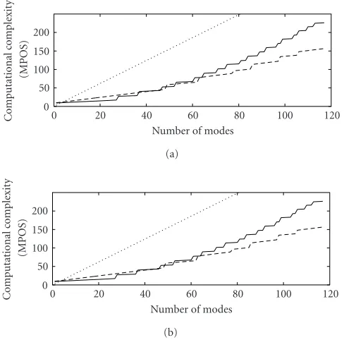
Figure 6 shows the dependency of the computational complexities on the number of simulated modes and thus the simulation accuracy or sound quality. The procedure used here to enhance the sound quality consists of sim-ulating more and more modes in consecutive order from the lowest mode on. Thus, the enhancement of the sound quality sounds like opening the lowpass in subtractive syn-thesis. The upper plot shows the computational complexi-ties for the linear system, simulated at audio rate and with the multirate approach using filter banks with P = 7 and

P = 15. The bottom plot shows the corresponding graphs for the nonlinear systems. It is assumed that the exter-nal forces only act on the string at one tenth of the out-put samples such that the weighting of the inout-puts do not have to be performed at each time instance. Thus, each lin-ear recursive system needs 3.1 MPOS for the calculation of one output sample, whereas the nonlinear system needs 4.2 MPOS.

It can be seen that the multirate implementations are much more efficient than the audio-rate simulations, except for simulations with very few modes. With all 117 simulated modes, the relation between audio rate and multirate sim-ulations (P = 7) is 363 MPOS to 157 MPOS for the linear system and 492 MPOS to 187 MPOS for the nonlinear sys-tem. This is a reduction of the computational complexity of more than 60%.

The steps in the multirate graphs denote the offset of the filter bank realization and that the interpolations of the fil-ter bank bands are only calculated as long as there is at least one mode simulated in those bands. On the one hand, the regions between the steps are steeper in the filter bank with

200 150 100 50 0

0 20 40 60 80 100 120

Number of modes

C

o

mputational

comple

xit

y

(MPOS)

(a)

200 150 100 50 0

0 20 40 60 80 100 120

Number of modes

C

o

mputational

comple

xit

y

(MPOS)

(b)

Figure6: Computational complexities of the FTM simulations dependent on the number of simulated modes at audio rate (dotted line), and with multirate approaches withP =7 (dashed line) andP =15 (solid line). (a): Linearly vibrating string, (b): vibrating string with nonlinear slap forces.

The second example shows the computational complex-ities of the simultaneous simulations of six independent strings as they occur in an acoustic guitar. Obviously, there is only one interpolation filter bank needed for all strings. The average number of simulated modes for each guitar string is assumed to be 60. In contrast to the first example, it is assumed that the modes are equally distributed in the fre-quency domain, such that at least one mode is simulated in each band.

Figure 7shows that the computational complexities de-pend on the choice of the used filter bank. On the one hand, each filter bank needs a fixed amount of computational cost which grows with the number of used bands. On the other hand, filter banks with more bands provide higher down-sampling factors for the production of the sinusoids which saves computational cost. Thus, the choice of the optimal filter bank depends on the number of simultaneously sim-ulated modes. For practical implementations this has to be estimated in advance.

It can be seen that for the linear case (solid line) the minimum computational cost is 272 MPOS using the filter bank with P = 11. In the nonlinear case, the filter bank withP =15 has the minimum computational cost with 319 MPOS for the simulation of all six strings. Compared to the audio-rate simulations with 1116 MPOS and 1512 MPOS for the linear and nonlinear case, respectively, the multirate sim-ulations allow computational savings up to 79%. Thus, the multirate simulations have a computational complexity of approximately 45 MPOS (53 MPOS) for each linearly (non-linearly) simulated string.

400

350

300

7 11 15 19

P

C

o

mputational

comple

xit

y

(MPOS)

Figure7: Computational complexities of the FTM simulations of a six-string guitar dependent on the number of bands for the multi-rate approach. Solid line: linearly vibrating string. Dashed line: vi-brating string with nonlinear slap forces.

7. CONCLUSIONS

The complete procedure of the FTM has been described from the basic physical analysis of a vibrating structure resulting in an initial boundary value problem via its analytical solution to efficient digital multirate implementations. The transver-sal vibrating dispersive and lossy string with a nonlinear slap force served as an example. The novel contribution is a thor-ough investigation of the implementation and the properties of a multirate realization.

It has been shown that the differences between audio-rate and multiaudio-rate simulations for linearly vibrating string simulations are not audible. The differences of the nonlin-ear simulations were audible but the multirate approach pre-serves the sound characteristics of the slap sound. The ap-plication of the multirate approach saves almost 80% of the computational cost at audio rate. Thus, it is nearly as efficient as the most popular physical modeling method, the DWG.

The multirate FTM is by far not limited to the example of vibrating strings. It can be used in a similar way to spatially multidimensional systems, like membranes or plates, or even to other physical problems like heat flow or diffusion.

ACKNOWLEDGMENTS

The authors would like to thank Vesa V¨alim¨aki for numer-ous discussions and his help in the filter bank design for the multirate FTM. Furthermore, the financial support of the Deutsche Forschungsgemeinschaft (DFG) for this research is greatly acknowledged.

REFERENCES

[1] C. Roads, S. Pope, A. Piccialli, and G. De Poli, Eds., Musical Signal Processing, Swets & Zeitlinger, Lisse, The Netherlands, 1997.

[2] L. Hiller and P. Ruiz, “Synthesizing musical sounds by solving the wave equation for vibrating objects: Part I,”Journal of the Audio Engineering Society, vol. 19, no. 6, pp. 462–470, 1971. [3] A. Chaigne and V. Doutaut, “Numerical simulations of

xy-lophones. I. Time-domain modeling of the vibrating bars,”

Journal of the Acoustical Society of America, vol. 101, no. 1, pp. 539–557, 1997.

[4] A. Chaigne, “On the use of finite differences for musical syn-thesis. Application to plucked stringed instruments,” Journal d’Acoustique, vol. 5, no. 2, pp. 181–211, 1992.

[5] A. Chaigne and A. Askenfelt, “Numerical simulations of pi-ano strings. I. A physical model for a struck string using finite difference methods,”Journal of the Acoustical Society of Amer-ica, vol. 95, no. 2, pp. 1112–1118, 1994.

[6] M. Karjalainen, “1-D digital waveguide modeling for im-proved sound synthesis,” inProc. IEEE Int. Conf. Acoustics, Speech, Signal Processing, vol. 2, pp. 1869–1872, IEEE Signal Processing Society, Orlando, Fla, USA, May 2002.

[7] C. Erkut and M. Karjalainen, “Finite difference method vs. digital waveguide method in string instrument modeling and synthesis,” inProc. International Symposium on Musical Acoustics, Mexico City, Mexico, December 2002.

[8] C. Cadoz, A. Luciani, and J. Florens, “Responsive input devices and sound synthesis by simulation of instrumental mechanisms: the CORDIS system,” Computer Music Journal, vol. 8, no. 3, pp. 60–73, 1984.

[9] J. M. Adrien, “Dynamic modeling of vibrating structures for sound synthesis, modal synthesis,” inProc. AES 7th Inter-national Conference, pp. 291–299, Audio Engineering Society, Toronto, Canada, May 1989.

[10] G. De Poli, A. Piccialli, and C. Roads, Eds.,Representations of Musical Signals, MIT Press, Cambridge, Mass, USA, 1991. [11] G. Eckel, F. Iovino, and R. Causs´e, “Sound synthesis by

phys-ical modelling with Modalys,” inProc. International Sympo-sium on Musical Acoustics, pp. 479–482, Le Normant, Dour-dan, France, July 1995.

[12] L. Trautmann and R. Rabenstein, Digital Sound Synthe-sis by Physical Modeling Using the Functional Transformation Method, Kluwer Academic Publishers, New York, NY, USA, 2003.

[13] D. A. Jaffe and J. O. Smith, “Extensions of the Karplus-Strong plucked-string algorithm,” Computer Music Journal, vol. 7, no. 2, pp. 56–69, 1983.

[14] K. Karplus and A. Strong, “Digital synthesis of plucked-string and drum timbres,”Computer Music Journal, vol. 7, no. 2, pp. 43–55, 1983.

[15] J. O. Smith, “Physical modeling using digital waveguides,”

Computer Music Journal, vol. 16, no. 4, pp. 74–91, 1992. [16] J. O. Smith, “Efficient synthesis of stringed musical

instru-ments,” inProc. International Computer Music Conference, pp. 64–71, Tokyo, Japan, September 1993.

[17] M. Karjalainen, V. V¨alim¨aki, and Z. J´anosy, “Towards high-quality sound synthesis of the guitar and string instruments,” inProc. International Computer Music Conference, pp. 56–63, Tokyo, Japan, September 1993.

[18] M. Karjalainen, V. V¨alim¨aki, and T. Tolonen, “Plucked-string models, from the Karplus-Strong algorithm to digital waveg-uides and beyond,”Computer Music Journal, vol. 22, no. 3, pp. 17–32, 1998.

[19] R. Rabenstein, “Discrete simulation of dynamical boundary value problems,” inProc. EUROSIM Simulation Congress, pp. 177–182, Vienna, Austria, September 1995.

[20] L. Trautmann and R. Rabenstein, “Digital sound synthesis based on transfer function models,” inProc. IEEE Workshop on Applications of Signal Processing to Audio and Acoustics, pp. 83–86, IEEE Signal Processing Society, New Paltz, NY, USA, October 1999.

[21] L. Trautmann, B. Bank, V. V¨alim¨aki, and R. Rabenstein, “Combining digital waveguide and functional transformation methods for physical modeling of musical instruments,” in

Proc. Audio Engineering Society 22nd International Conference on Virtual, Synthetic and Entertainment Audio, pp. 307–316, Espoo, Finland, June 2002.

[22] E. Rank and G. Kubin, “A waveguide model for slapbass syn-thesis,” inProc. IEEE Int. Conf. Acoustics, Speech, Signal Pro-cessing, pp. 443–446, IEEE Signal Processing Society, Munich, Germany, April 1997.

[23] M. Kahrs and K. Brandenburg, Eds., Applications of Digital Signal Processing to Audio and Acoustics, Kluwer Academic Publishers, Boston, Mass, USA, 1998.

[24] L. Trautmann and R. Rabenstein, “Stable systems for nonlin-ear discrete sound synthesis with the functional transforma-tion method,” inProc. IEEE Int. Conf. Acoustics, Speech, Signal Processing, vol. 2, pp. 1861–1864, IEEE Signal Processing So-ciety, Orlando, Fla, USA, May 2002.

[25] B. Girod, R. Rabenstein, and A. Stenger, Signals and Systems, John Wiley & Sons, Chichester, West Sussex, UK, 2001. [26] R. V. Churchill,Operational Mathematics, McGraw-Hill, New

York, NY, USA, 3rd edition, 1972.

method,” Signal Processing, vol. 83, no. 8, pp. 1673–1688, 2003.

[28] N. H. Fletcher and T. D. Rossing, The Physics of Musical In-struments, Springer-Verlag, New York, NY, USA, 1998. [29] L. Trautmann and V. V¨alim¨aki, “A multirate approach to

physical modeling synthesis using the functional transforma-tion method,” inProc. IEEE Workshop on Applications of Sig-nal Processing to Audio and Acoustics, pp. 221–224, IEEE Signal Processing Society, New Paltz, NY, USA, October 2003. [30] P. P. Vaidyanathan, Multirate Systems and Filter Banks,

Pren-tice Hall, Englewood Cliffs, NJ, USA, 1993.

[31] S. Petrausch and R. Rabenstein, “Sound synthesis by physical modeling using the functional transformation method: Effi -cient implementation with polyphase filterbanks,” inProc. International Conference on Digital Audio Effects, London, UK, September 2003.

[32] B. Bank, “Accurate and efficient method for modeling beating and two-stage decay in string instrument synthesis,” inProc. MOSART Workshop on Current Research Directions in Com-puter Music, pp. 134–137, Barcelona, Spain, November 2001.

L. Trautmannreceived his “Diplom-Inge-nieur” and “Doktor-Inge“Diplom-Inge-nieur” degrees in electrical engineering from the University of Erlangen-Nuremberg, in 1998 and 2002, re-spectively. In 2003 he was working as a Post-doc in the Laboratory of Acoustics and Au-dio Signal Processing at the Helsinki Uni-versity of Technology, Finland. His research interests are in the simulation of multi-dimensional systems with focus on digital

sound synthesis using physical models. Since 1999, he published more than 25 scientific papers, book chapters, and books. He is a holder of several patents on digital sound synthesis.

R. Rabenstein received his “Diplom-Inge-nieur” and “Doktor-Inge“Diplom-Inge-nieur” degrees in electrical engineering from the University of Erlangen-Nuremberg, in 1981 and 1991, respectively, as well as the “Habilitation” in signal processing in 1996. He worked with the Telecommunications Laboratory of this university from 1981 to 1987 and since 1991. From 1998 to 1991, he was with the Physics Department of the University of