R E S E A R C H
Open Access
A novel time of arrival estimation algorithm
using an energy detector receiver in MMW
systems
Xiaolin Liang
1*, Hao Zhang
1,2, Tingting Lyu
1, Han Xiao
1and T. Aaron Gulliver
2Abstract
This paper presents a new time of arrival (TOA) estimation technique using an improved energy detection (ED) receiver based on the empirical mode decomposition (EMD) in an impulse radio (IR) 60 GHz millimeter wave (MMW) system. A threshold is employed via analyzing the characteristics of the received energy values with an extreme learning machine (ELM). The effect of the channel and integration period on the TOA estimation is evaluated. Several well-known ED-based TOA algorithms are used to compare with the proposed technique. It is shown that this ELM-based technique has lower TOA estimation error compared to other approaches and provides robust performance with the IEEE 802.15.3c channel models.
Keywords:Empirical mode decomposition (EMD), Impulse radio (IR), Energy detection (ED), Millimeter wave (MMW), Time of arrival (TOA)
1 Introduction
Accurate estimation of the time of arrival (TOA) in wire-less systems is a challenging problem due to inter-symbol interference and multipath fading. Sixty gigahertz milli-meter wave (MMW) is a promising technology for accur-ate TOA estimation due to its unique advantages which include high time resolution [1], high multipath resolution [2], and robustness to interference [3]. In the 60-GHz fre-quency band, an energy detector (ED) receiver is preferred for TOA estimation because it can be implemented easily in hardware and does not require precise channel estima-tion and synchronizaestima-tion as with a matched filter (MF) [4]. As shown in Fig. 1, a conventional ED only consists of a band-pass filter (BPF), a squaring operator, an integrator, and a decision device.
The TOA can be estimated based on the first energy sample to exceed a threshold. Various ED-based TOA
estimation methods have been proposed [5–11]. Guvenc
first proposed a TOA estimation method via analyzing the kurtosis characteristics of the energy of the received pulses [6]. To account for signal variations, a normalized
threshold was employed in [7], which is based on the maximum and minimum energy values. In [8], a fixed threshold based on the maximum energy value was used. The cell averaging constant false alarm rate (CA-CFAR) method is developed for the TOA estimate by employing the ED receiver in [9].A weighted ED receiver was proposed in [10] to reduce the effects of noise. Although an extreme learning machine was used to obtain the threshold [11], this algorithm performs poorly with a con-ventional ED in low signal-to-noise ratio (SNR) environ-ments, particularly when there are noise-only energy values. We can see all of these algorithms perform poorly in low SNR environments because of the sensitivity of the threshold to noise. Using a conventional ED, these obtained energy samples are only noise which will have a significant effect on the TOA estimationτ^TOA.
To reduce the effects of noise and improve the estima-tion accuracy, in this paper, (1) an improved ED receiver was presented for TOA estimation which employs im-pulse radio (IR) 60 GHz MMW signals. The received signals were processed based on empirical mode decom-position (EMD) [12]. This method has been used to analyze non-stationary and nonlinear signals [13]. EMD adaptively decomposes a signal into a series of intrinsic mode functions (IMFs) in descending order of frequency
* Correspondence:[email protected]
1Department of Electronic Engineering, Ocean University of China, Laoshan
District Song Ling Road 238th, Qing Dao, People’s Republic of China Full list of author information is available at the end of the article
and a residual trend mode [13]. The IMFs and residual trend mode can be used to represent the noise which can then be deleted, resulting in an improved SNR [14]. (2) An ED-based TOA estimation technique was pro-posed which employs extreme learning machine (ELM). ELM was used to resolve a regression problem with the characteristics of the received ED values as inputs and the detector threshold as the output. Results are pre-sented which show that this de-noising approach pro-vides superior performance with the IEEE 802.15.3c channel models compared to several well-known tech-niques. And the simulation results were presented which show that ELM can provide robust and reliable TOA es-timates. Further, the proposed approach can be used with other wireless systems.
The remainder of this paper is organized as follows: Section 2 presents the system model. An improved ED receiver was discussed using EMD in Section 3. Section 4 discusses the signal characteristics, and the proposed ED-based TOA estimation technique is introduced in Section 5. Some performance results are given in Section 6, and Section 7 provides some conclusions.
2 System model
The IEEE 802.15.3c Line of Sight (LOS) and Non-line of Sight (NLOS) channel models have been proposed by the TG3c group for 60 GHz indoor residential, office, and library environments [21]. Several types of signals have been considered for 60 GHz systems [18]. Pulse position modulation (PPM) with a truncated sinc pulse has been shown to better conform to the Federal Com-munications Commission (FCC) regulations and provide a lower error probability than other signals. Thus, PPM with a truncated sinc pulse is considered here.
The received 60-GHz MMW signal can be expressed as:
where Eb is the energy per bit, (*) denotes convolution,
Nsis the number of pulses transmitted per data symbol,
j is the frame index, and Ts is the frame duration.
The time-hopping codes are cj∈(0, 1, .…,Nh−1),
where Nh =Ts/Tc is the number of chip positions in
a frame and the chip duration is Tc, β is the PPM
time shift employed when aj = 1 and there is no
shift when aj = 0, n(t) is the additive white Gaussian
noise (AWGN) with zero mean and two-sided power spectral density N0/2, and h(t,ϕ) is the channel realization from the triple Saleh-Valenzuela model in the IEEE 802.15.3c standard.
The transmitted pulse sequence in (1) is:
s tð Þ ¼
The channel realization can be given by:
h tð;ϕÞ ¼αLOSδðt;ϕÞ
where δ(⋅) denotes the Dirac delta function, L denotes the cluster number, and Kl denotes the rays number in
thelth lth cluster. The scalar αk, l denotes the complex
amplitude, αk, l and τk, l denote the TOA, and ωk, l
de-notes the azimuth of the kth ray in thelth cluster. The average TOA and the average AOA of the lth cluster can be expressed asTlandΘl, respectively.
The first term in (4) denotes the LOS component with
αLOS¼20 log10
andPLddenotes the path loss,λdenotes the wavelength,
ANLOSdenotes the attenuation caused due to the NLOS Fig. 1Block diagram of a conventional energy detector receiver
propagation, μd denotes the average range, Γ0 denotes the reflection coefficient, and h1 and h2 denote the heights of the transmitted antenna and the received an-tenna, respectively. Gt1, Gt2, Gr1, and Gr2 denote the gains of the transmitted antenna for the path 1 and path 2 and the gains of the received antenna for the path 1 and path 2, respectively.
The ED integrator output for a received signalr(t) can be expressed as:
where Ns is the number of pulses per symbol,Tbis the
integration duration, 3 Ts/2 is the integration interval,
Nb = 3 Ts/2 Tbis the number of samples,jis the frame
index, and the frame duration isTs. The TOA estimate
can be expressed as:
whereηis the threshold which is based on a normalized thresholdηnormgiven by:
ηnorm ¼
η − minðz nð ÞÞ
maxðz nð ÞÞ − minðz nð ÞÞ ð9Þ
As min(z[n]) is typically the integration of only noise, this can have a detrimental effect on the receiver
performance due to it is sensitivity to noise. In this paper, an extended threshold crossing (ETC) algorithm is proposed where the thresholdηcan be expressed as:
η¼ηnorm maxðz n½ Þ −
The problem is then how to obtainηnorm. Both
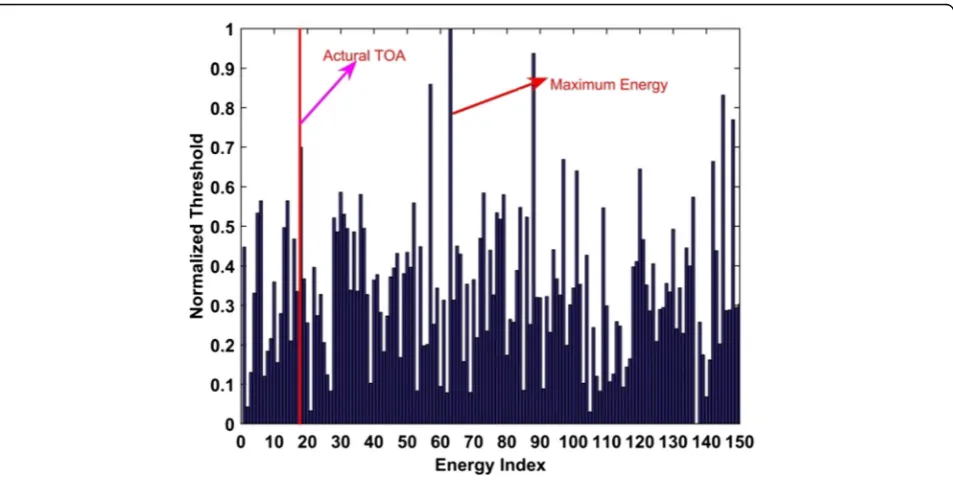
curve-fitting and fixed threshold (FT) have been employed, but these methods cannot provide precise TOA estimates because the first arriving signal component cannot be accurately determined. The simplest threshold selection was the maximum energy selection (MES) method, i.e., the maximum energy was considered as the threshold. As shown in Fig. 2, the actual TOA locates before the maximum energy, which is challenging to acquire due to the first arriving path which cannot be detected. As a re-sult, the MES method cannot achieve precise TOA esti-mations as shown in Fig. 2.
3 Proposed ED receiver
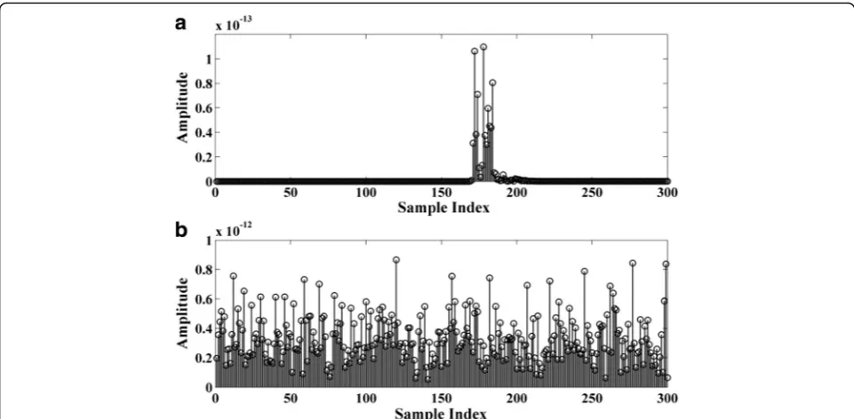
Figure 3 shows the energy values for a 60-GHz MMW signal (1) with the 3c CM1.1 model for an SNR of 10 dB and the signal without noise. These results indicate that many energy values are only noise which will have a sig-nificant effect on ^τTOA. To reduce the effects of noise and improve the estimation accuracy, an improved ED receiver based on EMD will be presented in this section.
Figure 4 shows the proposed receiver with signal de-noising using EMD. EMD adaptively decomposes the
received signal into N IMFs, i.e., IMF1, ..., IMFN, in descending frequency order and a residual trend mode. The residual trend mode is the difference be-tween the signal and the IMFs. The noise can be es-timated using the first few IMFs and the residual trend mode [17, 18].
To obtain the IMFs of a signal using EMD, letr(t) be the received signal, α(t) the residual component, m(t) the shifted component, IMFv(t) the vth IMF, and ru(t) (rl(t)) the upper (lower) envelope using a cubic spline function according to the local extrema.
The EMD algorithm is as follows [13]:
1) Setv= 0 andα(t) = r(t); 2) Letm(t) = α(t);
3) Determine the local extrema (maximum and minimum) ofm(t);
4) Construct the upper and lower envelopes of the extrema using cubic spline functions;
5) Determine the average envelope given by [14]:
u tð Þ ¼ruð Þ þt rlð Þt
2 ð11Þ
6) If the average envelope is zero or has only one extrema or zero crossing, go to step 7. Otherwise, calculate [15]:
m tð Þ ¼m tð Þ−u tð Þ ð12Þ
and go to step 3.
a
b
c
Fig. 4Block diagram of the new energy detector receiver
Fig. 3The energy values for a 60-GHz signal with the CM1.1 channel model.a60 GHz signal without noise andb60 GHz signal with AWGN and SNR = 10 dB
7) Ifα(t) is monotonic, stop. Otherwise, setv=v+ 1, IMFv(t) =m(t), andα(t) = r(t)−IMFv(t) and go to step 2 [16].
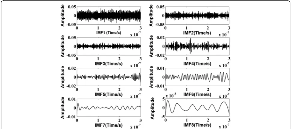
A 60-GHz MMW signal (1) with the 3c CM1.1 model and an SNR of 10 dB was decomposed using EMD into 11 IMFs and a residual trend mode. The first eight IMFs are shown in Fig. 5.
The boundary between the noise and signal compo-nents is determined as:
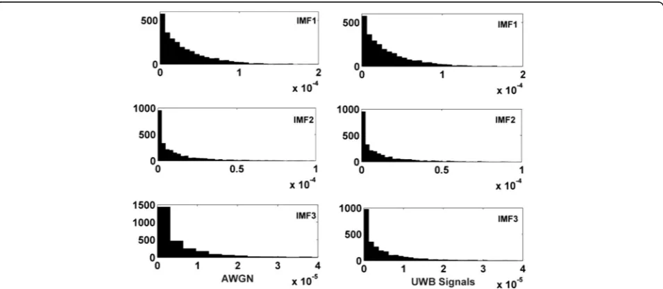
For a signal in AWGN, (14) is approximately a con-stant [17, 18]. As a result, IMFvcan be regarded as noise when RPv< 1 [18]. It was determined by simulation that IMFs 1 to 3 can be considered as noise. The histograms
of the first three IMFs of white Gaussian noise and the 60-GHz signal (1) with the CM1.1 model and SNR =
10 dB are shown in Fig. 6. IMF1for the 60-GHz MMW
and AWGN follow the bimodal distribution, and the other IMFs follow the Gaussian distribution. The corsponding histograms are presented in Fig. 7. These re-sults indicate that the first three IMFs have similar distributions in both cases. Table 1 shows the means and standard deviations of the first four IMFs, which confirm that the first three can be considered as noise [18]. Note that whenv> 3 the IMFs differ significantly.
The received signal can be approximated as:
^r tð Þ ¼X
11
v¼4
IMFvð Þt ð17Þ
And the noise estimated as:
^
n tð Þ ¼X
3
v¼1
IMFvð Þ þt h tð Þ ð18Þ
Thus, the noise energy is estimated in part B in Fig. 4 as:
And the signal energy values obtained in part C of Fig. 4 as:
z n½ ¼z1½ n−z2½ n ð20Þ
Figure 8 shows the energy values after de-noising using EMD with the 3c CM1.1 model and an SNR of 10 dB. The similarity, i.e., the energy values with strong amplitude between these results in Fig. 8 and Fig. 3a, confirms the effectiveness of EMD de-noising.
4 Energy signal characteristics
In this section, the curl of the energy values is
con-sidered. The other characteristics including the
kurtosis, skewness, maximum slope, and the standard deviation have been discussed in [11] in our previous work. However, the proposed threshold selection method cannot achieve accurate TOA estimations in low SNR values.
4.1 Curl
In vector calculus, the curl is an operator that de-scribes the infinitesimal rotation of a vector field. The maximum curl of the received energy values is
obtained as follows. Let (U, V) be a 2D vector field
with U=V and
Fig. 7Histograms of the energy value distributions for IMFs 1–3 of the AWGN and the 60-GHz signal plus noise in with the CM1.1 and SNR = 10 dB. The other parameters are the same as those in Section 4
Fig. 6Histograms of the IMFs for AWGN and a 60-GHz signal plus noise with the CM1.1 model and SNR =10 dB. The other parameters are the same as those in Section 4. The superimposed red lines are the Gaussian line fits for each IMF
U¼½z½ 1; z½ 2; z½ 3; …; z N½ b−1; z N½ b ð21Þ
The arraysXU andYVare the coordinates ofUand V,
respectively, and XU is an Nb×Nb dimensional array
given by:
XU¼
1; 2; 3; …; Nb−1; Nb
1; 2; 3; …;Nb−1; Nb
⋮ ⋮
1; 2; 3; …;Nb−1; Nb
1; 2; 3; …;Nb−1; Nb 2
6 6 6 6 6 4
3 7 7 7 7 7
5 ð
22Þ
YV is also an Nb×Nb dimensional array with YV
= (XU)T. Let the γth difference of the matrix U in the
YV(:, γ) direction beℜ(γ) and theγthdifference of the matrix V in the XU(γ, :) direction be ℑ(γ). The curl is then given by:
Cð Þ ¼γ ℑð Þγ − ℜð Þγ ð23Þ
The maximum curl is the maximum ofC(γ).
4.2 Signal parameter characteristics
In this section, the characteristics of the parameters of the energy values are investigated in indoor residential LOS
and NLOS scenarios for SNR within 4–30 dB. For each
SNR, 1000 channels were generated and the received
sig-nals sampled at 10 GHz. The system parameters areTs
= 200ns,Tb = 4ns,Tc = 1ns and^τU 0;Tf
, where
U(0,Tf) denotes the uniform distribution.
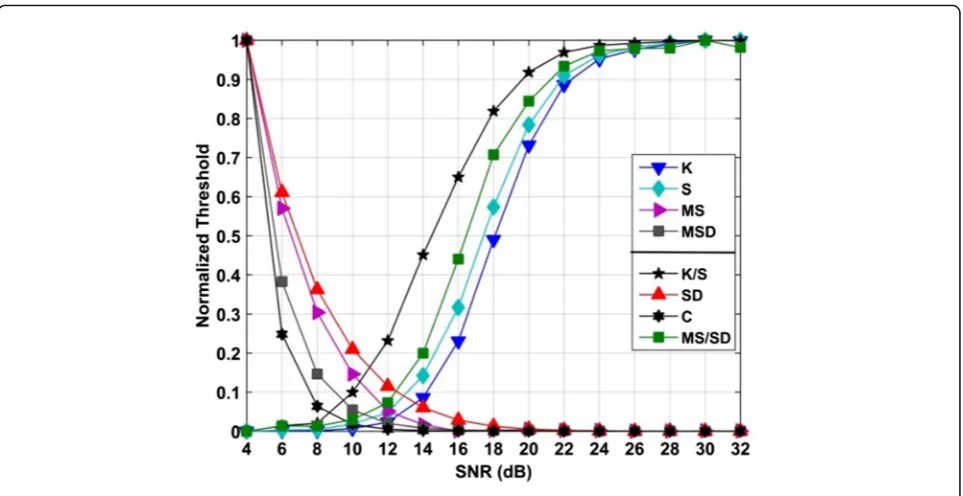
Figure 9 shows the skewness and maximum curl of the energy values. This figure also shows the kurtosis, max-imum slope, standard deviation, the ratios of the kurtosis to the skewness (K/S), the ratios of the maximum slope to the standard, and the products of the maximum slope and the standard deviation (MSD). These results show that the skewness and kurtosis increase as SNR in-creases, but the skewness changes more quickly. Con-versely, the maximum curl, maximum slope, and standard deviation decrease as SNR increases, but the maximum curl changes more quickly. Moreover, the skewness changes little while the maximum curl changes quickly when SNR < 8 dB. On the other hand, when
Fig. 8The energy values of the received signal after de-noising with the CM1.1 and SNR = 10 dB. The other parameters are the same as those in Section 4
Table 1The parameters for the acquired IMFs
IMF AWGN 60 GHz
Mean (× 10−4) Standard deviation Energy Mean (× 10−4) Standard deviation Energy
IMF1 6.99 0.0905 0.088 7.01 0.0905 0.088
IMF2 −0.80 0.0546 0.032 −0.71 0.0546 0.032
IMF3 2.36 0.0369 0.015 1.85 0.0366 0.019
SNR > 8 dB, the skewness changes rapidly but the max-imum curl has little change. As a result, these parame-ters cannot reflect a wide range of SNRs.
5 TOA estimation using machine learning
In this section, a new metric was proposed using the skewness and maximum curl of the energy samples. This metric can provide a better indication of the changes in SNR than the parameters considered in the previous sec-tion. Then, ELM is used to determine the relationship between this metric and the threshold values.
5.1 The new metric
The parameters presented in Section 3 are not suffi-ciently sensitive to changes over a wide range of SNRs. Thus, a new matric is presented in this section. The mean absolute error (MAE) of the TOA estimates is used to evaluate the TOA algorithms and is given by:
τMAE¼ 1
Nm XNm
m¼1
τm−^τm
½ ð24Þ
where τm and τ^m are the mth propagation time and
Fig. 10Average metric values with respect to SNR
Fig. 9The normalized parameters with respect to SNR
TOA estimate, respectively, and Nm is the number of
TOA estimates.
The MAE of the TOA estimation presented in [7] is less than that in [6] because the skewness changes more rapidly than the kurtosis when SNR > 12 dB. However, neither of these approaches can provide good perform-ance over a wide range of SNRs. Thus, a new metric is proposed which is given by:
J¼ ðK=SÞ−ðK=SÞmin K=S
ð Þmax−ðK=SÞmin
Q− C−Cmin Cmax−Cmin
R ð25Þ
where S is the skewness of the energy values and C is
the maximum curl of these values.SmaxandSminare the
maximum and minimum values of the skewness and
Cmax and Cmin are the maximum and minimum values
of the curl, respectively. Based on the extensive
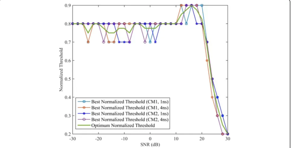
Fig. 12Optimum threshold with respect to the best threshold with different models andTb
simulation results, Q and R should be less than 20 and satisfyQ ≥ 3 R. In this paper,Q= 20 andR= 2.
To test the sensitivity of J with respect to SNR, the
average value of J was determined for the CM1.1 and
CM1.2 channel models with Tb= 1 and 4 ns. Figure 10
shows that J is a monotonic function of SNR and is
more sensitive to SNR than the other parameters over the range of SNRs.
5.2 Threshold determination
To find the best normalized thresholdηbest, the
relation-ship between MAE and ηnorm with respect to J, the
channel, and the integration period are examined.
Ex-cept for small values of J, the MAE decreases with
in-creasing J and the minimum MAE decreases with
increasing J. Figure 11 shows the relationship between
the normalized threshold and the MAEs. Usually, the normalized threshold with the minimum MAE was
referred as the best normalized threshold. The value of
ηnormfor the minimum MAE is defined as the best nor-malized thresholdηbest. As shown in Fig. 12, the average
ηbestis defined as:
Niis the number of integration periods andiis the in-tegration period in nanosecond.
The integration periods considered are 1 and 4 ns, so that
Artificial neural networks (ANN) such as the support vector machine (SVM) and back propagation neural net-work (BPNN) has been widely employed to solve
regres-sion problems [18–22]. ELM is a new and efficient
method to train a single-hidden-layer feedforward neural networks (SLFNs) [23]. ELM has been applied in many fields such as signal and information processing due to the good general performance and fast learning with
minimal human intervention [23–33]. ELM has been
shown to provide better results than SVM and require less training time than BPNN. The most important property is that the parameters in the hidden layers can be automatically determined and a simple generalized inverse operation can be used to obtain the output weight. Further, the only parameter that needs to be spe-cified is the number of nodes in the hidden layer [24]. Due to the complexity of the indoor channel environ-ment, it is very difficult to estimate TOA accurately using traditional curve-fitting methods. ELM can be used to resolve this problem by determining the rela-tionship between the input and output parameters ac-cording to the training results.
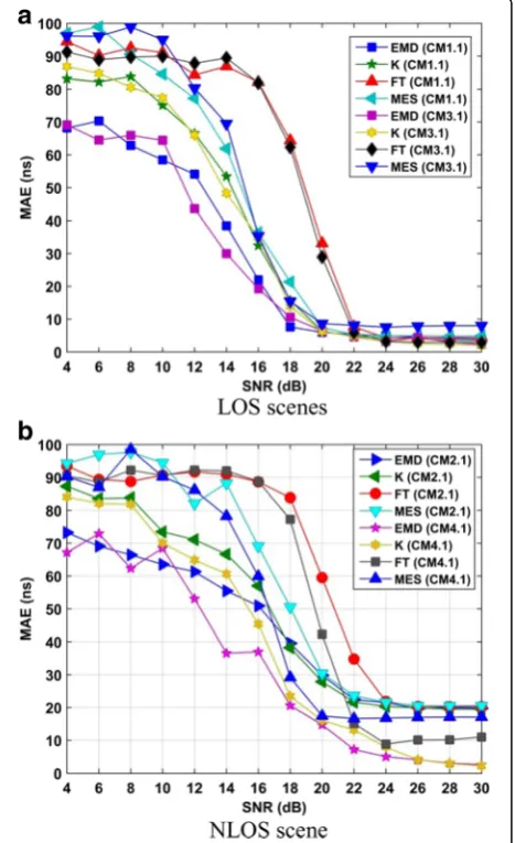
In ANN and SVM, the parameters in different layers need to be tuned which can consume significant time. Fig. 13The MAEs of several well-known methods with respect to
SNR.aLOS scenes.bNLOS scene
Further, the learning rate and learning epochs must be tuned through an iterative procedure which makes it difficult to obtain optimal values [23, 24]. Different from NN and SVM solutions, ELM is a tuning-free algorithm. The input weights and hidden bias can be generated randomly before training the SLFN based on the sample set.
In this paper, ELM is used to determine the
relation-ship between J and ηopt. The number of nodes in the
hidden layer is determined based on the training accur-acy. The root mean square error (RMSE) was calculated for 1000 training trials for each number of nodes. The results obtained show that the RMSE is a decreasing
function of the number of nodes, but when this number is 30, the RMSE is approximately constant. As a result, the number of node in the hidden layer is set to 30. The values J are rounded to the nearest integer or half inte-ger, and these rounded values are used in training the ELM. Asηoptvaries from 0 to 1, the sigmoid function is used as the activation function which is given by:
r¼ 1
1þe−x ð30Þ
6 Results and discussion
In this section, the MAEs of several well-known TC methods were examined for SNRs in the range 4 to 30 dB with the IEEE 802.15.3c channel models. Fig-ure 13a shows the calculated MAEs of the obtained TOA estimations with the LOS propagation including the channel models CM 1.1 and CM 3.1, while the MAEs of the obtained TOA over the channel models CM 2.1 and CM 4.1 were shown in Fig. 13b.
Based on the obtained results, the following conclu-sions can be obtained:
(1)The obtained MAEs of the new proposed ED receiver with respect to each given SNR within 4–30 dB indicate the excellent capability of removing the AWGN and show better performances on TOA estimations compared with several well-known algorithms based on the ED receiver whether in LOS or NLOS scene for each given integration period as shown in Fig.14.
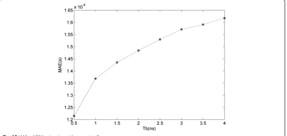
Fig. 15MAEs of TOA estimation with respect toTb
(2)The obtained MAEs of the improved ED received indicate that the ability to achieve TOA estimations in LOS models is better than that in NLOS models with regard to each given SNR within 4–30 dB. The difference is 15 ns at best.
(3)Integration periods usually can cause bad effects on TOA accuracy; the TOA estimation accuracy increases with the increasing integration period regardless of the propagation environment as shown in Fig.15. In the majority of cases, the MAEs with Tb= 1 ns is less than that withTb= 4 ns and the
difference is at most 2 ns.
(4)It was turned out that the new ED receiver was independent of the propagation models and integration periods.
Here, ELM denotes the new ED method with the optimum thresholds acquired with the ELM algorithm, MES denotes the maximum energy selection method, K denotes the kurtosis based method, and FT denotes the fixed normalized threshold. In all cases, the average MAE of the improved ED receiver with the ELM algo-rithm is the lowest among the above algoalgo-rithms.
7 Conclusions
In this paper, an improved energy detector (ED)-based TOA estimation method for impulse radio (IR) 60 GHz wireless system was presented using the empirical mode decomposition (EMD). The proposed solution employs the curl, the kurtosis, and the skewness of the energy values with an extreme learning machine (ELM). The optimum thresholds were determined for the IEEE 802.15.3c channel models in both LOS and NLOS envi-ronments. Results were presented which show that the proposed ELM approach provides better performance than other ED-based TOA estimation methods.
Acknowledgements
This work was funded by the Nature Science Foundation of China (41527901), Major Program of China’s Second Generation Satellite Navigation System (GF**********03), Fundamental Research Funds for the Central Universities (201713018), National High Technology Research and Development Program of China (2012AA061403), National Science and Technology Pillar Program during the Twelfth Five-year Plan Period (2014BAK12B00), National Natural Science Foundation of China (61501424), National Natural Science Foundation of China (61701462), Ao Shan Science and Technology Innovation Project of Qingdao National Laboratory for Mar-ine Science and Technology (2017ASKJ01), and the Qingdao Science and Technology Plan (17-1-1-7-jch).
Authors’contributions
XL conceived and designed the experiments, performed the experiments, analyzed the data, and wrote the paper. HX helped to carry out the experiment and analyzed the data. HZ, TL, and TAG helped to review and revise the whole paper. All authors read and approved the final manuscript.
Competing interests
The authors declare that they have no competing interests.
Publisher’s Note
Springer Nature remains neutral with regard to jurisdictional claims in published maps and institutional affiliations.
Author details
1Department of Electronic Engineering, Ocean University of China, Laoshan
District Song Ling Road 238th, Qing Dao, People’s Republic of China.
2
Department of Electrical Computer Engineering, University of Victoria, 3800 Finnerty Road Victoria BC, Victoria V8P 5C2, Canada.
Received: 6 September 2017 Accepted: 30 November 2017
References
1. N Leonor, R Caldeirinha, T Fernandes, et al., A simple model for average reradiation patterns of single trees based on weighted regression at 60 GHz, IEEE T. Antenn Propag63(11), 5113–5118 (2015)
2. T Nishesh, R Thipparaju, A switched beam antenna array with butler matrix network using substrate integrated waveguide technology for 60 GHz wireless communications. Int J Electron Commun.70, 850–856 (2016) 3. T Sakamoto, S Okumura, R Imanishi, et al., Remote heartbeat monitoring
from human soles using 60 GHz ultra-wideband radar. IEICE Electron Expr
12(21),1-6 (2015)
4. R Hazra, A Tyagi, A survey on various coherent and non-coherent IR-UWB receivers. Wireless Pers Commun79(3), 2339–2369 (2014)
5. X Liang, H Zhang, T Lu, et al., Energy detector based TOA estimation for MMW systems using machine learning. Telecommun Syst.64(2), 417–427 (2017)
6. I Guvenc, Z Sahinoglu, Threshold selection for UWB TOA estimation based on kurtosis analysis. IEEE Commun Lett.9(12), 1025–1027 (2005) 7. Guvenc, I., and Sahinoglu Z., Multiscale energy products for TOA estimation
in IR-UWB systems, in Proc. IEEE Global Telecommun. Conf., St. Louis, 209-213, 2005.
8. Guvenc, I., and Sahinoglu Z., Threshold-based TOA estimation for impulse radio UWB systems, in Proc. IEEE Int. Conf. on Ubiquitous Wireless Broadband, Zurich, 420-425, 2005.
9. A Maali, A Mesloub, M Djeddou, H Mimoun, G Baudoin, A Ouldali, Adaptive CA-CFAR threshold for non-coherent IR-UWB energy detector receivers. IEEE Commun. Lett.13(12), 959–961 (2009)
10. W Feng, T Zhi, BM Sadler, Weighted energy detection for noncoherent ultra-wideband receiver design. IEEE Trans Wirel Commun.10(2), 710– 720 (2011)
11. X Liang, H Zhang, T Lu, TA Gulliver, Extreme learning machine for 60 GHz millimeter wave positioning. IET Commun.11(4), 483–489 (2017) 12. T Wang et al., An EMD-based filtering algorithm for the fiber-optic SPR
sensor. IEEE Photon J8(3), 1-8 (2016)
13. H Zhang, F Wang, D Jia, et al., Automatic interference term retrieval from spectral domain low-coherence interferometry using the EEMD-EMD-based method. IEEE Photon. J8(3),1-9 (2016)
14. ZW Xu, T Liu, Vital sign sensing method based on EMD in terahertz band, EURASIP J. Adv Sig Pr2014(1)(2014) doi:10.1186/1687-6180-2014-75 15. YL Wu, BW Shen, An evaluation of the parallel ensemble empirical mode
decomposition method in revealing the role of downscaling processes associated with African easterly waves in tropical cyclone genesis. J Atmos Ocean Tech.33(8), 1611–1628 (2016)
16. Y Kopsinis, S McLaughlin, Development of EMD-based denoising methods inspired by wavelet thresholding. IEEE Trans. Signal Process.57(4), 1351– 1362 (2009)
17. Z Wu, NE Huang, A study of the characteristics of white noise using the empirical mode decomposition method. Proc R Soc A460, 1597– 1611 (2004)
18. R Chen, B Tang, J Ma, Adaptive denoising method based on ensemble empirical mode decomposition for vibration signal. J Vibration Shock
31(15), 83–86 (2012)
19. P Sunita, S Archana, PP Siba, A new training strategy for neural network using shuffled frog-leaping algorithm and application to channel equalization. Int. J. Electron. Commun.68, 1031–1036 (2014)
20. G Mahrokh, A Hamidreza, Performance analysis of neural network detectors in DS/CDMA systems. Int. J. Electron. Commun.57(3), 220–236 (2003) 21. K Fabian, The experimental results of the bulk-driven quasi-floating-gate
MOS transistor. Int. J. Electron. Commun.69, 462–466 (2015)
22. P Sotirios, S Katherine, Mobile radio propagation path loss prediction using artificial neural networks with optimal input information for urban environments. Int. J. Electron. Commun.69, 1453–1463 (2015)
23. G Huang, Q Zhu, C Siew, Extreme learning machine: a new learning scheme of feedforward neural networks, Proc. IEEE Int Joint Conf Neural Netw,2, 985-990 (2005)
24. L Shi, B Lu, EEG-based vigilance estimation using extreme learning machines. Neurocomputing102, 135–143 (2013)
25. Y Peng, WL Zheng, BL Lu, An unsupervised discriminative extreme learning machine and its applications to data clustering. Neurocomputing174(A), 250–264 (2014)
26. J Chorowski, J Wang, JM Zurada, Review and performance comparison of SVM-and ELM-based classifiers. Neurocomputing128, 507–516 (2014) 27. H Zhong, C Miao, Z Shen, Y Feng, Comparing the learning effectiveness of
BP, ELM, I-ELM, and SVM for corporate credit ratings. Neurocomputing128, 285–295 (2014)
28. XR Lee, CL Chen, HC Chang, Y Lee, A 7.92 Gb/s 437.2 mW stochastic LDPC decoder chip for IEEE 802.15.3c applications. IEEE T Circuits-I62(2), 507–516 (2015) 29. T Lu, Pulse waveforms for 60 GHZ M-ary pulse position modulation
communication systems. IET Commun.7(2), 169–179 (2013)
30. M Xia, W Lu, J Yang, et al., A hybrid method based on extreme learning machine and k-nearest neighbor for cloud classification of ground-based visible cloud image. Neurocomputing160, 238–249 (2015)
31. S Ding, H Zhao, Y Zhang, et al., Extreme learning machine: algorithm, theory and applications. Artif. Intell. Rev.44(1), 103–115 (2015)
32. JP Nobrega, ALI Oliveira, Kalman filter-based method for online sequential extreme learning machine for regression problems. Eng. Appl. Artif. Intell.
44, 101–110 (2015)