R E S E A R C H
Open Access
A limited feedback scheme for massive
MIMO systems based on principal component
analysis
Tiankui Zhang
1*, Anmeng Ge
1, Norman C. Beaulieu
1, Zhirui Hu
2and Jonathan Loo
3Abstract
Massive multiple-input multiple-output (MIMO) is becoming a key technology for future 5G cellular networks. Channel feedback for massive MIMO is challenging due to the substantially increased dimension of the channel matrix. This motivates us to explore a novel feedback reduction scheme based on the theory of principal component analysis (PCA). The proposed PCA-based feedback scheme exploits the spatial correlation characteristics of the massive MIMO channel models, since the transmit antennas are deployed compactly at the base station (BS). In the proposed scheme, the mobile station (MS) generates a compression matrix by operating PCA on the channel state information (CSI) over a long-term period, and utilizes the compression matrix to compress the spatially correlated high-dimensional CSI into a low-dimensional representation. Then, the compressed low-dimensional CSI is fed back to the BS in a short-term period. In order to recover the high-dimensional CSI at the BS, the compression matrix is refreshed and fed back from MS to BS at every long-term period. The information distortion of the proposed scheme is also investigated and a closed-form expression for an upper bound to the normalized information distortion is derived. The overhead analysis and numerical results show that the proposed scheme can offer a worthwhile tradeoff between the system capacity performance and implementation complexity including the feedback overhead and codebook search complexity.
Keywords: Massive MIMO, Limited feedback, Principal component analysis, Information distortion analysis
1 Introduction
The massive multiple-input multiple-output (MIMO) sys-tem which deploys large numbers of transmit antennas at the base station (BS) has been listed as one of the key techniques for fifth generation (5G) cellular networks [1]. The deployment of numerous antennas enables massive MIMO systems to achieve not only higher system capac-ity, but also higher spectrum and energy efficiency than conventional MIMO systems [2, 3].
The superior performance of the massive MIMO sys-tems relies on the spatial multiplexing and the minor multi-user interference. As is the case for conventional MIMO systems, this in turn requires the BS to have per-fect knowledge of the downlink channel state information
*Correspondence: [email protected]
1Beijing Key Laboratory of Network System Architecture and Convergence, School of Information and Communication Engineering, Beijing University of Posts and Telecommunications, No. 10, Xitucheng Road, Haidian District, 100876 Beijing, China
Full list of author information is available at the end of the article
(CSI) [4]. In a time division duplexing (TDD) system, the channel reciprocity can be exploited to acquire the down-link CSI at the BS [5]. However, things become more chal-lenging when the system operates in a frequency division duplexing (FDD) mode, where the channel reciprocity no longer holds. Therefore, a mobile station (MS) needs to feedback the downlink CSI through a rate-limited uplink channel. The authors in [6] drew the conclusion that the required feedback rate per user should be increased in proportion to the number of the transmit antennas for the sake of obtaining the full multiplexing gain. There-fore, feedback overhead turns into a key challenge in the massive MIMO systems.
The foundation of the works on feedback overhead reduction for MIMO systems is the correlation feature of MIMO channels. Limited feedback techniques for corre-lated MIMO channels were designed in [7–9]. A modified Grassmannian line packing codebook was proposed in [7], and the authors in [8, 9] rotated the codebook for i.i.d. channels with a unitary matrix to obtain the codebook for
correlated MIMO channels. A systematic codebook was designed for quantized beamforming in [10], which was implemented by maps that can rotate and scale spherical caps on the Grassmannian manifold.
Furthermore, a codebook for uniform rectangular arrays (URA) for massive MIMO antennas was designed in [11, 12]. It was derived by the Kronecker product of two ULA codebooks. The authors in [13] proposed a feedback framework for FDD massive MIMO systems that divides the coverage area into sub-sectors, where each sub-sector is formed by a set of narrow beams that covers a pre-assigned area in azimuth and elevation. Non-coherent trellis-coded quantization and trellis-extended codebooks for massive MIMO systems were proposed in [14, 15], which exploited a Viterbi decoder for CSI quantization and a convolutional encoder for CSI reconstruction. A projection based feedback compression was utilized to project the high-dimensional channel space into a lower dimensional subspace [16]. However, [16] did not explain how to feedback the projection matrix.
The compressive sensing (CS)-based limited feedback schemes for massive MIMO were proposed to reduce the feedback overhead by exploiting the spatial correla-tion of CSI [17–20]. The authors in [17] introduced CS to massive MIMO for limited feedback. A unique insight was provided that strong spatial correlations are exhib-ited in massive closely-packed antenna arrays, so channel vectors can be represented in sparse form in the spatial-frequency domain. Subsequently, a compressed analog feedback strategy for spatially correlated massive MIMO channels was proposed in [18]. In contrast to the strat-egy in [18], the low-dimensional CSI was quantized with a codebook and the preferred index was fed back in [19] and [20].
The choice of orthogonal basis, which is intended for the sparse representation of the original signal, plays an important role in the recovery of the original high-dimensional signal at the BS. Two such kinds of orthog-onal basis construction, the discrete cosine transform (DCT) and the Karhunen-Loeve transform (KLT), are usually employed [21]. If the channel correlation matrix is neither known at the MS nor the BS, the signal-independent DCT basis is a better option. On the one hand, because of its signal-independent nature, the uti-lization of the DCT basis does not require the MS to inform the BS of the channel correlation matrix. On the other hand, this makes the DCT basis incapable of track-ing the real-time change of channel state, which has a negative effect on system capacity. In contrast to the DCT basis, the KLT basis can excellently adapt to CSI change. Therefore, when MS and BS both know the instantaneous channel correlation matrix, the KLT basis can provide the optimal sparse representation, which promises accurate recovery even if only a small number of measurements
are available. Unfortunately, the signal-dependent nature of the KLT basis requests the MS to feedback channel cor-relation matrix instantaneously [22]. This can hardly be implemented in practical systems because of the heavy feedback overhead.
In this case, principal component analysis (PCA) can offer a tradeoff between system capacity and practical implementation [23, 24]. Compared with a DCT basis, PCA can be more adaptive to the change of the channel state, since PCA is signal-dependent [23]. This guarantees PCA better system capacity than a DCT basis. Com-pared with a KLT basis, PCA only needs that the MS and the BS have knowledge of the channel correlation matrix in a long-term period. This makes PCA achieve feedback overhead reduction much better than a KLT basis. What is more, the most attractive characteristic of PCA is that it is effective for dimensionality reduction of high-dimensional data [24], whose elements are cor-related. Inspired by this, PCA has great potential to be applied to the compression of high-dimensional CSI with strong spatial correlation to reduce feedback overhead in massive MIMO systems. To the best of our knowledge, there have not existed any works addressing a practical feedback scheme based on PCA.
This paper proposes a PCA-based feedback scheme for massive MIMO systems. In the proposed scheme, the MS utilizes a compression matrix, which is obtained by operating PCA on CSI observed over a long-term period, to compress spatially correlated high-dimensional CSI into low-dimensional representation. After quantizing the low-dimensional CSI with a random vector quantization (RVQ) codebook, the index of the preferred codeword is fed back to the BS in each short-term period. In order to track the channel changes and enable the BS to recover the high-dimensional CSI, it is necessary for the MS to refresh and feedback the compression matrix at every long-term period. Through the dimensionality reduction processing by PCA, feedback overhead and codebook search com-plexity can be reduced. The contributions of the paper are summarized as follows.
• A PCA-based feedback scheme for FDD massive MIMO systems is proposed. The operation
procedures at the BS and the MS are divided into two types, which are long-term period operations and short-term period operations. In more detail, the exact operation procedures both at the BS and the MS, as well as the derivation of the compression matrix at the MS, are presented. The distortion of the proposed scheme is analyzed. An upper bound to the normalized distortion is derived.
overhead and the codebook search complexity are analyzed and the system capacity performance is simulated. Looking at the simulation results and the feedback overhead analysis comprehensively, we draw the conclusion that our proposed scheme can achieve a compromise between system capacity and implementation complexity (feedback overhead and codebook search complexity).
The remainder of this paper is organized as follows. In Section 2, the massive MIMO system model is described. Section 2 first reviews the PCA method itself in Subsection and then provides the details of the proposed scheme in Subsection . Moreover, distortion of the pro-posed scheme is analyzed in Subsection . The feedback overhead as well as codebook search complexity compari-son and numerical results follow in Section 4 and Section 5, respectively. Finally, the conclusion of this paper is presented in Secton 6.
Notation:Throughout this paper, upper and lower case boldfaces are used to describe matrix A and vector a, respectively. We denote the transpose and the conjugate transpose of matrixAor vectorabyAT(aT) andAH(aH). In addiction,A−1denotes the inverse of a square matrix.
2 System model
We consider a downlink massive MIMO system, where there is a single cell, in which the BS equipped with Nt
antennas servesKsingle-antenna MSs.
2.1 Spatially correlated massive MIMO channel
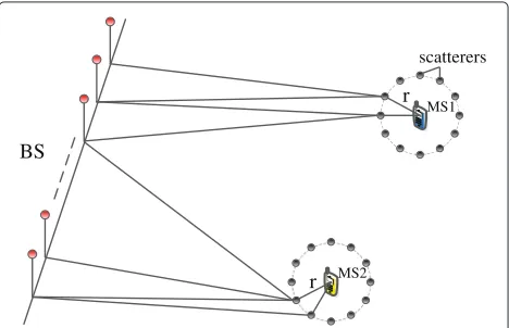
A massive MIMO broadcast channel is modeled in this section. For simplicity, but without loss of generality, a large-scale uniform linear array (ULA) with an enor-mous number of antenna elements deployed compactly is assumed. The spatial correlations are exhibited in the massive MIMO channel model, because of the insuffi-cient inter-element spacing. Additionally, a poor scat-tering environment may also contribute to the spatial correlation. Different from the previous works, which only consider either insufficient inter-element spacing or poor scattering environment, this paper combines the well-known Kronecker correlation model [25] with the geometrical one-ring model [26, 27], so as to describe the properties of the spatial correlation of the massive MIMO channel more precisely. Since the MS is equipped with a single antenna, the channel between thekthMS and BS is
denoted by a 1×Ntrow vectorhk(k=1, 2,. . .,K). Based
on the Kronecker correlation model,hkcan be modeled as
hk=hone−ringR
1 2
Tx, (1)
where R 1 2
Tx is the square root of the correlation matrix
at the transmitter depicting the impact of insufficient
inter-element spacing and hone−ring is derived from the
one-ring model describing the spatial correlation caused by a scattering environment. Note that the correlation of the channel is time varying, due to the change of both the relative positions of scatterers and the correlation matrix at the transmitter.
In more detail, the uth row and the vth column entry of RTx (the correlation coefficient between the uth and
the vth elements within the BS transmit antenna array) obeys the zeroth-order Bessel function of the first kind correlation model [18], that is
ruv=J0
2πduv
λ
, (2)
where duv is the distance between the two antenna
ele-ments andλdenotes the carrier wavelength.
As to the one-ring model, we assume that each MS is surrounded byQscatterers, which are uniformly dis-tributed on a circle with the radiusr, as shown in Fig. 1. Thehone−ringcan be given as follows [27],
hone−ring=
1 √
Q
Q
q=1
hkq. (3)
In (3),hkqis the channel vector of the MSkover theqth
scattering path, as given by
hkq=
βkq1e−j2π
dkq1+r λ ,. . .,
βkqNte−
j2πdkqNt+r λ
ejϕkq,
(4)
wheredkqmis the distance between theqthscatterer of the
kth MS and themth(m=1, 2. . .,N
t) BS antenna, while
dkqm+rdenotes the path length from thekthMS to the
mth antenna via the qth path. Also,ejϕkq represents the random common phase resulting from either the random perturbations of the MS location or the phase shift due to
r
scatterers
MS1
MS2 r BS
the reflection of the scatterer, andβkqmdenotes the path
loss of theqthscattering path, which is modeled by
βkqm= α
dkqm+r
γ, (5)
whereαis a constant andγ is the path loss exponent.
2.2 Downlink signal model
In the downlink transmission, sk ∈C and wk∈CNt×1
denote the transmit signal with power constraint E|sk|2=1 and the column precoding vector intended for
the kth MS, respectively. In this paper, zero-forcing pre-coding is adopted to eliminate multiuser interference [28]. Also, letnkbe additive Gaussian noise with zero mean and
unit variance at the MSk. Then the received signal of the kthMS can be expressed as
yk =
Pt
Khkwksk
desired signal
+
k=k
Pt
Khkwksk+nk
interfering signal and noise
, (6)
where Pt is the total transmit power of the BS. Equal
power allocation is assumed with Pt
K being the power
distributed to each MS.
As seen in (6), yk contains two main terms. The first term is the desired signal, while the other is the interfer-ing signal and noise. From (6), we can derive the system capacity as
C=
K
k=1
log2
⎛ ⎜
⎝1+
Pt
K|hkwk|2 Pt
K
k=k
|hkwk|2+1
⎞ ⎟
⎠. (7)
3 Feedback scheme for massive MIMO
3.1 Review of principal component analysis
We suppose that there areadata samples, each of which containsbcharacteristics. Thebcharacteristics have com-plicated correlation relationships with each other, which makes it possible for dimensionality reduction with PCA. For convenience of description, let the a×b matrix X
denote the original data containing the a data samples. The key point of PCA is how to derive a b×l (l<b) compression matrix¯, which is utilized to compress the high-dimensional data a×b X into a low-dimensional a×lX¯ as follows,
¯
X=X¯, (8)
in which,¯ is composed ofl-dominating eigenvectors, the so-called principal components, which are selected from allbeigenvectors ofX.
For the sake of determining which components are to be selected, the concept of contribution rate is intro-duced. Consider a descending ordering of theb eigenval-ues λ1,λ2. . .,λb. Then, the contribution rate of the gth
eigenvalueλg is defined as bλg g=1λg
, while the cumulative
contribution rate of the topleigenvalues can be expressed
by
l g=1λg
b g=1λg
. Generally, when the cumulative contribution
rate of the chosenlprincipal components exceeds a cer-tain level, the information loss is acceptable.
Finally, the originalXcan be recovered fromX¯ by
ˆ
X= ¯X¯H. (9)
3.2 Proposed PCA-based feedback scheme
A PCA-based feedback scheme for massive MIMO is proposed in this subsection. In the proposed scheme, different operations at the MS and the BS have differ-ent time periods, long-term period Tl and short-term
period Ts. Every long-term period Tl contains several
short-term periods Ts. In every Ts, the MS utilizes the
compression matrix to compress high-dimensional CSI into low-dimensional representation. Then, the com-pressed low-dimensional CSI is quantized by the RVQ codebook and the index of the preferred codeword is fed back to the BS. Because of the signal-dependent nature of PCA, the compression matrix is derived by executing PCA on the CSI which is obtained through continuous channel estimation during a whole long-term period.
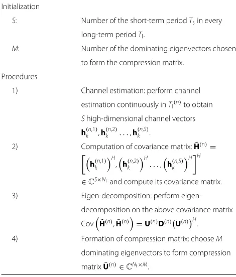
3.2.1 Compression matrix derivation
First of all, the detailed procedure for deriving the compression matrix in the nth long-term period Tl(n)
with the PCA method is given in Table 1. We assume MS k can obtain S high-dimensional channel vectors
h(kn,1),hk(n,2). . .,h(kn,S)
through ideal channel estimation
inTl(n). Here, theS channel vectors can be viewed asS
data samples, each of which containsNtcharacteristics. In
order to compress the high-dimensional CSI (channel vec-tors), we chooseM(MNt) dominating eigenvectors to
compose the compression matrixU¯(n)∈CNt×M.
The compression matrix obtained in the long-term period Tl(n) will be used by the MS to compress 1×Nt
channel vectors into 1×Mvectors, as well as by the BS to perform recovery in the periodTl(n+1).
3.2.2 MS operation
The main operations at the MS can be classified into two types: long-term period operations and short-term period operations.
Table 1Procedure of deriving the compression matrix in each long-term period with the PCA method at the MS
Initialization
S: Number of the short-term periodTsin every
long-term periodTl.
M: Number of the dominating eigenvectors chosen
to form the compression matrix.
Procedures
1) Channel estimation: perform channel
estimation continuously inTl(n)to obtain
Shigh-dimensional channel vectors
h(kn,1),hk(n,2). . .,h(kn,S).
2) Computation of covariance matrix:H˜(n)=
h(kn,1)H,h(kn,2)H. . .,h(kn,S)H
H
∈CS×Ntand compute its covariance matrix. 3) Eigen-decomposition: perform
eigen-decomposition on the above covariance matrix
CovH˜(n),H˜(n)=U(n)D(n)U(n) H
.
4) Formation of compression matrix: chooseM
dominating eigenvectors to form compression
matrixU¯(n)∈CNt×M.
Operation in thesth(s=1, 2. . .,S) short-term period of
thenthlong-term period,Ts(n,s), is described as follows:
Step 1. Channel estimation is performed to obtain a 1×Ntchannel vectorh(kn,s).
Step 2. Multiply h(kn,s) by the compression matrix derived in the previous long-term period
¯
hk(n,s)=hk(n,s)U¯(n−1). (10)
By this step, the original high-dimensional CSI (1×Nt)
is compressed into a low-dimensional representation (1×M). The compression ratio isNM
t.
Step 3.Quantize the low-dimensional CSIh¯(kn,s)by RVQ codebook and obtain the index number of the codeword that best fitsh¯(kn,s), that is
j(n,s)=arg max
j
h¯(kn,s)cj, (11)
wherecjis thejthcodeword of the codebook. Compared
with the quantizing high-dimensional CSI directly, the RVQ codebook used above can be designed to be much smaller. This not only reduces the feedback overhead, but also decreases the codebook search complexity.
Step 4.The index of the preferred codeword is fed back to the BS.
3.2.3 BS operation
Similarly, the main operation at the BS can also be clas-sified into long-term period operation and short-term period operation. At the end ofTl(n), the BS receives the compression matrix U¯(n) to perform high-dimensional CSI recovery in the next long-term periodTl(n+1). Mean-while, the short-term period operation follows the steps below:
Step 1. The codeword indexj(n,s) is received in each short-term period;
Step 2.As the BS and the MS share the same codebook, it is easy for the BS to find the quantized low-dimensional CSIhˆ(kn,s)by lettinghˆk(n,s)=cj(n,s);
Step 3.The high-dimensional CSI h
(n,s)
k can be
recov-ered by
h
(n,s)
k = ˆh( n,s)
k
¯
U(n−1)H, (12)
whereU¯(n−1)is derived from the periodTl(n−1).
3.3 Distortion analysis of proposed scheme
The distortion of our proposed scheme consists of three components, the distortion resulting from the PCA pro-cessing, the low-dimensional CSIh¯ quantization and the compression matrixU¯ quantization. To facilitate the dis-tortion analysis below, different representations of CSI in different stages are enumerated in Table 2.
3.3.1 Distortion analysis of PCA
First, we consider the distortion caused by the PCA method itself, with no quantization errors resulting from low-dimensional CSI or the compression matrix taken into account. That is, we measure the mean square error betweenhand h˜, where h˜ =hU¯U¯H. In this paper, his aNt dimensional row vector, which can be viewed as a
point in theNt dimensional space. Therefore, hcan be
Table 2Different representations of CSI in different stages
Representations Implications
h Original high-dimensional CSI estimated by MS
Low-dimensional CSI after normalization ¯
h and compression, that ish¯= hhUU¯¯
ˆ
h Quantized low-dimensional CSI
h High-dimensional CSI recovered fromhˆ
High-dimensional CSI recovered fromh¯ ˜
expressed by the linear combination of a set of orthogonal basis vectors,ui
h= Nt
i=1
αiui, (13)
whereuidenotes theithbasis vector.
In the PCA method, the high-dimensional CSI h is compressed into low-dimensional (M-dimensional)h¯, the components of which are derived by projectinghonto the Mdominating bais vectors. Given this, the reconstructed high-dimensional CSIh˜ can be modeled as the combina-tion ofMdominating basis vectors and the otherNt−M
less dominating vectors,
˜ h=
M
i=1
ziui+ Nt
i=M+1
biui. (14)
Therefore, the information distortion caused by the PCA itself, which is defined as the mean square error betweenhandh˜, can be expressed by
J= 1 S
S
n=1
hn− ˜hn2, (15)
where S denotes the number of short-term periods in a long-term period.
Proposition.The PCA-caused information distortionJ can be expressed by a linear sum ofNt−Mless
dominat-ing eigenvalues of the channel covariance matrix.
J=
Nt
i=M+1
λi.
Proof. See Appendix A.
3.3.2 Distortion analysis of quantization
According to [6], to measure the quantization error,h¯can be modeled as
¯
h=1−d2hˆ+de, (16)
wherehˆis the quantization ofh¯andeis a unit norm vector isotropically distributed in the nullspace ofhˆ. Parameter ddenotes the quantization error independent ofe, which satisfiesEd2≤2−MB−11. Here,Mrepresents the number of principal components andB1is the number of feedback
bits ofh¯. Similarly,U¯ can be modeled as
¯
U=1−D2Uˆ +DE, (17)
where Uˆ is the quantization of U¯ and E is composed of M unit norm vectors isotropically distributed in the
nullspace ofUˆ. Moreover, quantization error Dis inde-pendent ofUˆ satisfying
ED2≤2− B2/M
Nt−1, (18)
where B2 denotes the number of feedback bits of the
compression matrix.
Before analyzing the distortion between the original high-dimensional CSIhand the reconstructedh, we first focus on how to expresshin terms ofh.
Proposition.The reconstructed high-dimensional CSIh
can be expressed in terms ofhas
h= hU¯U¯
H−D2·hI
M−hU¯·d √
1−D2·eUˆH √
1−d2·√1−D2 ,
(19)
whereIM=
IM×M 0M×(Nt−M) 0(Nt−M)×M 0(Nt−M)×(Nt−M)
.
Proof. See Appendix B.
Having derived an expression for h in terms of h, our purpose is to analyze the distortion of the proposed scheme. We derive an upper bound to the normalized distortion (denoted by δ) between h and h. Instead of calculating δ directly, we first calculate the normalized
similarity (denoted byρ) betweenhandh. Then,δcan be conveniently obtained byδ=1−ρ.
Before calculating the normalized similarityρ between
h and h, it is insightful to look at the non-normalized
similarityEhh H
.
Proposition.A lower bound to the non-normalized sim-ilarity betweenhandhis given by
Ehh H
≥A−M·2−
B2/M
Nt−1 −A·2− B1
M−1, (20)
whereA=
Nt−
Nt
i=M+1
λi
Proof.Since we have derived an expression for h in terms of h, as given in Proposition 2, then the non-normalized similarity can be expressed by
Ehh H
=Eh
hU¯U¯H−D2·hIM−hU¯·d √
1−D2·eUˆH √
1−d2·√1−D2
H
=EhU¯2−D2·hIMHhH−hU¯·d·hU¯−DEeH √
1−d2·√1−D2
.
(21)
Now, because d2<1 and D2<1, √1−d2 and
√
1−D2 are also smaller than 1. Additionally, since the
quantization of low-dimensional CSI and the compression matrix are independent,EEeH=0. Therefore, the non-normalized similarity can be bounded by (22), shown at the top of the next page.
Ehh
H
≥E!hU¯2−D2·hIMHhH−hU¯·d·hU¯−DE eH
"
≥E!hU¯2−D2·hIMHhH−hU¯·d·h
¯
U−DE eH"
=E!hU¯2−D2·hIMHhH−hU¯·d·hUe¯ H
"
=E!hU¯2−D2·hIMHhH−hU¯2d2
"
=E!hU¯2"−ED2·EhIMHhH
−E!hU¯2"·Ed2
(22)
Further, we take advantage of the equations
E!hU¯2"=Nt−J, (23)
EhIMHhH=M, (24)
which are proved in Appendix C. Moreover, the upper
boundary of ED2 and Ed2 are 2− B2/M
Nt−1 and 2− B1 M−1, respectively. Consequently, we obtain (20).
From (23), we can observe that when there is no dis-tortion caused by PCA (J=0), as well as no quantization
error from low-dimensional CSI (2− B1
M−1 →0) or com-pression matrix (2−
B2/M
Nt−1 →0), the maximum value of the lower bound reachesNt. So the normalized similarity can
be expressed as
ρ≥ A−M·2 −B2/M
Nt−1 −A·2− B1 M−1 Nt
. (25)
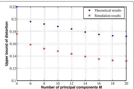
Finally, the upper bound of the normalized distortion of our proposed scheme can be obtained,
δ=1−ρ≤1−A−M·2 −B2/M
Nt−1 −A·2−MB−11 Nt
. (26)
According to the expression (26), we give the theo-retical upper bound of the distortion and the simulated distortion in Fig. 2.
4 6 8 10 12 14 16 18 20
0.1 0.12 0.14 0.16 0.18 0.2 0.22
Number of principal components M
Upper bound of distortion
Theoretical results Simulation results
Fig. 2Upper bound of distortion versus the number of principal components
4 Implementation complexity analysis
This section analyzes the feedback overhead and the code-book search complexity of the proposed scheme. For com-parison, the existing CS-based schemes utilizing the KLT basis and the DCT basis are also taken into account.
The number of feedback bits per user increases linearly with the number of transmit antennas, as modeled by [6]
B=(Nt−1)log2ρ≈
Nt−1
3 ρ, (27)
whereρdenotes the received signal-to-noise ratio (SNR) in decibels at the MS.
Consider a long-term period containing S short-term periods. When the proposed scheme is adopted, the num-ber of feedback bits can be represented by
Bpro=S(
M−1) ρ
3 +M
(Nt−1) ρ
3 , (28)
whereMis the number of the principal components, the first term denotes the number of feedback bits for quan-tizing low-dimensional CSI, and the second term is caused by the quantization of the compression matrix.
For the DCT-based CS scheme, there is no need for the MS to inform the BS of the channel correlation matrix, due to the signal-independent nature of the DCT basis. So the number of feedback bits for DCT-based CS is given by BDCT=S·(M−31)ρ.
BKLT=S·(
M−1) ρ
3 +S·Nt·
(Nt−1) ρ
3 . (29)
As for the codebook search complexity, it is propor-tional to the number of conjugate multiplications when searching for the best codeword. So the search complex-ity of the proposed scheme, DCT-based CS and KLT-based scheme in a long-term period can be expressed
as S·M·2(M−31)ρ +M·Nt·2( Nt−1)ρ
3 , S·M·2( M−1)ρ
3 and
S·M·2(M−31)ρ +S·Nt2·2( Nt−1)ρ
3 , respectively.
Table 3 illustrates the comparison in detail. Based on the analysis above, we can observe that the number of feedback bits and the codebook search complexity of the proposed scheme falls in between the DCT-based and KLT-based CS schemes.
5 Simulation results
In this section, we present simulation results. A single cell scenario is considered, where the BS deploys a uni-form linear array withNt=128 antennas servingK=6
single-antenna MSs. Table 4 lists the detailed simulation parameters.
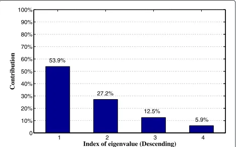
5.1 Feasibility validation
We verify whether PCA can be utilized to com-press spatially correlated high-dimensional CSI into low-dimensional representation. To achieve this purpose, we simulate the eigenvalue distribution of the spatially cor-related channels defined in (1). As shown in Fig. 3, the eigenvalue distribution of the spatially correlated chan-nel is far from uniform. The eigenvalues are sorted by their contribution rate in descending order. The contri-bution rate of the biggest eigenvalue exceeds 50 %, while the fourth biggest eigenvalue only contributes 5.9 %. The cumulative contribution rate of the top four eigenvalues exceeds 95 %. We can conclude that the spatially corre-lated channel vectors can be expressed by several principal components with low information distortion.
Table 3Comparison of feedback overhead and codebook search complexity
Table 4Simulation parameters
Parameters Assumption
Antenna configuration of BS ULA 0.5λspaced
Feedback channel Lossless & without delay
Carrier frequency 2.6 GHz
Bandwidth 10 MHz
Cell radius 200 m
Short-term period 1 ms
Long-term period 10 ms
Radius of scatterer ringr 10 m
Number of scatterersQ 10
Path loss exponentγ 2.5
Constantαin channel model 107
5.2 Evaluations of the proposed scheme
We show the simulation results of channel compression of the proposed scheme in Figs. 4 and 5. It is assumed that the SNR is 20 dB and there is no quantization error of the low-dimensional CSI.
Figure 4 shows the effect of the compression ratio
η= M Nt
on the system capacity. The comparison is among the proposed scheme, DCT-based CS and KLT-based CS. We can observe that whether in low or high compression ratio regimes, the KLT-based CS has the best performance, while the DCT-based CS performs the worst. To be emphasized, the best performance of the KLT-based CS is at a sacrifice of increased feedback over-head, as shown in Table 3. In this sense, the proposed scheme can offer a useful tradeoff. Additionally, as Fig. 4 shows, the proposed scheme performs much better than DCT-based CS in low compression ratio regimes.
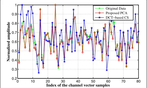
Figure 5 illustrates the recovery performance of the high-dimensional CSI at the BS under the circumstances that the BS has perfect knowledge of the low-dimensional
1 2 3 4
0 10% 20% 30% 40% 50% 60% 70% 80% 90% 100%
Index of eigenvalue (Descending)
Contribution
53.9%
12.5% 27.2%
5.9%
0.1 0.2 0.3 0.4 0.5 0.6 0.7 0.8 0.9 10
15 20 25 30 35 40 45
Compression ratio
System capacity (bps/Hz) Proposed PCA
DCT−based CS KLT−based CS
Fig. 4System capacity versus compression ratioη(SNR=20 dB, perfect quantization of low-dimensional CSI)
CSI without quantization. We take the proposed scheme and DCT-based CS for comparison. The 1×Nt original
CSI is compressed into 1×MCS low-dimensional
infor-mation, where MCS=20 and the compression ratio is
ηCS= MNCSt ≈0.16, while in the proposed scheme, the
number of principal components is MPCA=4 with the
compression ratio beingηPCA= MNPCAt ≈0.03.
As can be seen, the reconstructed high-dimensional CSI is considerably close to the original data when the PCA is utilized. But there still exists distortion because the PCA itself inevitably introduces information loss. How-ever, the recovery performance gets poorer in the case of the DCT-based CS. The reason is that the proposed scheme takes advantage of the signal-dependent nature of PCA, which makes it possible for the compression matrix to change adaptively in every long-term period according to the variation of the original data.
Figure 6 shows a system capacity (defined as the sum of all the users’ rates in the system) comparison. We choose four principal components to form the compres-sion matrix, so the comprescompres-sion ratio of PCA is 0.03. For reference, we first consider the ideal situation, where
0 10 20 30 40 50 60 70 80
0.2 0.3 0.4 0.5 0.6 0.7 0.8 0.9 1
Index of the channel vector samples
Normalized amplitude
Original Data Proposed PCA DCT−based CS
Fig. 5Recovery performance comparison between PCA and DCT-based CS
−100 0 10 20 30 40
20 40 60 80 100 120
SNR (dB)
System capacity (bps/Hz)
Perfect CSI
KLT−based CS (Perfect quantization) Proposed PCA (Perfect quantization) DCT−based CS (Perfect quantization) KLT−based CS (4 bits quantization) Proposed PCA (4 bits quantization) DCT−based CS (4 bits quantization)
Fig. 6System capacity comparison between PCA and other CS schemes
the BS can acquire perfect CSI with neither recovery dis-tortion nor quantization error. As illustrated in Fig. 6, the best system capacity can be achieved only when the BS acquires perfect CSI. Meanwhile, the proposed scheme outperforms the existing DCT-based CS scheme whether there is quantization error resulting from low-dimensional CSI or not. But, it performs a little poorer than the KLT-based CS scheme.
When we utilize the RVQ codebook to quantize low-dimensional CSI, the system capacity decreases in both cases because the quantization error must be taken into account. Based on the results in Fig. 6 and the feedback overhead analysis in Subsection 3.3, we can draw the con-clusion that our proposed scheme can offer a worthwhile design tradeoff between system capacity and feedback overhead.
6 Conclusions
Appendix
A Proof of Proposition 1
The PCA-caused information distortionJis
J= 1
In order to minimizeJ, we take partial derivatives with respect tozniandbiseparately, as given by
∂J
Similarly, when letting ∂∂bJ
i =0, we can also acquire
where h denotes the mean vector of all the S high-dimensional channel vectors estimated in a long-term period, as given by
Therefore,Jcan be re-expressed by
J= 1
In (38), the expression 1S
S
the covariance matrix ofhn, thenJcan be further given by
J=
Nt
i=M+1
uiChuiH. (39)
Our target is to minimize the PCA caused information distortionJ, which can be solved by the Lagrange Multi-plier (LM) method. After applying the LM, we can observe that the base vector must satisfy
ChuiH =λiuiH. (40)
Equation (40) indicates that base vector ui should be
chosen as the eigenvector of channel covariance matrix
Ch, andλiis the corresponding eigenvalue. As a result, the
PCA-caused information distortionJis
J=
B Proof of Proposition 2
As has been mentioned in Table 3,his the reconstructed high-dimensional CSI recovered fromhˆ, which is given by
h=hU¯· ˆhUˆH, (42)
¯
h= hU¯
hU¯. (43)
Substituting (16), (17) and (43) into (42), we can rewrite
has
Moreover, because of the independence betweenUˆ and
E, when multiplyingU¯ in (17) byEH, one obtains
Substitute (46) into (44), then (44) can be rewritten as
h= hU¯U¯
Uis composed of theMdominating eigenvectors, while Uis composed of the less dominatingNt−M
eigenvec-tors. In the proposed scheme, we only chooseM dominat-ing eigenvectors to compose compression matrixU¯, which is to be utilized to compress high-dimensional CSI into low-dimensional representation. Particularly, if choosing
all of the Nt eigenvectors, that is U¯ =U, the distortion
disappears, as given by
h=hUUH. (48)
into (48), and we can obtain
h=h
As mentioned above, the choice ofMdominating eigen-vectors inevitably leads to information distortion. Accord-ing to (49), the distortion caused by PCA can be expressed by
Because of the orthogonality betweenU¯ andU, one has
¯
UHU=0M×(Nt−M); (52)
UHU¯ =0(Nt−M)×M. (53) Therefore, Eq. (51) can be rewritten as
Eh2=E!hU¯U¯HU¯U¯HhH+hUUH2+
Since each element of channel vectorhobeys the Gaus-sian distribution with unit variance, thenEh2=Nt.
can be expressed by
where h(m)(m=1, 2,. . .M)denotes the mth element of
h. As mentioned above, each element of channel vec-torhobeys the Gaussian distribution with unit variance. Therefore,
EhIMHhH=M. (56)
Competing interests
The authors declare that they have no competing interests.
Funding
This work was supported by the NSF of China (No. 61271177 and No. 61461029) and Fundamental Research Funds for the Central Universities (2014ZD03-01).
Author details
1Beijing Key Laboratory of Network System Architecture and Convergence,
School of Information and Communication Engineering, Beijing University of Posts and Telecommunications, No. 10, Xitucheng Road, Haidian District, 100876 Beijing, China.2School of Communication Engineering, Hangzhou
Dianzi University, 310018 Hangzhou, China.3School of Science and Technology, Middlesex University, NW4 4BT, London, UK.
Received: 28 May 2015 Accepted: 12 May 2016
References
1. F Boccardi, RW Heath Jr., A Lozano, TL Marzetta, P Popovski, Five disruptive technology directions for 5G. IEEE Comm. Mag.52(2), 74–80 (2014) 2. F Rusek, D Persson, BK Lau, EG Larsson, TL Marzetta, O Edfors, F Tufvesson,
Scaling up MIMO: Opportunities and challenges with very large arrays. IEEE Sig. Proc. Mag.30(1), 40–60 (2013)
3. X Su, J Zeng, L-P Rong, Y-J Kuang, Investigation on key technologies in large-scale MIMO. J. Comput. Sci. Technol.28(3), 412–419 (2013) 4. X Rao, VKN Lau, Interference alignment with partial CSI feedback in MIMO
cellular networks. IEEE Trans. Sig. Proc.62(8), 2100–2110 (2014) 5. J Hoydis, S ten Brink, M Debbah, Massive MIMO in the UL/DL of cellular
networks: how many antennas do we need. IEEE Jour.Select. Areas in Comm.31(2), 160–171 (2013)
6. N Jindal, MIMO broadcast channels with finite-rate feedback. IEEE Trans. Info. Th.52(11), 5045–5060 (2006)
7. DJ Love, RW Heath Jr., Limited feedback diversity techniques for correlated channels. IEEE Trans. Vehicular Technol.55(2), 718–722 (2006) 8. P Xia, GB Giannakis, Design and analysis of transmit beamforming based on limited-rate feedback. IEEE Trans. Sig. Proc.54(5), 1853–1863 (2006) 9. J Choi, V Raghavan, DJ Love,Limited feedback design for the spatially
correlated multi-antenna broadcast channel,2013 IEEE Global Communications Conference (GLOBECOM), vol. 1, (Atlanta, GA, 2013), pp. 3481–3486
10. V Raghavan, RW Heath Jr., AM Sayeed, Systematic codebook designs for quantized beamforming in correlated MIMO channels. IEEE J. Select. Areas Commun.25(7), 1298–1310 (2007)
11. J Li, X Su, Z Zeng, Y Zhao, S Yu, L Xiao, X Xu,Codebook design for uniform rectangular arrays of massive antennas,Vehicular Technology Conference (VTC Spring), 2013 IEEE 77th, (Dresden, 2013), pp. 1–5
12. X Su, J Zeng, J Li, L Rong, L Liu, X Xu, J Wang,International Journal of Antennas and Propagation, vol. 2013. (Hindawi Publishing Corporation, New York, US, 2013)
13. D Ying, FW Vook, T Thomas, DJ Love,Sub-sector-based codebook feedback for massive MIMO with 2D antenna arrays,2014 IEEE Global
Communications Conference, (Austin, TX, 2014), pp. 3702–3707 14. J Choi, Z Chance, DJ Love, U Madhow, Noncoherent trellis coded
quantization: a practical limited feedback technique for massive MIMO systems. IEEE Trans. Commun.61(12), 5016–5029 (2013)
15. J Choi, DJ Love, T Kim, Trellis-extended codebooks and successive phase adjustment: a path from LTE-advanced to FDD massive MIMO systems. IEEE Trans. Wireless Commun.14(4), 2007–2016 (2015)
16. Y Han, S Wonjae, L Jungwoo,Projection based feedback compression for FDD massive MIMO systems,2014 IEEE Globecom Workshops (GC Wkshps), (Austin, TX, 2014), pp. 364–369
17. PH Kuo, HT Kung, PA Ting,Compressive sensing based channel feedback protocols for spatially-correlated massive antenna arrays,2012 IEEE Wireless Communications and Networking Conference (WCNC), (Shanghai, 2012), pp. 492–497
18. J Lee, SH Lee,A Compressed Analog Feedback Strategy for Spatially Correlated Massive MIMO Systems,Vehicular Technology Conference (VTC Fall), 2012 IEEE, (Quebec City, QC, 2012), pp. 1–6
19. P Cao, E Jorswieck,DCT and VQ based limited feedback in spatially-correlated massive MIMO systems,2014 IEEE 8th Sensor Array and Multichannel Signal Processing Workshop (SAM), (A Coruna, 2014), pp. 285–288 20. MS Sim, CB Chae,Compressed channel feedback for correlated massive
MIMO systems,2014 IEEE Globecom Workshops (GC Wkshps), (Austin, TX, 2014), pp. 360–364
21. W Lu, X Tan, Q Liu, Y Liu, D Wang, Compressive Channel Feedback Schemes Based on Redundant Dictionary in MIMO Communication Systems. Wireless Personal Communications.82(4), 2215–2229 (2015) 22. MS Sim, C-B Chae, inProc. IEEE Globecom Workshops (GC Wkshps).
Compressed channel feedback for correlated massive MIMO systems, (Austin, TX, 2014), pp. 327–332
23. JE Fowler, Compressive-projection principal component analysis. IEEE Trans. Image Process.18, 2230–2242 (2009)
24. LI Smith,A tutorial on principal components analysis. Technical report. (Cornell University, USA, 2002)
25. D Shiu, G Foschini, M Gans, J Kahn, Fading correlation and its effect on the capacity of multi-element antenna systems. IEEE Trans. Comm.48(3), 502–513 (2000)
26. J Nam, J-Y Ahn, A Adhikary, G Caire,Joint spatial division and multiplexing: realizing massive MIMO gains with limited channel state information,46th Annual Conference on Information Sciences and Systems(CISS 2012). (Princeton, NJ, USA, 2012)
27. H Yin, D Gesbert, L Cottatellucci, Dealing with interference in distributed large-scale MIMO systems: a statistical approach. IEEE Jour. Select. Topics Sig. Proc.8(5), 942–953 (2014)
28. A Wiesel, YC Eldar, S Shamai, Zero-forcing precoding and generalized inverses. IEEE Trans. on Sig. Proc.56(9), 4409–4418 (2008)
Submit your manuscript to a
journal and benefi t from:
7Convenient online submission
7Rigorous peer review
7Immediate publication on acceptance
7Open access: articles freely available online
7High visibility within the fi eld
7Retaining the copyright to your article