The generalized Bouguer anomaly
Kyozo Nozaki
Tsukuba Technical Research and Development Center, OYO Corporation, 43 Miyukigaoka, Tsukuba, Ibaraki 305-0841, Japan
(Received November 11, 2004; Revised June 28, 2005; Accepted September 20, 2005; Online published March 10, 2006)
This paper states on the new concept of the generalized Bouguer anomaly (GBA) that is defined upon the datum level of an arbitrary elevation. Discussions are particularly focused on how to realize the Bouguer anomaly that is free from the assumption of the Bouguer reduction densityρB, namely, theρB-free Bouguer anomaly, and on what is meant by theρB-free Bouguer anomalyin relation to the fundamental equation of physical geodesy. By introducing a new concept of the specific datum level so that GBA is not affected by the topographic masses, we show the equations of GBA upon the specific datum levels become free fromρB and/or the terrain correction. Subsequently utilizing these equations, we derive an approximate equation for estimatingρB. Finally, we show how to compute a Bouguer anomaly on the geoid by transforming the datum level of GBA from the specific datum level to the level of the geoid. These procedures yield a new method for obtaining the Bouguer anomaly in the classical sense (say, the Bouguer disturbance), which is free from the assumption ofρB. We remark that GBA upon theρB-free datum levelis the gravity disturbance and that the equation of it has a tie to the fundamental equation of physical geodesy.
Key words:Generalized Bouguer anomaly, Poincar´e-Prey reduction, specific datum level of gravity reduction, free-air anomaly, Bouguer reduction density.
1.
Introduction
In this paper, we present a new concept of the generalized Bouguer anomaly, which is defined upon the datum level of gravity reduction of an arbitrary elevation. The classi-cal Bouguer anomaly has been defined upon the geoid by the difference between the observed gravity reduced to the geoid and the reference gravity upon the geoid. The refer-ence gravity has been equated to the standard gravity (e.g. Heiland, 1946). No distinction was made between the refer-ence gravity and the standard gravity. In the theory of mod-ernphysical geodesy, the normal gravity upon the reference ellipsoid was introduced as the reference gravity (Heiska-nen and Moritz, 1967, p. 44). However, it is well known that the surface of the reference ellipsoid is different from that of the geoid. Therefore, the reference gravity upon the geoid is represented in terms of the normal gravity and the geoid height. Hackney and Featherstone (2003) recently discussed geodetic and geophysical ‘gravity anomalies’.
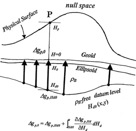
In order to perform the formulation, we attempted to gen-eralize the Bouguer anomaly upon an arbitrary elevation (the orthometric height). The reduction level laterally varies in height depending on the position of the gravity station. Also it does not coincide with a boundary of a Bouguer plate (or a Bouguer spherical cap) above the geoid. As is written in the text, we define the generalized Bouguer anomaly upon the datum level of an arbitrary elevation by the difference between the reduced observed gravity and the reference gravity that is reduced within the Earth’s
materi-Copyright cThe Society of Geomagnetism and Earth, Planetary and Space Sci-ences (SGEPSS); The Seismological Society of Japan; The Volcanological Society of Japan; The Geodetic Society of Japan; The Japanese Society for Planetary Sci-ences; TERRAPUB.
als by the Poincar´e-Prey reduction or, in short, the Prey re-duction (Heiskanen and Moritz, 1967, p. 146, pp. 163–165) from the normal gravity at the reference ellipsoid. The main aim of such a generalization of the Bouguer anomaly is to study the subsurface structures (e.g. Nozaki, 1997). The fig-ure of the Earth is not the subject of such a generalization of the Bouguer anomaly.
One of the most prominent features of the generalized Bouguer anomaly lies in the treatment of the reference grav-ity field: the use of the Prey reduction for the reference gravity. This means that the level of gravity reduction is within the Earth’s mass distribution outside the reference ellipsoid as well as inside.
In Section 2, we explain the motivations of this study. In Section 3, we describe the details of the formulation of the generalized Bouguer anomaly. Also, we explain the phys-ical properties of the new formula thus obtained. In Sec-tion 4, we define the three specific datum levels of grav-ity reduction: the one is the datum level so that the value of the generalized Bouguer anomaly becomes invariant for any Bouguer reduction density (the so-called ‘ρB-free da-tum level’), and the other is the datum level so that the sum of the terrain and Bouguer corrections becomes zero for any Bouguer reduction density. Also, we derive the generalized Bouguer anomaly at each specific datum level. Particularly, it will be shown that the generalized Bouguer anomaly upon theρB-free datum level, namely, theρB-free Bouguer anomaly, is free from the Bouguer reduction den-sity and is equal to the ‘gravity disturbance’ as defined in the physical geodesy. It will be also shown that the equa-tion of theρB-free Bouguer anomalyis the same as the fun-damental equation of physical geodesy, which defines the
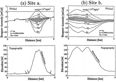
Fig. 1. Examples of the variation of the Bouguer anomaly distributions for Bouguer reduction densities. In the range of the Bouguer reduction densities
ρBs from 1.5×10³kg/m3to 2.5×10³kg/m3, the interval is 0.1×10³kg/m3.βdenotes the free-air gradient, DL the elevation of the datum level of gravity reduction. Arrows indicate Bouguer anomaly invariant (B A-invariant) points. Upper panels: Bouguer anomaly profiles, lower panels: topography profiles. The Site (a) profile shows an example in whichB A-invariant points occur. The site (b) profile shows an example in which
B A-invariant point does not occur.
‘gravity anomaly’ (Heiskanen and Moritz, 1967). In Sec-tion 5, we describe the details of the derivaSec-tion of an ap-proximate equation to be satisfied by the Bouguer reduction density and the anomalous vertical gradient of the gravity. This approximation can be used for the estimation of the Bouguer reduction density. In Section 6, using such an esti-mated Bouguer reduction density, we describe a method to obtain the generalized Bouguer anomaly distribution upon the geoid from that upon theρB-free datum level. We show that it is nothing but the Bouguer anomaly in the classical sense (say, the Bouguer disturbance) which has been used to study the subsurface structures.
2.
Motivations of the Approach
The most important motivation in this study is the ‘ex-istence of the Bouguer anomaly invariant point’. Figure 1 shows variation of Bouguer anomaly distributions due to the variation of the Bouguer reduction densityρB. The range ofρB variation is between 0.0 kg/m3 to 5,000 kg/m3. The Bouguer anomaly is defined upon the geoid as is done in a classical textbook (e.g. Heiland, 1946). Namely, the el-evation of the datum level of gravity reduction is taken at the geoid. The adopted free-air gradient is taken as 0.3086 mGal/m (10−5m/s2/m).
On Fig. 1(a), one can notice three points that are indicated by arrows. The Bouguer anomalies (BAs) for these points are independent of the variation of the Bouguer reduction
densitiesρB. For convenience, we call each of these points a ‘B A-invariant point’. On Fig. 1(b), no such B A-invariant points occur. What does such a B A-invariant point mean? At such a point, the Bouguer anomaly is free from the surrounding topographic masses.
Why do B A-invariant points exist? The reason is the elevation of the datum level of the gravity reduction. In this case, it is the geoid. If one changes the elevation of the datum level upwards and downwards, the location of the
B A-invariant points would also change. In other words, any gravity station can become a B A-invariant point for each gravity data by adjusting the elevation of the datum level.
If gravity anomalies are mapped by using only suchB A -invariant points, it could be the most useful one for studying subsurface structures, because the gravity anomalies are independent of the Bouguer reduction density ρB. From this point of view, the elevation of the datum level of the gravity reduction could have freedom to be selected.
3.
Formulation of the Generalized Bouguer
Anomaly
3.1 Height system and definition
data set are given by the observed gravity with position and elevation.
Although the exact determination of the orthometric height requires the complete knowledge of the actual grav-ity field within the topographic masses, this type of the height system is the most familiar one in the classical
Bouguer anomaly. Therefore, in deriving the concept of generalized Bouguer anomaly, we will use this height sys-tem. In Fig. 2(a), we show the correspondence between the height system used in this paper based on the orthometric height and the standard height system based on the normal height.
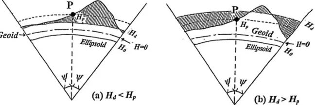
Here, we define the generalized Bouguer anomaly of the observed gravitygp. Let the elevation of an arbitrary datum
level beHp(orthometric height from the geoid). The
eleva-tion of the geoid is zero in this height system. The elevaeleva-tion of the datum level of gravity reduction isHd. The elevation
of the surface of the reference ellipsoid isH0. The vertical
Fig. 2. Height systems. (a) The orthometric height system. H: the orthometric height,N: the geoid height. SymbolsHp: the elevation (the orthometric height) of P,H0: the elevation of the ellipsoid, and
Hd: the elevation of the datum level of gravity reduction used in the text. (b) Normal height system. HN: the normal height (Torge, 2001, equation (3.107)),ζ: the height anomaly,h: the geometrical height (Heiskanen and Moritz, 1967) or the ellipsoidal height (Torge, 1989, equations (2.70a) and (2.71a);h=HN+ζ=H+N).
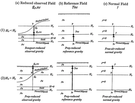
Fig. 3. Schematic illustration of the truncated spherical shell system of gravity correction. (a) For the case ofHd<Hp. (b) For the case ofHd>Hp. Hatching indicates the areas of mass-redistribution accompanied by the terrain and Bouguer corrections. Hp denotes the elevation of the gravity station P,Hd the elevation of the datum level of the gravity reduction,H0the elevation of the surface of the normal ellipsoid, andψthe truncation
angle of spherical gravity correction.
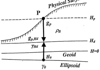
gradient of gravity (VGG) anomaly ∂g/∂r is included. The truncated spherical shell system of gravity correction is included by a truncation angleψ (see Fig. 3). Then, since the ‘anomaly’ can be defined by the difference between the observed value and the reference value, we define the gen-eralized Bouguer anomaly (gp,Hd) by the difference
be-tween the observed gravity reduced onto the datum level at an elevation Hd and the reference gravity reduced onto the
same datum level atHd. Namely, the generalized Bouguer
anomaly is defined by the form
gp,Hd :=gp,Hd−γHd, (1)
where,gp,Hd denotes the reduced observed gravity, andγHd
denotes the reference gravity. The detailed equations are described in Section 3.2. In Fig. 4, we show a schematic view of the observed gravity reduced onto an arbitrary da-tum level of elevation Hd and the reference gravity within
the mass distribution.
This approach of defining the generalized Bouguer anomaly at the same datum level looks classical. How-ever, in the followings, we will find a new relation be-tween the generalized Bouguer anomaly and the ‘gravity anomaly’ defined in the physical geodesy (Heiskanen and Moritz, 1967). In spite of the difference at the same datum level, we use the notationinstead ofδ. This is because we do not see the terminology ‘Bouguer disturbance’ in the literature.
3.2 Formulation
In this section, we discuss the generalized Bouguer anomaly based on the defining equation, Eq. (1). In the formulation, we express the generalized Bouguer anomaly
gp,Hd for the cases ofHd < Hp andHd > Hpseparately
to make their physical meanings clear, even though the both expressions are equivalent.
Symbols used in the formulation are summarized as fol-lows:
gp: observed gravity at a station P,
Hp: elevation of the gravity station,
Hd: elevation of the datum level of the gravity reduction,
Table 1. Definition of ‘correction’ and ‘reduction’.
Fig. 4. A conceptual illustration explaining the definition of the gener-alized Bouguer anomaly uponHd. gp,HdandγHd denote the reduced observed gravity and the reference gravity at the datum levelHd, re-spectively. The generalized Bouguer anomaly (gp,Hd) is defined by
gp,Hd = gp,Hd −γHd. ρB denotes the Bouguer reduction density. The reference gravity field is within the Earth’s mass distribution.
γ0: the normal gravity (upon the normal ellipsoid),
T Cp(1): the quantity of the terrain correction at the station
P for the unit density,
BCp(1): the quantity of the Bouguer correction at the sta-tion P for the unit density,
ρB: Bouguer reduction density,
T Cp: value of the terrain correction (=ρBT Cp(1)),
BCp: value of the Bouguer correction (=ρBBCp(1)),
F A: gravity anomaly in the physical geodesy or free-air anomaly in the Molodensky sense,
f: sum of the terrain and Bouguer corrections (=T Cp+ BCp),
G: Newtonian gravitational constant,
∂γ /∂r: VGG of the normal gravity field,
∂g/∂r: VGG anomaly defined by the difference between
the actual VGG after terrain and Bouguer corrections, and the normal VGG, which is compared at a point in the free-air space where the topographic masses of the densityρB are moved or removed by the terrain and Bouguer corrections,
r: the geocentric radial coordinate (positive upwards),
H±(1, ψ): sphericity factor for the spherical terrain and Bouguer corrections,
ψ: truncation angle of the spherical terrain and Bouguer corrections.
In the VGG anomaly∂g/∂r, the gravitational effect of the near surface density anomaly, which represents the inho-mogeneity of the topographic mass-density field fromρB, is included together with the VGG anomaly in the free-air space. The functionsH+(1, ψ)andH−(1, ψ), which gov-ern the gravitational behaviour of a thin spherical cap with a truncation angleψ(Nozaki, 1999), are given as
H±(1, ψ)=
1−cosψ
2 ±1, (2)
(hereafter, double signs should be taken in the same order). The derivation and the physical properties of these functions are shown in Appendix A. It is clear that an identical equation
H+(1, ψ)−H−(1, ψ)≡2 (3)
holds for any truncation angleψ. Concerning the spherical gravity corrections, see Nozaki (1981). Corresponding to the functionsH+(1, ψ)andH−(1, ψ), we distinguish the notation of the Bouguer correctionBCpforHd <Hpfrom
that forHd >Hp: BC+p denotes the Bouguer correction for Hd <HpandBC−p does that forHd >Hp, respectively.
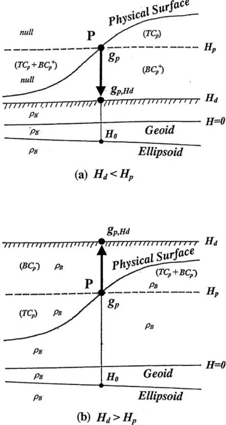
Fig. 5. Schematic illustration of the process to compute the reduced observed gravitygp,Hd. (a): Bouguer-reduced observed gravity for the case ofHd < Hp; the observed gravitygp is corrected by the terrain and Bouguer corrections (T CpandBC+p), then, reduced by the free-air reduction over the interval [Hp,Hd] as indicated by the arrow. (b): Prey-reduced observed gravity for the case ofHd > Hp; the observed gravitygpis corrected by the terrain and Bouguer corrections (T Cpand
BC−p), then, reduced by the Prey reduction over the interval [Hp,Hd] as indicated by the arrow. Mass-density distribution after the reduction for each case is shown in the figure.ρBis the Bouguer reduction density.
3.2.1 Reduced observed gravity (1)The case Hd <Hp
In this case, the observed gravitygp at the elevationHp
is reduced to the Bouguer-reduced observed gravitygp Hdat
the elevationHd(<Hp) as shown in Fig. 5(a).
When the elevation of the datum level of gravity reduc-tion Hd is lower than that of the gravity station Hp (see
Fig. 3(a)), the Bouguer correction is to remove the Earth’s materials above the datum level of gravity reduction. Ac-cordingly, we introduce the spherical Bouguer correction for Hd <Hpdenoted by
BC+p =
Hd
Hp
2πGρbH+(1, ψ)dr.
Then, in the case of Hd < Hp, the Bouguer-reduced
ob-served gravitygp,Hdupon the datum level of the gravity
re-ductionHd can be expressed as
gp,Hd =(gp+ f+)+ Hd
Hp ∂γ
∂r + ∂g
∂r
dr, (4)
where, f+ denotes the sum of the terrain and Bouguer corrections for the datum level ofHd <Hp:
f+=T Cp+BC+p
=ρBT Cp(1)+ Hd
Hp
2πGρBH+(1, ψ)dr. (5)
The Bouguer reduction (see Table 1) is made up of the spherical terrain correction (T Cp), the spherical Bouguer
correction (BC+p), and the free-air correction over the
inter-val [Hp,Hd]. Notice that, in the free-air correction, the term
of the VGG anomaly is added to the integrand on the right-hand side of Eq. (4). A schematic view of the Bouguer-reduced observed gravitygp,Hd for the case of Hd <Hpis
illustrated in Fig. 5(a). (2)The case Hd >Hp
In this case, as shown in Fig. 5(b), the observed gravity
gpat the elevationHpis reduced to the elevationHd(>Hp)
by the Prey reduction (e.g. Heiskanen and Moritz, 1967) after terrain and Bouguer corrections. When the elevation of the datum level of the gravity reductionHdis higher than
that of the gravity stationHp, the Prey reduction should be
applied over the interval [Hp,Hd] to the observed gravity gp (see also Fig. 3(b)). This is because we have to fill up
the open space above the Earth’s surfaceHpby the Bouguer
correction with the Earth’s materials whose density is ρB. Accordingly, we introduce the spherical Bouguer correction forHd >Hpdenoted by
BC−p =
Hd
Hp
2πGρBH−(1, ψ)dr.
Thus, in the case of Hd > Hp, we have the Prey-reduced
observed gravity,gp,Hd,
gp,Hd =(gp+ f
−)
+ Hd
Hp
2πGρB[H+(1, ψ)−H−(1, ψ)]
+∂γ ∂r +
∂g ∂r
dr, (6)
where, f− denotes the sum of terrain and Bouguer correc-tions for the datum level ofHd >Hp:
f−=T Cp+BC−p
=ρBT Cp(1)+ Hd
Hp
2πGρBH−(1, ψ)dr. (7)
Notice that the term of the Prey correction as well as that of the VGG anomaly are added to the integrand on the right-hand side of Eq. (6). A schematic view of the Prey-reduced observed gravity after terrain and Bouguer correctionsgp,Hd
Fig. 6. Correspondence of the reductions.; (a) the reduced observed gravity, (b) the Prey-reduced reference gravity, and (c) the normal gravity. Upper panels: the caseHd <Hp; lower panels: the caseHd > Hp. (a) The observed gravity at the station levelHpis reduced onto the datum levelHd. (b) The reduction of the reference gravity is done within the earth’s materials whose density isρB(Prey-reduction). (c) The reduction in the normal gravity field is done in the open or null space. The generalized Bouguer anomaly is defined by the difference between the Bouguer- or Prey-reduced observed gravity, and the Prey-reduced reference gravity.
the term 2πGρB[H+(1, ψ)−H−(1, ψ)] on the right-hand side of Eq. (6) is 4πGρB regardless ofψ(see Eq. (3)), we shall retain this form in the following sections to show ex-plicitly the gravitational contribution of the Bouguer spheri-cal cap. We notice here, the difference between Eqs. (5) and (7) is that the factor of the integrand on the right-hand side of Eq. (5) isH+(1, ψ), while in Eq. (7), it isH−(1, ψ).
3.2.2 Prey-reduced reference gravity The reference gravityγHd, at the datum levelHd, is defined in this paper
by the equation
γHd =γ0+ Hd
H0
2πGρB[H+(1, ψ)
−H−(1, ψ)]+∂γ
∂r
dr. (8)
The reference gravityγHd is reduced by the Prey reduction
from the normal gravityγ0, e.g. from the level H0 to the
levelHd. Here we applied the Prey reduction over the
inter-val [H0,Hd], instead of the Bouguer or free-air reduction.
This is because the reduction of the reference gravity from the levelH0to another level Hd should be done within the
Earth’s materials whose mass-density isρB. Thus, one can apply Eq. (8) both for the cases Hd > Hp andHd < Hp,
and even the case Hd < H0. We call the newly
intro-duced reference gravity the Prey-reintro-duced reference gravity. In Fig. 6, the correspondence between the Prey-reduced ref-erence gravityγHd, the reduced observed gravitygp,Hd, and
the normal gravity is schematically illustrated. The detailed explanation of the reference field is added in Appendix C.
3.2.3 Formula of the generalized Bouguer anomaly (1)The case Hd <Hp
When the elevation of the datum levelHd is lower than
that of the gravity station Hp, the formula of the
Bouguer-reduced observed gravity is given by Eq. (4). Substituting Eqs. (4) and (8) into Eq. (1) and arranging the terms with respect to the Bouguer reduction densityρB, we obtain the formula of the generalized Bouguer anomalygp,Hd, for
the case ofHd <Hp, as
gp,Hd =gp−γ0− Hp
H0 ∂γ ∂rdr+
Hd
Hp ∂g
∂r dr
+ρB
T Cp(1)+ Hd
Hp
2πG H+(1, ψ)dr
− Hd
H0
2πG[H+(1, ψ)−H−(1, ψ)]dr
The first and second terms in the braces of Eq. (9) are the contribution of the terrain and Bouguer corrections to the observed gravity for Hd < Hp, while the third term in
the braces is essentially that of the Prey correction to the reference gravity (see Eqs. (5) and (4)).
(2)The case Hd >Hp
When the elevation of the datum levelHd is higher than
that of the gravity station Hp, the formula of the
Prey-reduced observed gravity is given by Eq. (6). Substituting Eqs. (6) and (8) into Eq. (1) and arranging the terms with respect to the Bouguer reduction densityρB, we obtain the formula of the generalized Bouguer anomaly gp,Hd, for
the case ofHd >Hp, as
In the braces of Eq. (10), the first and second terms are the contribution of the terrain and Bouguer corrections to the observed gravity for Hd > Hp, while the third term
is essentially that of the Prey correction to the reference gravity. Notice, that the interval of integration of the Prey correction is not [H0,Hd] but [H0,Hp]. This is because,
when Hd > Hp, the term of the Prey reduction over the
interval [Hp,Hd] of the reduced observed gravity in Eq. (6)
is canceled out by subtracting that of the reference gravity in Eq. (8). At the same time, this corresponds to the fact that the mass-density above the station heightHpis zero for the
case ofHd >Hp.
3.3 Remarks about the generalized Bouguer anomaly 3.3.1 Unified expression of the formula of the gener-alized Bouguer anomaly The unified expression of the generalized Bouguer anomalygp,Hdcan be written in the
same form both forHd <Hpand forHd >Hp. By
arrang-This means that Eqs. (9) and (10) are equivalent each other. 3.3.2 Effect of the datum level change on the gen-eralized Bouguer anomaly When we regard the eleva-tion of the datum level Hd as an independent variable, the
changing rate of the generalized Bouguer anomalygp,Hd
with respect to the elevation of the datum level Hd can be
expressed by the equation
∂gp,Hd ∂Hd =
2πGρBH−(1, ψ)+∂g
∂r . (12)
This is directly derived from any one of Eqs. (9) and (10). In this paper, we will call this rate∂gp,Hd/∂Hd the
‘re-duction rate’. Equation (12) implies that, when we ignore the term∂g/∂r as is usually the case, the upward trans-formation of the datum level Hd brings the decrease of the
generalized Bouguer anomalygp,Hd at the reduction rate
of 2πGρBH−(1, ψ), andvice versa. Notice that the reduc-tion rate of Eq. (12) does not include the terms of the normal gravity field.
4.
Generalized Bouguer Anomaly at Some
Spe-cific Datum Level of the Gravity Reduction
In this section, we define the specific datum levels of the gravity reduction so that the generalized Bouguer anoma-lies are not affected by the topographic effects. Also we discuss the physical properties of the generalized Bouguer anomalies upon the specific datum levels.4.1 Specific datum levels of the gravity reduction 4.1.1 Specific datum levelHd0 The condition of the
specific datum level Hd0 of gravity reduction, upon which
the generalized Bouguer anomaly gp,Hd becomes
inde-pendent of anyρB (see Section 2 and Fig. 1), is given by the equation
∂gp,Hd
∂ρB =0. (13)
By this condition, one can obtain the defining equation of
Hd0from Eq. (9) or equivalently from Eq. (10) as
In the following we shall call this specific datum level of gravity reduction Hd0 ‘ρB-free specific datum level’ or in
short ‘ρB-free datum level’.
The meaning of theρB-free datum level Hd0can be
un-derstood as follows. The condition expressed by Eq. (13) corresponds to that the sum of the terms in the braces on the right-hand side of Eq. (9) or Eq. (10) is zero, i.e. inde-pendent of the Bouguer reduction densityρB.
4.1.2 Specific datum levels Hd1 and Hd2 Another
condition for defining the specific datum levels Hd1 and
Hd2, upon which the topographic gravitational effects are
eliminated, is given by Eqs. (5) and (7):
T Cp+BC±p =ρBT Cp(1)
+ Hd
Hp
2πGρBH±(1, ψ)dr =0. (15)
This is the condition that the sum of the terrain correction
T Cp and the Bouguer correction BCp is always zero
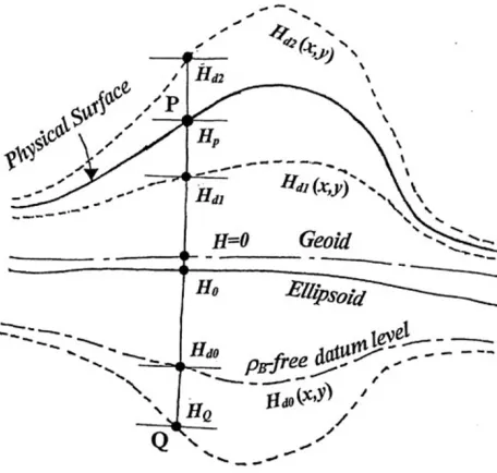
re-gardless ofρB. This condition leads to the definition of the additional specific datum levels (Hd1andHd2): Since the terrain correctionT Cp(1)is almost everywhere positive for a small truncation angle ψ (say ψ < 3 de-grees), the elevation of the specific datum level Hd1 is
Fig. 7. Geometric relation between the specific datum levelsHd0,Hd1and
Hd2. Each specific datum level spreads the surface with undulation as a
function of the horizontal coordinatesxandy:Hd0(x,y),Hd1(x,y)or
Hd2(x,y). For the flat Earth approximation, the specific datum levels
Hd1 andHd2 are located at the mirror-imaged positions with respect
to the elevation of the gravity stationHp (see Eq. (23)); and so the specific datum levelsHd1andHd0with respect to the elevation of the
normal ellipsoidH0(see Eq. (22)). The elevation of the pointQ(HQ) isHQ=2(Hp−H0)/H−(1, ψ)+Hp.
(Hd1 < Hp), and the elevation of the specific datum level Hd2 is almost everywhere higher than that of the gravity
stationHp(Hd2>Hp).
Notice that Hd1 and Hd2 can be computed from the
known quantity of the terrain correction for the unit density
T Cp(1)for each gravity station. Also Hd0 is computable
if H0 is given. Remember that H0 is the elevation of the
reference ellipsoid in the orthometric height system of this paper, and its magnitude is equal to the geoid heightN (i.e.
H0= −N).
4.1.3 Relation between the specific datum levels Since the specific datum levels Hd0, Hd1 and Hd2 can be
defined for each gravity station, these specific datum levels form surfaces as functions of the horizontal position (x,y):
Hd0=Hd0(x,y), Hd1=Hd1(x,y) and
Hd2=Hd2(x,y).
Each of the three surfaces of Hd0(x,y), Hd1(x,y) and
Hd2(x,y) has undulation like the Molodensky telluroid
(Heiskanen and Moritz, 1967).
The geometric relation among the surfaces of the specific datum levels Hd0(x,y), Hd1(x,y)andHd2(x,y)is shown
in Fig. 7. From Eqs. (14) and (16), the specific datum levels
Hd0andHd1are related toH0in the following way
H0= −H
−(1, ψ)Hd
0+H+(1, ψ)Hd1
2 . (18)
Also, from Eqs. (16) and (17), the specific datum levelsHd1
andHd2have a relation againstHpas
Hp =
H+(1, ψ)Hd1−H−(1, ψ)Hd2
2 . (19)
In the same manner, from Eqs. (14) and (17), the specific datum levelsHd0andHd2have a relation
Hd0=
2(Hp−H0)
H−(1, ψ) +Hd2. (20)
It is interesting that the relation between Hd0 for H0 and
Hd2forHpis reciprocal:
Hd2=
2(H0−Hp)
H−(1, ψ) +Hd0. (21) From Eqs. (18) and (19), we have the relation equivalent to Eq. (20) or Eq. (21):
2(Hp−H0)= −H−(1, ψ)(Hd2−Hd0).
Particularly in a flat Earth approximation of the gravity correction, i.e.,
H+(1, ψ)→ +1 and H−(1, ψ)→ −1 [forψ∼0, refer to Eq. (2)],
the specific datum levels Hd0 and Hd1 locate at the same
distance of lower and upper positions with respect to H0,
respectively (see Eq. (18)), resulting in
H0=
Hd0+Hd1
2 , (forψ∼0). (22) Also from Eq. (19), Hp takes the algebraic mean value of Hd1andHd2:
Hp =
Hd1+Hd2
2 , (forψ∼0). (23) Furthermore, if the topography is very gentle and hence the value of the terrain correctionT Cp(1)is negligibly small,
Hd0 degenerates into the elevationHQof the point Q, that
is,
HQ=Hp−2(Hp−H0)/H−(1, ψ)
as shown in Fig. 7 (see Eq. (14)). Also, Eq. (22) represents that Hd0 and Hd1 are at the mirror-image position of the
reference ellipsoid levelH0. Also, Eq. (23) represents that
Hd1 and Hd2 are at the mirror-image position of Hp, and
degenerate into Hpwhen T Cp(1)is negligibly small, (see
Eqs. (16) and (17)).
On the other hand, particularly in the spherical shell sys-tem of gravity correction, i.e.,
H+(1, ψ)→ +2 and H−(1, ψ)→ −0 [forψ=π, see Eq. (2)],
the datum levels Hd0 andHd2take the infinite values (see
Eqs. (14) and (17)), and lose their physical meanings, while
Hd1still takes a definite value of
Hd1=Hp−
T Cp(1)
4πG , (forψ=π) (24)
(see Eq. (16) forψ = π). At first sight, this seems to be inconsistent with Eq. (18). However, substituting Eq. (14) into Eq. (18), we get
H+(1, ψ)Hd1 =2H0+2(Hp−H0)+H−(1, ψ)Hp
−T Cp(1)
2πG , (forrψ=π).
4.2 Introduction of the new notationF A
gp: observed gravity at the elevationHp,
0
Hp
∂γ
∂rdr: free-air correction from the level of elevationHp
to the level of the geoid,
γ0: normal gravity upon the normal ellipsoid.
Note that the interval of integration [Hp,0] in Eq. (25-1)
and the interval [0,H0] in the interval [H0,Hp] in Eq. (9)
or (10) are complementary to each other with respect to the whole interval of the free-air correction. The integra-tion over the interval [H0,0] plays an important role in
the geodetic interpretation of F A(as is described in Sec-tion 4.5).
Ignoring the VGG anomaly, F A is the approximation of the free-air anomalygF (e.g. Heiskanen and Moritz,
1967, equation (3-62), p. 146). Alternatively, F Acan be rewritten as
where ζ is the height anomaly. This can be easily un-derstood by changing the interval of integration [0,Hp]
in Eq. (25-2) to [H0,Hp +H0], and assuming N (geoid
height) = ζ (height anomaly), and H (orthometric height)=HN(normal height):
Hp
In this case, it is not necessarily required that ∂γ /∂r is constant. Importantly, in this case, the integration (free-air correction) over the interval [Hp −ζ,Hp], which is
complementary to the interval of integration [−ζ,Hp−ζ]
in Eq. (26) for the whole interval [−ζ,Hp] ≈[H0,Hp] in
Eq. (9) or (10), plays essentially the same role as that over the interval [H0,0] as mentioned above.
Thus,F Aof Eq. (26) represents the new gravity anomaly (Heiskanen and Moritz, 1967, equation (8-7), p. 293), or the point free-air anomaly (e.g. Torge, 1989, equation (3-7a), p. 54), that is the difference between the measured gravity at the ground and the normal gravity at the telluroid. In this sense, F A is the free-air anomalies in the Molodensky’s sense, although F A of Eq. (25-1) was firstly defined for the free-air corrected observed gravity on the geoid as the gravity anomaly (Heiskanen and Moritz, 1967, equation (2-139), p. 83).
Using F A, hereafter, we will proceed to formulate the
ρB-free generalized Bouguer anomaly.
4.3 Representation of the generalized Bouguer anomaly at the specific datum level
The generalized Bouguer anomaly upon an arbitrary da-tum level of Hd is given by any one of Eqs. (9) and (10).
The first and second terms in the braces of Eq. (28) are essentially the terrain and Bouguer corrections for the ob-served gravity, while the third term in the braces is essen-tially the Prey correction for the reference gravity. As was previously mentioned, one can derive the same results by using Eq. (10) instead of Eq. (9).
SubstitutingHd0,Hd1andHd2(Eqs. (14), (16) and (17))
into Hd in Eq. (28), we have, respectively, the
representa-tion formulae of the generalized Bouguer anomalies at the specific datum levels of gravity reductionHd0,Hd1andHd2
Notice that, in Eq. (29), the sum of the terrain and Bouguer corrections (the first and second terms in the braces) is canceled out by the term of the Prey correction (the third term in the braces), resulting in all the terms con-cerningρB in the braces on the right-hand side vanish by setting the datum level atHd0. This is because the specific
datum level Hd0is so defined as to satisfy Eq. (13). Also,
in Eqs. (30) and (31), the sum of the terrain and Bouguer corrections, which corresponds to the first and the second terms in the braces on the right-hand sides, vanish by set-ting the datum levels atHd1andHd2, respectively. This is
because the specific datum levels Hd1 and Hd2 are so
de-fined as to satisfy Eq. (15). Notice, that the interval of inte-gration of the fifth term on the right-hand side of Eq. (31) is not [H0,Hd2] but [H0,Hp], because the mass-densityρB is
zero over the interval [Hp,Hd2].
When these vanishing terms in Eqs. (29), (30) and (31) are set to zero, we have the final equations
gp,Hd0 =F A−
Equation (32) is a representation of the condition that the generalized Bouguer anomaly (left-hand side of Eq. (9) or Eq. (29)) is independent of the Bouguer reduction density
ρB. Equations (33) and (34) are representations of the con-dition that the sum of the terrain and Bouguer corrections is zero regardless ofρB. Namely, by setting the datum level at the ρB-free datum level Hd0, the generalized Bouguer
anomalygp,Hd0results in being free from the Bouguer
re-duction densityρB. In this paper, we call this generalized Bouguer anomalygp,Hd0 the ρB-free Bouguer anomaly.
Also, by setting the datum levels Hd1 and Hd2, the
gen-eralized Bouguer anomaliesgp,Hd1 andgp,Hd2 result in
being free from the terrain and Bouguer corrections. The integrand of 2πGρB[H+(1, ψ)−H−(1, ψ)] in Eq. (33), as well as that in Eq. (34), corresponds to the Prey correction for the reference field.
Here we shall pay special attention to that Eqs. (32)–(34) yield the relation betweenF Aand the generalized Bouguer
anomaly at the specific datum level (gp,Hd0, gp,Hd1, or gp,Hd2), respectively.
4.4 The meaning of the generalized Bouguer anomaly at theρB-free datum levelHd0
In the simple case when the term of the VGG anomaly
∂g/∂r is sufficiently small, Eq. (32) of the generalized Bouguer anomaly at theρB-free datum level Hd0(gp,Hd0)
Rewriting Eq. (35) by using Eq. (25), we obtain the follow-ing approximate representations
gravity disturbance on the ellipsoid
=
gravity disturbance on the geoid
=
gravity disturbance at any datum levelHdc. (36)
Thus, we conclude that the generalized Bouguer anomaly at theρB-free datum level Hd0, that is, theρB-free Bouguer
anomalygp,Hd0, is the gravity disturbance. Also, Eq. (36)
represents that the gravity disturbance is invariant for the level transformation in the free-air space.
Equation (35) represents the relation between the gravity disturbance (gp,Hd0) and F A(the Molodensky’s free-air
anomaly). Although the details will be described in the next section, this fact suggests that Eq. (35) has a tie to the fundamental equation of physical geodesy. Also, Eq. (36) implies that the gravity disturbance in the free-air space can be defined not only at the elevation of the geoid but also at any level Hdc. The gravity disturbance (gp,Hd0) is not
defined by the right-hand side of Eq. (36) but results in the right-hand side of Eq. (36). Such a view of the gravity disturbance (gp,Hd0) is schematically illustrated in Fig. 8.
Particularly, whengp,Hd0is upward-continued in the
free-air space to the station level at P, it is interesting that the gravity disturbance (gp,Hd0at P) does not change the value
even though the removed or moved topographic masses are completely restored (cf. Eqs. (29) and (32)).
and
gp,Hd2 =gp,Hd0
− Hp
H0
2πGρB[H+(1, ψ)−H−(1, ψ)]dr
+ Hd2
Hd0 ∂g
∂r dr, (38)
respectively.
4.5 Relation to the fundamental equation of physical geodesy
SinceH0 = −N, it is shown below that Eq. (35) has a tie
to the fundamental equation of physical geodesy (Heiska-nen and Moritz, 1967, equation (2-148), p. 86).
Regarding VGG of the normal gravity field as constant, Eq. (35) yields
F A=gp,Hd0+(−H0) ∂γ
∂r. (39)
On the other hand, the fundamental equation of physical geodesy is written as
g = −∂T ∂r +
T γ
∂γ
∂r, (40)
where, g denotes the (geodetic) gravity anomaly, andT
denotes the gravity disturbing potential. Then, using the relation
δg= −∂T ∂r
and the Bruns’ formula
T =Nγ,
Fig. 8. Schematic illustration that represents the equivalence of the gen-eralized Bouguer anomaly at theρB-free datum level Hd0to the gravity
disturbance at any datum level. The VGG anomaly (∂g/∂r) is ne-glected here.Ndenotes the geoid height (N= −H0).
Eq. (40) is written as
g=δg+N∂γ
∂r, (41)
which is equivalent to the fundamental equation of physical geodesy. Comparing Eqs. (39) and (41), it is clear that these two equations are similar to each other, identifyingF Awith
g,gp,Hd0withδg, and−H0withN.
5.
Estimation of the Bouguer Reduction Density
We will show in this section that the Bouguer reduction densityρB is estimated by the plot of F Aagainst the spe-cific datum levels, and also H0 is estimated on the sameplot.
5.1 Derivation of the equation for estimating the Bouguer reduction density
As was explained previously, each of the specific da-tum levels Hd0, Hd1 and Hd2, upon which the
general-ized Bouguer anomaliesgp,Hd0,gp,Hd1,gp,Hd2are
de-fined, forms a surface as a function of the horizontal co-ordinates(x,y): Hd0 = Hd0(x,y), Hd1 = Hd1(x,y)and
Hd2=Hd2(x,y).
Here, we shall notice that Eqs. (32), (33) and (34), which represent the generalized Bouguer anomalies at the spe-cific datum levels, hold for every point of horizontal coor-dinates(x,y). Therefore, one can consider the differential quantities of the generalized Bouguer anomalies gp,Hd0, gp,Hd1, andgp,Hd2with respect to the specific datum
lev-els Hd0, Hd1 and Hd2 in the neighbourhood of (x,y),
re-spectively. In this case, it is necessary to differentiate not onlygp,Hd0,gp,Hd1,gp,Hd2 and F A, but also Hp and
T Cp(1), since they are functions of Hd0, Hd1andHd2that
are functions ofxandy.
Differentiating Eqs. (29), (30) and (31) with respect to
Hd0,Hd1andHd2, respectively, we have
dgp,Hd0
d Hd0
= d F A d Hd0
+
1− d Hp
d Hd0
∂g
∂r , (42)
dgp,Hd1
d Hd1 =
d F A d Hd1 +
1− d Hp
d Hd1
∂
g ∂r
−2πGρB[H+(1, ψ)−H−(1, ψ)], (43)
and
dgp,Hd2
d Hd2 =
d F A d Hd2 +
1− d Hp
d Hd2
∂
g ∂r −
d Hp d Hd2
2πGρB[H+(1, ψ)
−H−(1, ψ)]. (44)
As for the derivation of these equations, refer to Ap-pendix B.
In the above calculation, d Hp/d Hd0, d Hp/d Hd1 and
d Hp/d Hd2 are taken into account because Hd0, Hd1 and
Hd2are not independent variables but functions ofHp.
Be-sides, the elevation of a gravity stationHp is a function of
datum level (dgp,Hdi, fori=0,1,2) can be written as i.e. the lateral variation of gp,Hdi is sufficiently small,
Eq. (45) yields
Since the partial differential coefficients satisfy the equation
∂gp,Hd0
Eq. (46) leads directly to the following approximate rela-tion:
Thus, subtracting Eq. (42) from Eq. (43) and using Eq. (47), and assuming constant VGG anomaly, (∂g/∂r) = β,
From Eqs. (43) and (44), one can also derive the result equivalent to Eq. (48). We shall notice again that all quan-tities in Eq. (48) but forρBandβare known. Differential coefficients in Eq. (48) have the following relations:
d Hp
These relations of Eqs. (49) and (50) can be derived from Eq. (18).
When the VGG anomaly β is sufficiently small, Eq. (48) gives the following equation
ρB ≈
Thus, we have the final approximate equation, Eq. (51-1), for estimating the Bouguer reduction densityρB. Equation (51-1) means thatρBis calculated from the gradients ofF A
with respect to the specific datum levels. Concrete method for evaluating the gradients d F A/d Hd0 and d F A/d Hd1
will be described in the next section. The effect of the VGG anomaly (β) on the Bouguer reduction density estimation can be evaluated by Eq. (48).
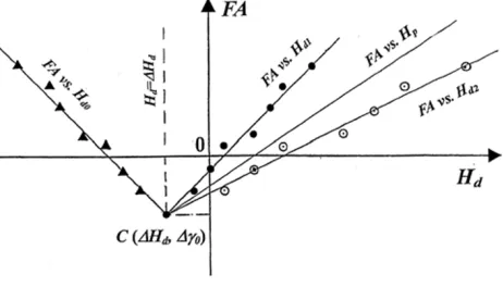
5.2 F Avs.Hd0,Hd1andHd2diagram
Each free-air anomaly F Ain Eqs. (32), (33) and (34), which is a computable quantity, is a function of each spe-cific datum level Hd0, Hd1 and Hd2, respectively. Here,
we plot the free-air anomaly (F A) against the datum level
Hd (e.g.Hd = Hd0, Hd1 or Hd2) for every gravity station.
Then, we obtain generally a set of plots as schematically shown in Fig. 9. In this paper, we call the diagram of these plots ‘F Avs.Hddiagram’.
The characteristics found in theF Avs. Hd diagram are
as follows:
(1) One can measure the gradient of the regression lines on the F A vs. Hd diagram. Namely, the
gradi-entd F A/d Hd0 of the regression line for the F Avs.
Hd0 plot. Similarly, the gradients d F A/d Hd1 and
d F A/d Hd2of the regression lines for theF Avs.Hd1,
andHd2plots respectively.
(2) There exists, in general, an intersection point C of the regression lines Hd1-line andHd2-line. The
intersec-tion point C does not generally coincide with the ori-gin(0,0). Notice, that the position of the intersection point C is definite because the Hd1 and the Hd2 are
given by Eqs. (16) and (17).
(3) Also, one can draw a regression line Hd0-line on the
F Avs.Hd0plot so that it passes through the
intersec-tion point C (Hd = Hd, F A = γ0). Notice that
Hd0-line in Fig. 9 has a degree of freedom for parallel
translation along the axisHd, because the equation of Hd0(Eq. (14)) containsH0as an unknown parameter.
5.2.1 Evaluation of the gradients d F A/d Hd0 and
d F A/d Hd1 Based on the characteristics (1) in the above
section, Eq. (51-1) shows that one can estimate the Bouguer reduction densityρB from the gradientsd F A/d Hd0 of the
is definite because the regression linesHd1-line forF Avs.Hd1plot
and Hd2-line for F A vs. Hd2 plot are definite. One can draw the
regression lineHd0-line forF Avs.Hd0plot so that it passes through
the definite intersection point C. In case of the flat Earth approximation of the gravity corrections,F Avs.Hd0plot andF Avs.Hd1plot become
d F A/d Hd1= −d F A/d Hd0. Hence, Eq. (51-1) yields
ρB ≈
d F A d Hd1
2πG (51-2)
which is essentially equivalent to the result given by Hagi-waraet al.(1986) for estimating the Bouguer reduction den-sity. This is a kind of the Nettleton’s method (Nettleton, 1939) for density determination.
5.2.2 Estimation of H0 On the F Avs. Hd diagram
(Fig. 9), let the position of the intersection point C between the regression lines Hd1-line andHd2-line be Hd =Hd,
and F A = γ0. Then, the intersecting condition Hd1 =
Hd2(i.e. Eq. (16)=Eq. (17)) leads to
T Cp(1)=0 and Hp=Hd (at the point C). (52)
Next, based on the above characteristics (3), we can ad-just the Hd0-line so as to pass through the intersection
point C. Then, the intersecting condition Hd0 = Hd1, (i.e.
Eq. (14)=Eq. (16)), leads to
H0 =Hp. (53)
Finally we have, from Eqs. (53) and (52), at the intersection point C
H0=Hd. (54)
Of course, the geoid height N is given as N = −H0 =
−Hd.
In addition to the above results, it can be shown that the fundamental equation of physical geodesy, equivalently Eq. (41), is satisfied at the intersection point C (Hd =Hd, F A = γ0). Substituting F A = γ0 andH0 = Hd0 =
Hdinto Eq. (35), we have
gp,Hd0=γ0−
0
Hd ∂γ
∂rdr.
Because of the correspondence between Eqs. (39)–(41) (i.e.
gp,Hd0 = δg, and γ0 = F A = g, and Hd =
Hd0 = H0 = −N), this equation yields Eq. (41), which is
equivalent to the fundamental equation of physical geodesy (Heiskanen and Moritz, 1967). This equation shows that
gp,Hd0 can be computed from the known quantitiesHd
andγ0.
6.
Derivation of the Bouguer Anomaly at the
Geoid from the
ρB-
freeBouguer Anomaly
at
Hd0The Bouguer anomaly has been used for estimating sub-surface structure. The primary purpose of defining the gen-eralized Bouguer anomaly is to obtain the Bouguer anomaly which is free from the density assumption used in the Bouguer correction as well as in the terrain correction.
So far, we have found that theρB-free Bouguer anomaly gp,Hd0is realized upon theρB-free specific datum levelof
gravity reduction Hd0, which is not restricted to the geoid
surface. Furthermore, theρB-free Bouguer anomalyatHd0,
gp,Hd0, is nothing but the gravity disturbance in the
the-ory of physical geodesy. Thus, in order to estimate sub-surface density structure, we have to reduce the generalized Bouguer anomaly from theρB-free specific datum levelof
Fig. 10. Schematic illustration of computing the Bouguer anomaly on the geoid surface (gp,0). For each gravity station,gp,0can be computed
by the level transformation from the generalized Bouguer anomaly at the
ρB-free datum level Hdo(gp,Hd0). Each arrow indicates the amount
of level transformation from theρB-free datum levelto the level of the geoid.gp,0is equivalent to the classical Bouguer anomaly.
Hd0 to the geoid surface. When such a reduction is done,
one can study the subsurface density structure by Tsuboi’s double Fourier method (Tsuboi, 1938; Tsuboi and Fuchida, 1938).
Now we will show how the ρB-free Bouguer anomaly gp,Hd0 is reduced to the geoid. The generalized Bouguer
anomaly at the geoid surfacegp,0is calculated by the level
transformation ofgp,Hd0 from the datum level Hd0 to the
level of the geoid (Hd =0). Then, we have
gp,0=gp,Hd0+
0
Hd0
∂gp,Hd ∂Hd
d Hd. (55)
Therefore, by using the reduction rate of Eq. (12), we can rewrite Eq. (55) as
gp,0=gp,Hd0
+ 0
Hd0
2πGρBH−(1, ψ)+∂g
∂r
d Hd. (56)
When we ignore the VGG anomaly, Eq. (56) yields
gp,0≈gp,Hd0−2πGρBH−(1, ψ)Hd0. (57)
This is the final approximate representation of gp,0 that
is represented upon an equi-potential surface of the geoid. Such a reduction of the generalized Bouguer anomaly
gp,Hd0 from the specific datum level Hd0 to the level of
the geoid is schematically illustrated in Fig. 10. It should be noted that we require the values ofρB and Hd0 (or H0)
for computinggp,0.
Alternatively, substituting Eq. (35) into Eq. (57), we have
gp,0≈F A−
0
H0 ∂γ
∂rdr−2πGρBH
−(1, ψ)H
Equation (58) gives the relation between the gravity dis-turbance on the geoid (gp,0), that is, the gravity anomaly
in the Molodensky sense (F A), and the Bouguer reduction density ρB. Furthermore, substituting Eq. (51-1) into the densityρB in Eq. (58), we have another expression of the generalized Bouguer anomaly at the geoid (gp,0) in the
In Eq. (59), the Bouguer reduction densityρBis represented in terms ofF A. Notice that all the terms including H0 on
the right-hand side of Eq. (59) are computable quantities (see Eqs. (51) and (54)). The distribution ofgp,0
calcu-lated by Eq. (58) or (59) is nothing but the Bouguer anomaly distribution, which has been used to study the subsurface density structure (e.g. Tsuboi and Fuchida, 1938).
7.
Conclusions
(1) We defined a new concept of the generalized Bouguer anomaly upon an arbitrary datum level whose eleva-tion from the geoid isHd(see Eq. (1)).
(2) Three specific datum levelsHd0,Hd1 andHd2are
de-fined for every gravity station (see Eqs. (14), (16) and (17)). The specific datum levelHd0, so-called theρB
-free datum level, is defined by a condition that the generalized Bouguer anomaly is independent of the Bouguer reduction densityρB(see Eq. (13)). The spe-cific datum levels ofHd1andHd2are defined by a
con-dition that the sum of the terrain and the Bouguer cor-rections is zero (see Eq. (15)).
The specific datum levels Hd1 and Hd2 can be
com-puted in practice for each gravity station from the value of terrain correction for the unit densityT Cp(1). Hd0
can be computed if the elevation of the reference el-lipsoidH0 is known. A method to evaluateH0is
dis-cussed (Eq. (54)).
(3) Three specific generalized Bouguer anomalies
gp,Hd0, gp,Hd1 and gp,Hd2 are derived for every
gravity station at their specific datum levelsHd0,Hd1
and Hd2, respectively (see Eqs. (32), (33) and (34)).
The specific generalized Bouguer anomaly gp,Hd0,
the ρB-free Bouguer anomaly, does not include the Bouguer reduction density ρB (see Eq. (32)) and is therefore free from the assumption of ρB. The
ρB-free Bouguer anomalygp,Hd0is essentially equal
to the ‘gravity disturbance’ in the physical geodesy (Eq. (36)).
The specific generalized Bouguer anomalies gp,Hd1
andgp,Hd2, as well as gp,Hd0, do not include the
terrain correction explicitly and are not affected by the topographic gravitational effects (see Eqs. (33) and (34)).
(4) When the terms of the VGG anomaly are sufficiently small i.e. ∂g/∂r = 0, we found that the gen-eralized Bouguer anomaly at Hd0 (i.e. the ρB-free
Bouguer anomalygp,Hd0) is equal toF Aminus
free-air correction from the reference ellipsoid to the geoid
(Eq. (35)).F Ais defined as the difference of the free-air corrected observed gravity upon the geoid from the normal gravity γ0 upon the reference ellipsoid (see
Eq. (25)). We found thatF Ais equal to the ‘gravity anomaly’ in the Molodensky’s sense.
Relation between the ρB-free Bouguer anomaly
(gp,Hd0) and the fundamental equation of physical
geodesy is discussed (Eqs. (39), (40) and (41)). (5) A method for estimating the Bouguer reduction
den-sityρB is found. The Bouguer reduction density is given by the difference between the gradients of F A
with respect toHd0 and Hd1, respectively (Eq. (51)).
Also a condition equation to be satisfied by the Bouguer reduction densityρB and the VGG anomaly
βis derived (Eq. (48)). It can be used for evaluating the influence ofβon theρBestimation.
(6) The generalized Bouguer anomaly upon the geoid (gp,0) is obtained from theρB-free Bouguer anomaly
gp,Hd0. It is done by the level transformation of
the gravity value from the specific datum level Hd0
to the geoid (see Eq. (55)), using the reduction rate of 2πGρBH−(1, ψ) (Eq. (12)). The generalized Bouguer anomaly distribution upon the geoid,gp,0,
will be used for estimating the subsurface structure.
Acknowledgments. The author expresses sincere thanks to Pro-fessor Emeritus Shozaburo Nagumo of the University of Tokyo, the chief technical adviser of OYO Corporation, for his encourage-ment and frequent discussions throughout the research. Also the author wishes to express his grateful thanks to Professor Shuhei Okubo of the University of Tokyo for his hearty guidance and crit-ical comments, and to Professor Emeritus Yoshio Fukao of the University of Tokyo for his stimulating discussions and continuous encouragement during the research. The author’s thanks are also extended to Drs. Masaru Kaidzu and Yuki Kuroishi of the Geo-graphical Survey Institute for their helpful discussions on the basic concepts of the physical geodesy, and to Professor Emeritus Yukio Hagiwara of the University of Tokyo for valuable comments on the latest geodesy. The contribution of Dr. Gabriel Strykowski, Na-tional Survey and Cadastre, Denmark, who gave insightful and in-structive comments on the paper, is gratefully acknowledged. The author also expresses his sincere thanks to Professor W. E. Feath-erstone, Curtin University of Technology, Australia, for his critical comments with his recent publications on the ‘gravity anomaly’. Finally, the author gratefully acknowledges to Dr. Petr Holota, Re-search Institute of Geodesy, Topography and Cartography, Czech Republic, for his helpful comments to improve the manuscript.
Appendix A.
Effects of the Earth’s sphericity and the truncation an-gle of the spherical shell
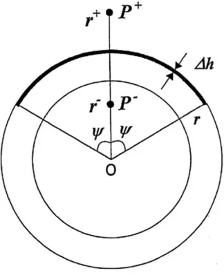
Figure A1 shows a schematic illustration of a thin spher-ical cap of axial symmetry. Lethbe the thickness of the thin spherical cap,ρthe density,ψthe truncation angle, and
t =r/r±the normalized geocentric distance of the spheri-cal cap. Then, the gravity (g±) due to the thin spherical cap at a stationP±on the symmetry axis can be written as
Fig. A1. Schematic illustration of a thin spherical cap with a small thicknesshand a truncation angleψ.rdenotes the radial distance of the spherical cap.P+andP−denote the computation points of gravity at the radial distancesr+andr−, respectively.
(double signs should be taken in the same order; the same as below), where,αis the azimuthal angle andt =h/r±.
Executing the integration of Eq. (A.1) with respect toα andψ, we have
g±=2πGρr± t+t
t
t3−t2cosψ
t2+1−2tcosψ ±t 2 dt.
(A.2) By the Taylor expansion of Eq. (A.2) in the neighbourhood oft =t, and neglecting the higher order terms of more than or equal to (t)2under the condition oft t, Eq. (A.2)
yields
g±≈2πGρH±(t, ψ)h, (h =r±t) (A.3)
(Nozaki, 1999), where,
H±(t, ψ):= t
3−t2cosψ
t2+1−2tcosψ ±t
2. (A.4)
Fig. A2. A graph of the characteristic functionH±(1, ψ)as a function of the truncation angleψwith an argumentt(after Nozaki, 1999). The immediately upper and lower points on the spherical cap correspond tot=1−εandt=1+ε, respectively, whereεis an infinitesimally small positive number. Simplified notationsH+(1, ψ)=H+(1−ε, ψ)andH−(1, ψ)=H−(1+ε, ψ)are used in the text.
Clearly, from Eq. (A.3), H±(t, ψ) defined by Eq. (A.4) is a characteristic function that governs the gravitational behaviour of the spherical cap. A graph of H±(t, ψ) is shown in Fig. A2 as a function of angular distance (or truncation angle)ψwith an argumentt. Especially, whent
takes a limit valuet=1, Eq. (A.4) yields
H±(1, ψ)=
1−cosψ
2 ±1. (A.5)
H±(1, ψ) means H±(1∓ε, ψ), whereε denotes an in-finitesimally small positive number. The first term on the right-hand side of Eq. (A.5) corresponds to the term of sphericity, and the second term does to that of an infinite plate or a Bouguer slab. Whenψ becomes small enough (i.e.ψ ≈0), Eq. (A.3) agrees with gravitational attraction of an infinite plate, i.e. ±2πGρh. On the other hand, when ψ ≈ π, H+(1, ψ) = 2 and Eq. (A.3) becomes 4πGρh on the outer surface of a thin spherical shell of thicknessh. On the inner surface of the spherical shell,
H−(1, ψ) =0 and Eq. (A.3) yield zero. From Eq. (A.5), clearly holds for the following identical equation:
H+(1, ψ)−H−(1, ψ)≡2. (A.6)
This relation can be confirmed on the Fig. A2 that the lines forH+(1−ε, ψ)andH−(1+ε, ψ)are parallel to each other with the distance of 2. Referring to Eq. (A.3), Eq. (A.6) implies that the gravity difference between the immediately upper and lower points on the spherical cap with a small thicknesshis always equal to 4πGρhregardless of the truncation angleψ.
Appendix B.
Differentiation of equations of the generalized Bouguer anomaly with respect to the specific datum levels Hd0,
Hd1andHd2
In this appendix, we demonstrate that the differentiation of Eqs. (29), (30) and (31) in the text with respect to the specific datum levelsHd0,Hd1andHd2results in Eqs. (42),
Here, we shall notice that Eqs. (32), (33) and (33) in the text hold corresponding to every point of horizontal coor-dinates (x,y). Therefore, one can consider the differen-tial quantities in the neighbourhood of(x,y). In this case, it is necessary to differentiate not only gp,Hd0, gp,Hd1, gp,Hd2 and F Abut also Hp andT Cp(1), since they are
functions ofHd0, Hd1 andHd2 that are functions ofxand
y.
Differentiating Eqs. (29), (30) and (31) in the text with respect toHd0,Hd1andHd2, respectively, we have
On the other hand, differentiating Eqs. (14), (16) and (17) in the text with respect to Hd0, Hd1 andHd2, respectively,
Substituing Eqs. (B.4), (B.5) and (B.6) into Eqs. (B.1), (B.2) and (B.3), respectively, and arranging the terms, we have Eqs. (42), (43) and (44) in the text.
Appendix C.
A Note on the Reference Gravity
C.1 A comparison of the Prey-reduced reference gravity field and the normal gravity field
It is stated in an old text book by Garland (1965, p. 50) that an anomaly of gravity is defined by thedifference be-tween the observed (or reduced) gravity at some point and thetheoreticalvalue predicted for the same point. There-fore, for defining the difference of gravity at the geoid, the normal gravity will not be the only onetheoreticalvalue. Other theoretical values are possible. Selection of an appro-priate value depends on the purpose of the anomaly (Gar-land, 1965, p. 59). The Prey-reduced reference gravity field introduced newly in this paper is one of such theoretical
ones, and is not the normal gravity field.
C.2 The normal gravity field (a review) (see Fig. C1)
The normal gravity at the ellipsoid is defined by (Heiska-nen and Moritz, 1967, equation (2-78))
γ =γ0≡γHN0 (C.1)
where the right side termγHN0 is a new notation introduced
here. The normal gravity at the normal heightHN(notation
after Torge, 1989), γN
HN, is defined by the first order
ap-proximation (Heiskanen and Moritz, 1967, equation (8-8), p. 293)
The normal gravity is defined upon and outside the refer-ence ellipsoid, and not inside the referrefer-ence ellipsoid.
C.3 Mass density distribution in the normal gravity field
Outside the reference ellipsoid, the space is free-air, i.e., the mass density is zero. Inside the reference ellipsoid, the mass density distribution does not need to be known (Heiskanen and Moritz, 1967, Sec. 2–7, p. 64). However, the amount of the total mass inside the reference ellipsoid is constant. The simplest mathematical model of such a
Fig. C1. Relation between the Prey-reduced reference gravity field and the normal gravity field. The reference ellipsoid connectsγHRe f