Scalable Coverage Maintenance for Dense Wireless Sensor Networks

(1)

Volume 2007, Article ID 34758,13pages doi:10.1155/2007/34758

Research Article

Scalable Coverage Maintenance for

Dense Wireless Sensor Networks

Jun Lu, Jinsu Wang, and Tatsuya Suda

Bren School of Information and Computer Sciences, University of California, Irvine, CA 92697, USA Received 1 October 2006; Accepted 30 March 2007

Recommended by Mischa Dohler

Owing to numerous potential applications, wireless sensor networks have been attracting significant research effort recently. The critical challenge that wireless sensor networks often face is to sustain long-term operation on limited battery energy. Coverage maintenance schemes can effectively prolong network lifetime by selecting and employing a subset of sensors in the network to provide sufficient sensing coverage over a target region. We envision future wireless sensor networks composed of a vast number of miniaturized sensors in exceedingly high density. Therefore, the key issue of coverage maintenance for future sensor networks is the scalability to sensor deployment density. In this paper, we propose a novel coverage maintenance scheme, scalable coverage maintenance (SCOM), which is scalable to sensor deployment density in terms of communication overhead (i.e., number of trans-mitted and received beacons) and computational complexity (i.e., time and space complexity). In addition, SCOM achieves high energy efficiency and load balancing over different sensors. We have validated our claims through both analysis and simulations.

Copyright © 2007 Jun Lu et al. This is an open access article distributed under the Creative Commons Attribution License, which permits unrestricted use, distribution, and reproduction in any medium, provided the original work is properly cited.

1. INTRODUCTION

The recent advances in microsensor and communication technologies have increased the possibility of manufactur-ing inexpensive small wireless sensors with simple sensmanufactur-ing, processing, and wireless communication capabilities. Lim-ited by their size, small wireless sensors are equipped with a restricted power source and storage capacity. For example,

the typical Crossbow MICA2 mote MPR400CB [1] has a

low-speed 16 MHz microcontroller equipped with only 128 KB flash and 4 KB EEPROM. Powered by two AA batteries, it has the maximal data rate of 38.4 KBaud and a transmission range of about 150 m. Such small wireless sensors are usu-ally deployed in an ad hoc manner to monitor a specified re-gion of interest for various applications such as environment monitoring, target tracking, and distributed data storage.

One fundamental problem faced by current sensor

net-work deployment is eﬃcient provision of the required

cover-age. Specifically, given a target region, how can it guarantee that every point in the region is covered by the required num-ber of sensors, with the object of maximizing the lifetime of the whole network? This problem is challenging due to the limitation of wireless sensor capabilities as well as the ad-hoc deployment properties of wireless sensor networks. One

ef-fective approach to extend sensor network lifetime is to have sensors autonomously schedule their duty cycles according to local information while satisfying global coverage require-ments, which is referred to as coverage maintenance in the literature. We envision future wireless sensor networks com-posed of a vast number of small wireless sensors with very limited processing capability and storage capacity in

exceed-ingly high density [2,3]. Therefore, coverage maintenance

for future wireless sensor networks must be highly scalable to sensor deployment density in terms of communication over-head as well as computational complexity.

In this paper, we propose a novel coverage maintenance scheme, scalable coverage maintenance (SCOM), in which sensors decide their sensing states in a distributive man-ner. SCOM works in two phases—the decision phase and the optimization phase. In the decision phase, sensors start in BOOTSTRAP state, and gradually make their decisions to enter the ACTIVE or INACTIVE state according to lo-cal information on coverage and energy. In the optimization

phase, redundant active sensors turn oﬀwhile still

(2)

redundancy by checking only a small number of locations,

(3) high energy eﬃciency to maintain the required coverage,

and (4) load balancing over sensors.

The rest of this paper is organized as follows.Section 2

specifies SCOM in detail. Theoretical analysis and

simula-tion results are presented in Secsimula-tions3 and4, respectively.

Section 5examines the existing work on sensor network

cov-erage.Section 6concludes the paper.

2. SCALABLE COVERAGE MAINTENANCE (SCOM)

2.1. Assumptions

We assume that sensors are static and each sensor knows its own location. Sensors can acquire the location of neigh-bors through one-hop communication. Such assumptions

are reasonably taken by other researches (e.g., [4–6]) and

supported by the existing workes (e.g., [7–10]). We also

as-sume that sensors have synchronized timers (e.g., [11,12])

and are aware of the amount of their own residual energy. We further assume that communication range of sensors, noted by CR, is at least twice the maximal sensing range, de-noted by SR. This assumption is usually true for real sensors. For example, HMC1002 magnetometer sensors have an SR

of approximately 5 m [13] while MICA2 MPR400CB motes

can transmit about 150 m [1]. Where CR is less than twice

SR, SCOM can work by propagating control beacons through multiple hops.

2.2. Problem statement

Definition 1. A location is covered by a sensor if it is within

the SR of the sensor. A location is said to beK-covered if it is

within the SR of at leastKsensors. A region isK-covered if

every location within the region isK-covered.

Note that according toDefinition 1the sensing perimeter

of a sensor isnotcovered by the sensor.

The number of sensors covering a location is regarded as the coverage degree at that location. The problem is to select

a small number of sensors to maintainK-coverage of the

tar-get region while scheduling others to sleep, which is referred

to as coverage maintenance [14].

Definition 2. Coverage maintenance: given a set of sensorsS

deployed in target regionAand a natural numberK, select

a subsetSofSsuch that

provided bySandS, respectively.

FromDefinition 2, we can see that the subsetS should

provide at leastK-coverage to a location if the location isK

-covered by the full set of sensorsSand should maintain the

original coverage otherwise.

2.3. Scheme description

In SCOM, time is slotted into rounds. At the beginning of each round, each sensor goes through the following two phases.

(1) Decision phase: sensors start in BOOTSTRAP state, and make the decisions to enter the ACTIVE or INACTIVE state according to local information on coverage and energy.

(2) Optimization phase: redundant active sensors turn oﬀ while still guaranteeing the required coverage.

In the decision phase, each sensor is initially in BOOT-STRAP state and has an empty active neighbor list. Before

making its decision, each sensor sets a back-oﬀtimerTdecision

according to its residual energy,

Tdecision=α·(1−p) +, (2)

where p is the residual energy percentage level,αis a

pos-itive real number, and is a small random number

uni-formly distributed within (0,χ].αandχdecide the sensitivity

ofTdecisionto the percentage level of residual energy, that is,

largerαaccentuates while largerχde-emphasizes the diﬀ

er-ence of residual energy among sensors. How to set the

val-ues of αandχis beyond the scope of this paper, and will

be part of our future work. When its timer expires, a sen-sor decides its redundancy by checking whether its sensing

region is K-covered by the sensors in the active neighbor

list, and switches to ACTIVE or INACTIVE state accordingly. Detailed description of the redundancy checking algorithm

is presented in Section 2.4. If a sensor decides to switch to

ACTIVE state, it broadcasts a TURNON beacon including its ID, coordinates, and SR to the neighbors whose sensing re-gions overlap with the sensor. Upon receiving the TURNON beacon, a neighbor in BOOTSTRAP or ACTIVE state adds the sender ID to the active neighbor list and stores the coor-dinates and the SR of the sender. The decision phase lasts for

(α+χ) time units.

After the decision phase, there may exist redundant active sensors because the sensors turning on later may cover the sensing regions of the sensors that had already turned on and create redundancy. To eliminate the redundancy, each active sensor starts the optimization phase right after the decision

phase by setting a back-oﬀtimerToptaccording to its residual

energy,

Topt=α·p+, (3)

whereα,p, andhave the same meaning as in (2). When a

sensor times out, it checks for redundancy based on its active neighbor list and if redundant, switches to INACTIVE state and broadcasts a TURNOFF beacon to its active neighbors. Upon receiving the TURNOFF beacon, an active neighbor removes the sender ID from its active neighbor list. The

op-timization phase also lasts for (α+χ) time units.

In the decision phase, according to (2), sensors with a

(3)

x 8 _i

Figure1: SCOM-redundancy eligibility rule.

back-oﬀperiodTdecisionand thus time out earlier. Therefore,

sensors with a higher percentage level of residual energy have more chance to switch to ACTIVE state. On the other hand,

in the optimization phase, according to (3), sensors with a

higher percentage level of residual energy have a longer

back-oﬀperiodToptand thus time out later. As a result, active

sen-sors with a higher percentage level of residual energy have

less chance to turn oﬀ. In this way, SCOM balances workload

over sensors by employing sensors with more residual energy to provide coverage. It is clear that the precision of time syn-chronization and residual energy estimation may impact the

performance of load balancing, but has no eﬀect on

guaran-teeing required coverage.

2.4. Redundancy eligibility rule

The key operation of SCOM is to decide a sensor’s redun-dancy given the location of the neighbors in the active neigh-bor list. Obviously, a sensor is redundant if its sensing region

isK-covered by its neighbors. Here we propose a redundancy

eligibility rule, by which a sensor is able to decide whether its

sensing region isK-covered by its neighbors simply by

check-ing the coverage at a few locations within its senscheck-ing region.

We first assume thatnotwo sensors are at the same

loca-tion, and later extend the proposed eligibility rule to handle multiple sensors at the same location. We describe redun-dancy eligibility rules for two cases: homogeneous SR (i.e., sensors have the same SR) and heterogeneous SR (i.e.,

sen-sors may have diﬀerent SRs).

2.4.1. Sensors with homogeneous SR

For clarity, we have defined a sensor’s critical point set.

Definition 3. Critical point set-sensori’s critical point setSi

contains, for each neighborn, (1) the intersection points

be-tween the sensing perimeters ofnand other neighbors within

the sensing region of sensori, or if such intersection points

donotexist, (2) one intersection point between the sensing

perimeters ofnand sensori.

For example, inFigure 1(a),Sicontains three intersection

points between sensori’s neighbors (i.e.,x,yandz) and one

intersection point between a neighbor and sensori(i.e.,v).

Note that two tangent sensing perimeters are regarded to in-tersect each other at the point of contact.

Theorem 1. In a homogeneous sensor network, given a natural numberK, (1) ifSiis not empty, the sensing region of sensori isK-covered by its neighbors if and only if each critical point in SiisK-covered by its neighbors; (2) ifSiis empty, the sensing region of sensoriis notK-covered by its neighbors.

Proof. (1) WhenSiis not empty, the sensing region of

sen-sor i is divided into subregions by the sensing perimeters

of neighbors. For example, in Figure 1(a), sensor i’s

sens-ing region is divided into eight sub-regions. Since a sen-sor’s sensing perimeter is not covered by the sensor itself

ac-cording to Definition 1, the coverage of a sub-region is

al-ways higher than or equal to the coverage of adjacent

criti-cal points. For example, inFigure 1(a), the coverage of

sub-region 8 is higher than or equal to the coverage of adjacent

critical pointx,yandz. Thus, the minimal coverage of

sub-regions isno less thanthe minimal coverage of critical points.

On the other hand, for each critical point, we can always find an adjacent sub-region with the same coverage. For example, inFigure 1(a), critical pointsx,y, andzhave the same cover-age as subregions 2, 5, and 7, respectively. Thus, the minimal

coverage of critical points isno less thanthe minimal

cover-age of sub-regions. Therefore, the minimal covercover-age of criti-cal points equals the minimal coverage of sub-regions, which

means that if each critical point inSiisK-covered by sensor

i’s neighbors, the sensing region of sensoriisK-covered by

its neighbors, and vice versa. (2) An emptySiimplies that the

sensing regions of sensoriand its neighbors do not overlap.

Thus, the sensing region of sensoriis notK-covered by its

(4)

x i

y

SRi

Figure2:Theorem 1cannot be applied for heterogeneous sensors.

2.4.2. Sensors with heterogeneous SR

When sensors have diﬀerent SRs,Theorem 1may not hold.

For example, inFigure 2,Sicontains critical pointsxandy,

both of which are 1-covered by sensor i’s neighbors.

How-ever, the sensing region of sensor iis not 1-covered by its

neighbors. To accommodate heterogeneous sensors, we have defined extended critical point set.

Definition 4. Extended critical point set-sensori’s extended

critical point setESi contains (1) the critical points in

crit-ical point setSi, and (2) a sampling point on each sensing

perimeter that is within sensori’s sensing region and does

notintersect with any other sensing perimeter.

For example, in Figure 1(b), Si contains three critical

points,x,yandz. There are two sensing perimeters that are

contained in sensori’s sensing region and that do not

inter-sect with other sensing perimeters. Thus,ESialso containsv

andwas the sampling points on the two sensing perimeters.

Therefore,ESicontains five critical points,x,y,z,w, andv.

Theorem 2. In a heterogeneous sensor network, given a

nat-ural numberK, (1) ifESi is not empty, the sensing region of sensoriisK-covered by its neighbors if and only if each critical point inESiisK-covered by its neighbors; (2) ifESiis empty, the sensing region of sensoriisK-covered by neighboring sen-sors if and only if a sampling point within the sensing region of sensoriisK-covered by its neighbors.

Proof. (1) The proof is similar toTheorem 1. We can prove

that the minimal coverage of the critical points inESiis equal

to the minimal coverage of the sub-regions, which means

that if each critical point inESi is K-covered by sensori’s

neighbors, the sensing region of sensor iis alsoK-covered

by its neighbors, and vice versa. (2) When sensors have het-erogeneous SR, an empty extended critical point set does not necessarily mean that the sensing region has no overlap with

others. For example, inFigure 1(b),ESncontains no critical

point, but sensorn’s sensing region is contained in the

sens-ing regions of its neighbors. In this case, the senssens-ing region of

nisnotdivided into sub-regions. Thus, sensorncan decide

whether its sensing region isK-covered by checking the

cov-erage of any sampling point within its sensing region.

x

v i

y _z

u

Figure3: Critical point set versus the existing algorithms.

For the description above, we assume that no two sensors are at the same location. The redundancy eligibility rules

de-scribed in Theorems1and2can be easily extended to

accom-modate the special case of multiple sensors at the same

loca-tion. For sensors with homogeneous SR, ifSiis not empty,

the coverage of the critical pointson sensori’s sensing

perime-ter(e.g.,vinFigure 1(a)) is increased by the number of

sen-sors at the same location as sensori; ifSiis empty, the

sens-ing area of sensoriis covered by the number of sensors at the

same location as sensori. In the case of heterogeneous SR, if

ESiis not empty, the coverage of the critical pointson sensor

i’s sensing perimeter(e.g.,zinFigure 1(b)) is increased by the number of sensors at the same location and with the same SR

as sensori; in the case of an emptyESi, we can still decide the

redundancy of sensoriby checking a sampling point within

its sensing region.

We note that a similar idea was proposed in Hall (1998)

[15, page 56] to study the problem of covering a sphere with

circular caps and later developed by [16,17] forK-coverage

maintenance in sensor networks. In their algorithms, how-ever, the set of points to be checked by each sensor includes all the intersection points between the sensing perimeters of any two neighbors or between a neighbor and the sen-sor itself. Thus, their algorithms are required to check more points, and as a result, incur more computation overhead.

For example, inFigure 3, critical point setSi only contains

pointx, while the existing algorithms are required to

com-pute coverage at all the intersection points, x, y,z,u, and

v. Furthermore, the algorithms proposed in [15–17], assume

homogeneous caps or sensors and cannot be applied to het-erogeneous sensors.

3. SCHEME ANALYSIS

In this section, we analyze and compare the scalability of

SCOM with the existing schemes proposed in [4,6].

In the scheme proposed in [4] (hereinafter referred to as

thesponsored sector (SS) scheme), every sensor calculates its

eligibility to turn oﬀ. A sensor is eligible to turn oﬀif its

sens-ing region is contained by the union of the sponsored sectors

oﬀered by its active neighbors within SR. A back-oﬀ

mecha-nism is used to avoid blind points caused by simultaneous

decisions of multiple sensors. After the back-oﬀ period, a

(5)

to the neighbors within SR. Upon receiving the TURNOFF beacon, every neighbor removes the sensor from the neigh-bor list so that the sensor will not be counted to decide the eligibility of other sensors.

In the scheme proposed in [6] (referred to as thebasic

dif-ferentiated surveillance (DS)), each sensor randomly gener-ates a time-reference point and broadcasts it to the neighbors within twice SR. The target region is covered with a virtual square grid. A sensor decides the working schedule for each grid point within the SR based on its own time-reference point and the time-reference points of the neighbors cov-ering the grid point. The final schedule of the sensor is the union of the working schedules for all the grid points. The fi-nal schedule can be optimized through exchanging schedule information among neighboring sensors (referred to as 2nd pass diﬀerentiated surveillance (DS)).

Let us investigate a sensor network composed ofN

ho-mogeneous sensors with sensing rangeRuniformly deployed

in a square area of×(R). For each scheme, we

exam-ine the growth of communication overhead (i.e., the num-ber of transmitted and received beacons) and computational

complexity (i.e., space and time complexity) asN→ ∞.

3.1. SCOM

Assume that there areMsensors turning on in the decision

phase andN(NM) active sensors in the final network.

Theorem 3. Given a limited required degree of coverageK, one has

lim

N→∞E(M)=O(1), (4)

whereE(M)is the expected number of sensors that turn on in the decision phase of SCOM.

Proof. Without losing generality, we investigate a sensor

net-work within a unit square area (i.e.,is set to 1).

Let us first consider the independent turning on process,

in whichNsensors are uniformly deployed in BOOTSTRAP

state initially and then randomly and independently turn on one by one until 1-coverage is fulfilled. It is clear that the location of the sensors turning on follows a stationary two-dimensional Poisson point process. Denote the density of the Poisson point process and the vacancy (i.e., the region not

1-covered) asλandVλ, respectively. It has been shown in Hall

(1988) [15, Theorem 3.11, page 180] that

0.05ζλ< P

Obviously, the (n+ 1)th sensor turns on only when then

sensors that are already on cannot cover the area. Thus, the

probability of requiring more thannactive sensors can be

calculated as the probability of vacancy larger than 0 withn

active sensors, or

We can easily prove the convergence of the series in (7)

with the ratio test

lim

The convergence of the series indicates thatE(M) to

pro-vide 1-coverage is bounded by an upper limit, or O(1) as

N→ ∞.

In [18] (the proof ofTheorem 1), Zhang and Huo

pre-sented an upper bound of the probability that a region isnot

K-covered. With the upper bound, we can prove that the

ex-pected number of sensors to provideK-coverage is also

up-per bounded by a limit, orO(1) asN→ ∞. Since the proof is

essentially the same as the 1-coverage case, we have omitted it here.

We have shown thatE(M) of the independent turning on

process isO(1) asN → ∞. The diﬀerence between the

de-cision phase of SCOM and the independent turning on pro-cess is that, in the decision phase of SCOM, a sensor turns on only when it is not redundant (instead of turning on inde-pendently). It is clear that the decision phase of SCOM yields fewer active sensors than the independent turning on

pro-cess. Therefore,E(M) of the decision phase of SCOM is also

O(1) asN→ ∞.

3.1.1. Communication overhead

(a) Number of transmitted beacons

In SCOM, sensors transmit TURNON beacons and TURNOFF beacons in the decision phase and optimization

phase, respectively. It is clear that sensors transmit M

TURNON beacons in the decision phase and (M −N)

TURNOFF beacons in the optimization phase (note thatN

is the number of active sensors after the optimization phase,

which is no larger thanM). The total number of transmitted

beacons is (2M−N), orO(1) asN→ ∞.

(b) Number of received beacons

(6)

state of each sensor is upper bounded by Nπ(2R)2_/2 _(in

SCOM neighbor sensors are within the range of 2R). Since

there are in totalMTURNON beacons transmitted, the total

number of TURNON beacons received is upper bounded by

MNπ(2R)2_/2_{. In the optimization phase, only the sensors in}

ACTIVE state accept TURNOFF beacons. Since the average number of neighbors in ACTIVE state of each sensor is upper

bounded byMπ(2R)2_/2_{and there are (}_M₋_N_{) TURNOFF}

beacons transmitted, the total number of TURNOFF beacons

received is upper bounded byMπ(2R)2₍_M₋_N₎_/2_{. The}

to-tal number of TURNON and TURNOFF beacons received is

upper bounded byMNπ(2R)2_/2₊_Mπ₍₂_R₎2₍_M₋_N₎_/2_{, or}

O(N) asN→ ∞.

3.1.2. Computational complexity

(a) Time complexity

In the decision phase, each sensor applies the redundancy eli-gibility rule to decide redundancy. The critical point set com-prises the intersection points between the sensing perime-ters of the sensor and its active neighbors. The average num-ber of active neighbors of each sensor is upper bounded by

Mπ(2R)2_/2_{. Thus, the number of critical points is upper}

bounded by 2·(Mπ(2R)2_/2_{)(1 +}_Mπ₍₂_R₎2_/2_{). For each}

critical point, a sensor needs to check for each active neigh-bor whether the critical point is covered. Thus, the num-ber of basic computation steps to decide the redundancy is

2·(Mπ(2R)2_/2₎2_{(1 +}_Mπ₍₂_R₎2_/2_{), or}_O_{(1) as}_N _{→ ∞}_{. In}

the optimization phase, each active sensor checks its redun-dancy once, the number of basic computation steps of which

is alsoO(1). Thus, the time complexity isO(1) asN→ ∞.

(b) Space complexity

The memory size required for each sensor to execute SCOM

is mainly composed of (1)Mπ(2R)2_/2_{entries for neighbors}

in ACTIVE state and (2) 2·(Mπ(2R)2_/2_{)(1 +}_Mπ₍₂_R₎2_/2₎

entries for critical points. Thus, the space complexity isO(1)

asN→ ∞.

3.2. Sponsored sector scheme

Denote the number of active sensors in the resulting network

of SS asN. Similarly, we can derive thatE(N) of SS isO(1)

whenN→ ∞.

Each sensor to turn oﬀsends a TURNOFF beacon to inform

its neighbors. Obviously, the total number of TURNOFF

beacons transmitted is (N−N), orO(N) asN→ ∞.

Only sensors that have not made their decisions need to

re-ceive TURNOFF beacons. In the best case, all the N

ac-tive sensors make decisions before the other sensors, and

thus no beacon is received by theseN sensors. Therefore,

TURNOFF beacons are only exchanged among the (N−N)

sensors. For the ith sensor to turn oﬀ, the average

num-ber of received TURNOFF beacons is (i−1)πR2_/2 _{(in SS}

neighbor sensors are within the range ofR). Thus, the total

number of TURNOFF beacons received by all the sensors is N−N

i=1 ((i−1)πR2/2), orO(N2) asN→ ∞.

In SS, each sensor checks all the active neighbors to de-cide its redundancy. Thus, the computational complexity is in the order of the number of active neighbors. A lower bound of the computational complexity can be derived by

merely counting the computation overhead of the (N−N)

inactive sensors in the resulting network. For the ith

sen-sor to turn oﬀ, the average number of active neighbors is

(N−i+ 1)(πR2_/2_{). Thus, the total computational}

complex-ity of all the sensors is O(iN=−1N((N −i+ 1)πR2/2)), or

O(N2_{). Thus, the average time complexity}_{per sensor}_is_O₍_N₎

asN→ ∞.

The memory size required for each sensor is mainly

com-posed ofNπR2_/2_{entries on average to store neighbor states.}

Thus, the space complexity isO(N).

3.3. Basic differentiated surveillance

It is noted in [6] that the time-reference point beacons can be

combined with the beacons to exchange coordinates among neighbors. Thus, there is no extra communication overhead in Basic DS.

As described in [6], there are averagelyπR2_/d2 _{grid points}

within a sensor’s sensing region, where d is the unit grid

size. Each sensor decides the schedule for each grid point

ac-cording to neighbors’ time reference points. GivenNπR2_/2

neighbors on average covering the same grid point, it takes

(NπR2_/2_{) log(}_NπR2_/2_{) basic computation steps to sort}

time-reference points and another constant timeCto decide

the sensor’s schedule for the grid point. Finally, the sched-ules for all the grid points are combined to generate the

in-tegrated schedule for the sensor, which costs 2πR2_/d2 _basic

computation steps. Thus, the overall computational

com-plexity is (πR2_/d2₎₍₍_NπR2_/2_{) log(}_NπR2_/2_{) +}_C_{) + 2}_πR2_/d2_,

(7)

As described in [6], the memory size required for each

sen-sor is mainly composed of (1)Nπ(2R)2_/2_{entries on average}

for a neighbor table, (2)NπR2_/2_{memory units on average}

for sorting time reference points and (3) 2πR2_/d2 _memory

units for schedules of grid points. The total space complexity

isO(N).

3.4. 2nd pass differentiated surveillance

In 2nd pass DS, each sensor sends two beacons to inform its original integrated schedule and optimized schedule to neighbors. Thus, the total number of beacons transmitted is O(N).

First, each sensor receives the beacons for original integrated schedules from its neighbors. The total number of received

beacons isN·(Nπ(2R)2_/2_{), or}_O₍_N2_{). Second, only sensors}

that have not optimized need to receive the beacons for

opti-mized schedules. For theith sensor to optimize, the average

number of the received beacons is (i−1)π(2R)2_/2_{. Thus, the}

total number of received beacons for the optimized

sched-ule isNi=1((i−1)π(2R)2/2), orO(N2). Therefore, the total

number of received beacons isO(N2_).

In 2nd pass DS, each sensor carries out the basic DS algo-rithm and optimizes its schedule according to the schedules

of its neighbors, both of which can be done inO(NlogN).

Thus, the time complexity isO(NlogN).

The memory capacity required for each sensor is mainly

composed of (1)Nπ(2R)2_/2_{entries on average for a}

neigh-bor table, (2) NπR2_/2 _{memory units on average for}

sort-ing time reference points on average, (3) 2πR2_/d2 _memory

units on average for schedules for all the grid points and

(4)Nπ(2R)2_/2 _{entries on average for integrated schedules}

of neighboring sensors. Thus, the space complexity isO(N).

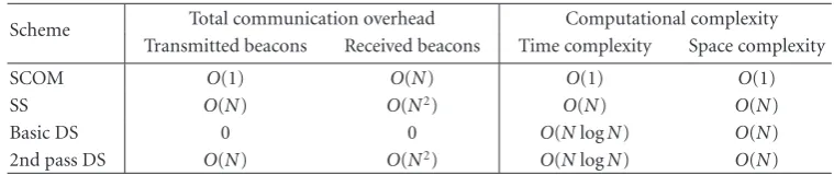
Table 1summarizes the scalability of diﬀerent coverage maintenance schemes to sensor deployment density (note

that given a fixed , N actually represents sensor

deploy-ment density) in terms of total communication overhead (i.e., number of transmitted and received beacons) and com-putational complexity (i.e., time and space complexity). We can see that SCOM outperforms other schemes except for the communication overhead of basic DS. However, the

achieve-ment of Basic DS is at the cost of energy eﬃciency and

adapt-ability to sensor network dynamics such as sensor failures.

An integrated schedule generated by basic DS is a super set of schedules for many grid points, and therefore may be more

than suﬃcient to provide the coverage guarantee. Moreover,

when executed in multiple rounds, basic DS is not able to restore coverage from sensor failure because sensors are un-aware of the failure of neighboring sensors. Although it is possible to use heartbeat signals to check the state of

neigh-bors as described in [6], the communication overhead to

transmit and receive heartbeat signals isO(N) andO(N2_),

re-spectively. In contrast, at the beginning of each round, since only working sensors turn on and transmit TURNON bea-cons, SCOM can easily restore the coverage by substituting failed sensors with working ones.

Note that we assumed sensors with homogeneous SR in the above analysis. The analysis results are also valid for het-erogeneous sensor networks as long as the SR is within a lim-ited range.

From the above analysis, we know that SCOM is scal-able because it only turns on necessary sensors in the deci-sion phase. We have shown that, given the required degree of coverage, the number of sensors turning on in the deci-sion phase is a limited value as sensor deployment density approaches infinity. Since each sensor only communicates to its active neighbors and only considers the active neighbors to make its decision, the communication and computation overhead per sensor remains limited with the increase of sen-sor deployment density. A similar technique is adopted by

[17,19,20], but they do not provide specific analysis and

evaluation of scalability of their schemes.

In summary, communication overhead and

computa-tional complexityper sensorare limited as the sensor

deploy-ment density approaches infinity, which makes SCOM favor-able for dense sensor networks composed of simple sensors equipped with a slow processor and small storage.

4. SIMULATION STUDY

In this section, we compare the performance of SCOM with SS, DS, and 2nd pass DS schemes through simulations.

4.1. Simulation setup

The simulations are carried out over a square region of

100 m×100 m with wrap around in both dimensions. Thus,

the results are representative of an infinite system, and there-fore apply to typical large-scale sensor networks. Sensors are uniformly deployed in the square region.

In SCOM,αandχof (2) and (3) are set to 10.0 and 1.0,

respectively. We simulated both homogeneous and hetero-geneous sensor networks. For homohetero-geneous networks, SR is fixed at 10 m. For heterogeneous networks, a sensor’s SR is uniformly chosen from three possible values: 5 m, 10 m, and 15 m.

4.2. Simulation results

The simulation results are shown for communication

over-head, computational complexity, energy eﬃciency, and load

(8)

Table1: Communication overhead and computational complexity.

Scheme Total communication overhead Computational complexity Transmitted beacons Received beacons Time complexity Space complexity

SCOM O(1) O(N) O(1) O(1)

SS O(N) O(N2₎ _O₍_N₎ _O₍_N₎

Basic DS 0 0 O(NlogN) O(N)

2nd pass DS O(N) O(N2₎ _O₍_N_log_N₎ _O₍_N₎

Figures 4and5show the communication overhead of

dif-ferent schemes to provide 1-coverage for sensor networks with homogeneous SR and heterogeneous SR, respectively.

Figure 4 illustrates the total number of beacons transmit-ted and received in homogeneous sensor networks. Basic DS is not shown because it incurs no extra communica-tion overhead by piggybacking the beacons to exchange time-reference points to the location exchanging beacons (as

shown inTable 1, the number of transmitted and received

beacons of basic DS is 0).Figure 4(a)depicts the total

num-ber of transmitted beacons with various sensor deployment densities. We can observe that the number of transmitted beacons of SCOM remains stable while that of the other two schemes grows linearly with the increase of sensor deploy-ment density. We also see that the growth rate of SS is lower than that of 2nd pass DS because in SS only redundant sen-sors need to send beacons while every sensor transmits two beacons in 2nd pass DS. The simulation results confirm the

analysis results inTable 1.Figure 4(b)shows that the

num-ber of received beacons of SCOM increases linearly with sen-sor deployment density, while that of 2nd pass DS grows quadratically. More detailed analysis reveals that the growth rate of SS is also quadratic, although much lower than 2nd

pass DS. This observation also agrees withTable 1.Figure 5

describes the number of transmitted and received beacons in heterogeneous sensor networks. Our observations are similar toFigure 4; SCOM is more scalable than SS and 2nd pass DS in terms of communication overhead.

The analysis inSection 3reveals that the computational

com-plexity is decided by the number of neighbors. Thus, we use the average number of neighbors of each sensor to mea-sure the computational complexity. The results are shown in

Figure 6for 1-coverage. Since the average numbers of neigh-bors in the two phases (i.e., the decision phase and

opti-mization phase) of SCOM are diﬀerent, we show the

av-erage number of active neighbors in both phases. Because 2nd pass DS always has more computation overhead than

Basic DS, we only show the results of basic DS.Figure 6(a)

depicts the average number of active neighbors in homoge-neous networks. We can see that the average number of ac-tive neighbors of both phases of SCOM remains constant, whereas that of SS and basic DS rises linearly with the growth

of sensor deployment density, which means that the com-putation overhead per sensor of SCOM remains stable (i.e.,

O(1)) while that of SS and basic DS increases with network

deployment density. We also see that SS has fewer neighbors than basic DS because SS only considers neighbors within the range of SR. Again, this observation conforms to the

analy-sis results inTable 1. As shown inFigure 6(b), we obtained

similar results for heterogeneous sensor networks.

4.2.3. Energy efficiency

Figure 7 illustrates the energy consumption of monitoring to provide coverage for homogeneous sensor networks. The energy consumption is measured in units, which means the amount of energy consumed by an active sensor for a unit of

time. In [21], a theoretical lower bound of the active sensor

density to achieve 1-coverage is provided as 2/√27SR2, and

is calculated inFigure 7(a)as a baseline for comparison. We

can see that SCOM consumes less energy than the other three schemes. For example, the energy consumption of SCOM is about 16% less than that of 2nd Pass DS, which is the best among the other schemes. This is because SCOM uses ac-tual SR while DS schemes use smaller conservative SR in

or-der to avoid small sensing holes. FromFigure 7(a), we also

observe that SCOM consumes about 75% more energy than

the theoretical lower bound.Figure 7(b)illustrates the

en-ergy consumption to provide diﬀerentiated degree of

cover-age (i.e.,K-coverage), for which the sensor deployment

den-sity is fixed at 8 sensors/SR2_{. Since [}₆_{] does not specify how}

to use 2nd pass DS to provideK-coverage, 2nd pass DS is

not shown. We can see that SCOM significantly outperforms both basic DS and SS. The large discrepancy between SCOM and basic DS is due to the fact that a sensor’s integrated schedule generated by basic DS is a super set of its schedules

for many grid points, and therefore is more than suﬃcient

to provide the coverage guarantee. Moreover, we notice that, with the increase of the required degree of coverage, the en-ergy consumption of SCOM grows slower than that of basic DS and SS, and only slightly faster than the theoretical lower

bound. The energy eﬃciency of diﬀerent schemes in

hetero-geneous sensor networks is shown inFigure 8. Again, SCOM

conserves more energy than other schemes.

4.2.4. Load balancing

As described in Section 2.3, by setting the back-oﬀtimers

(9)

500

Sensor deployment density (number of sensors/SR2₎ SCOM

SS 2nd pass DS

(b) Beacons received

Figure4: Communication overhead (1-coverage, homogeneous SR=10 m).

500

SS 2nd pass DS

(b) Beacons received

Figure5: Communication overhead (1-coverage, heterogeneous SR=5/10/15 m).

load balancing by employing sensors with more percent-age of residual energy to provide network coverpercent-age. Here we compare SCOM with a modified version of SCOM

(re-ferred to asSCOM without load balancing). In SCOM

with-out load balancing, instead of setting timers according to the

amount of residual energy using (2) and (3), sensors simply

adopt random back-oﬀtimers. In the simulations, each

sen-sor starts with 100% energy and the energy consumption rate

is fixed at 10% per round.Figure 9(a)depicts the network

(10)

0

Sensor deployment density (number of sensors/SR2₎ SCOM-decision phase

SCOM-optimization phase

SS Basic DS (b) Heterogeneous SR=5/10/15 m

Figure6: Average number of active neighbors (1-coverage).

50

The required degree of coverage (K) SCOM

SS

Basic DS

Theoretical lower bound (b) Sensor deployment density=8 sensors/SR2

Figure7: Energy eﬃciency (homogeneous SR=10 m).

considerably extends the lifetime of networks. Figure 9(b)

provides a closer look at the load balancing of SCOM by showing how the standard deviation of residual energy in a network of 800 sensors evolves. We can see that SCOM low-ers the residual energy deviation significantly, which means

that SCOM better distributes workload among diﬀerent

sen-sors.

The simulation results presented above confirm that SCOM is highly scalable in terms of communication

over-head and computational complexity, while remaining eﬀ

ec-tive to conserve energy and balance load among sensors.

5. RELATED WORK

(11)

20

The required degree of coverage (K) SCOM

SS Basic DS

(b) Sensor deployment density=8 sensors/SR2

Figure8: Energy eﬃciency (heterogeneous SR=5/10/15 m).

30

SCOM without load balancing (a)

SCOM without load balancing (b)

Figure9: SCOM load balancing (1-coverage).

Some of the research studies investigate sensor network coverage from a theoretical perspective. For example, Zhang

and Huo [18] derived the asymptotic upper bound of the

1-lifetime (i.e., the network 1-lifetime to provide full coverage)

for an infinite monitored area and the upper bound of theα

-lifetime (i.e., the network -lifetime to provideα-portion

cov-erage) for a finite monitoring area. The authors of [22]

ana-lyzed sensor network coverage of wireless sensor networks by studying the relation between the number of neighbors and

the coverage redundancy. Liu and Towsley [23] investigated

the limits of sensor network coverage using diﬀerent coverage

measures, that is, area coverage, node coverage fraction and detectability. The critical conditions of sensor network

con-figuration for asymptotic coverage are investigated in [24].

There are many coverage maintenance schemes

pro-posed. For example, Tian and Georganas [4] presented a

node scheduling algorithm to turn oﬀsensors whose

(12)

range. Randomized as well as coordinated sleep algorithms

were proposed in [25] to maintain network coverage using

low duty-cycle sensors. The randomized algorithm enables each sensor to independently sleep under a certain proba-bility, while the coordinated sleep algorithm allows a sen-sor to enter sleep state if its sensing area is fully contained by the union set of its neighbors. An algorithm was

pro-posed in [5] to decide the coverage of a target area by merely

checking the coverage state of sensing perimeters. Yan et

al. [6] proposed an adaptable energy-eﬃcient sensing

cov-erage protocol, in which each sensor broadcasts a random time-reference point, and decides its duty schedule based on

neighbors’ time-reference points. Co-Grid proposed in [14]

schedules sensors by adopting a distributed detection model based on data fusion. Abrams et al. studied a variant of the

NP-hard SET K-COVER problem in [26], partitioning the

sensors intoKcovers such that as many areas are monitored

as frequently as possible. Xing et al. [16] studied the

relation-ship between coverage and connectivity, and proposed a cov-erage maintenance scheme, covcov-erage configuration protocol (CCP), which, when integrated with an existing connectivity maintenance scheme, is able to provide both coverage and

connectivity guarantees. In [27], Kumar et al. proposed

al-gorithms to decide quickly whether a deployed region isK

-barrier covered. Two notions of probabilistic -barrier cover-age, the weak and strong barrier covercover-age, are introduced and

studied. Cardei et al. [28] proposed an eﬃcient scheme to

cover a set of targets with known locations in a randomly and densely deployed sensor network. The target coverage prob-lem is modeled as the maximal set cover probprob-lem and two

heuristics are proposed and evaluated. Zhang and Huo [19]

presented a scheme to optimize coverage maintenance while providing global connectivity by keeping a minimum num-ber of active sensors to minimize coverage redundancy.

6. CONCLUSION

In this paper, we introduced SCOM that conserves energy while preserving the required sensing coverage by allowing sensors to autonomously decide their active/inactive states. An important property of SCOM is the high scalability to sensor deployment density in terms of communication over-head and computational complexity, which makes SCOM suitable for densely deployed sensor networks composed of simple sensors. We showed that the scalability of SCOM is better than the earlier works through both theoretical analysis and simulation study. Moreover, we demonstrated through simulation study that SCOM outperforms several

existing competitors on energy eﬃciency and eﬀectively

bal-ances workload among sensors.

ACKNOWLEDGMENTS

This research is supported by the NSF through Grants ANI-0083074, ANI-9903427, and ANI-0508506, by DARPA through Grant MDA972-99-1-0007, by AFOSR through Grant MURI F49620-00-1- 0330, and by grants from the Cal-ifornia MICRO and CoRe programs, Hitachi, Hitachi

Amer-ica, Hitachi CRL, Hitachi SDL, DENSO IT Laboratory, NICT (National Institute of Communication Technology, Japan), Nippon Telegraph and Telephone (NTT), NTT Docomo, NS Solutions Corporation, Fujitsu and Novell.

REFERENCES

[1] Crossbow Technology Inc., MICA2 Data Sheet, http:// www.xbow.com/products/Product pdf files/Wireless pdf/ MICA2 Datasheet.pdf.

[2] K. S. J. Pister, J. M. Kahn, and B. E. Boser, “Smart Dust: Wireless Networks of Millimeter-Scale Sensor Nodes,” High-light Article in 1999 Electronics Research Laboratory Research Summary, 1999.

[3] B. Warneke, M. Last, B. Liebowitz, and K. S. J. Pister, “Smart dust: communicating with a cubic-millimeter computer,” Computer, vol. 34, no. 1, pp. 44–51, 2001.

[4] D. Tian and N. D. Georganas, “A coverage-preserving node scheduling scheme for large wireless sensor networks,” in Pro-ceedings of the 1st ACM International Workshop on Wireless Sensor Networks and Applications (WSNA ’02), pp. 32–41, At-lanta, Ga, USA, September 2002.

[5] C.-F. Huang and Y.-C. Tseng, “The coverage problem in a wire-less sensor network,” inProceedings of the 2nd ACM Interna-tional Workshop on Wireless Sensor Networks and Applications (WSNA ’03), pp. 115–121, San Diego, Calif, USA, September 2003.

[6] T. Yan, T. He, and J. A. Stankovic, “Diﬀerentiated surveil-lance for sensor networks,” inProceedings of the 1st Interna-tional Conference on Embedded Networked Sensor Systems (Sen-Sys ’03), pp. 51–62, Los Angeles, Calif, USA, November 2003. [7] J. Albowicz, A. Chen, and L. Zhang, “Recursive position

es-timation in sensor networks,” inProceedings of International Conference on Network Protocols (ICNP ’01), pp. 35–41, River-side, Calif, USA, November 2001.

[8] N. Bulusu, J. Heidemann, and D. Estrin, “GPS-less low-cost outdoor localization for very small devices,” IEEE Personal Communications, vol. 7, no. 5, pp. 28–34, 2000.

[9] P. Bahl and V. N. Padmanabhan, “RADAR: an in-building RF-based user location and tracking system,” inProceedings of the 19th Annual Joint Conference of the IEEE Computer and Com-munications Societies (INFOCOM ’00), vol. 2, pp. 775–784, Tel Aviv, Israel, March 2000.

[10] N. B. Priyantha, A. Chakraborty, and H. Balakrishnan, “The Cricket location-support system,” inProceedings of the 6th An-nual International Conference on Mobile Computing and Net-working (MOBICOM ’00), pp. 32–43, Boston, Mass, USA, August 2000.

[11] H. Dai and R. Han, “TSync: a lightweight bidirectional time synchronization service for wireless sensor networks,”ACM SIGMOBILE Mobile Computing and Communications Review, vol. 8, no. 1, pp. 125–139, 2004.

[12] J. Elson, L. Girod, and D. Estrin, “Fine-grained network time synchronization using reference broadcasts,” inProceedings of the 5th Symposium on Operating System Design and Implemen-tation (OSDI ’02), pp. 147–163, Boston, Mass, USA, December 2002.

[13] Crossbow Technology Inc.,MTS/MDA Sensor and Data Ac-quisition Boards Users Manual, Crossbow Technology Inc, San Jose, Calif, USA, 2003.

(13)

on Information Processing in Sensor Networks (IPSN ’04), pp. 414–423, Berkeley, Calif, USA, April 2004.

[15] P. Hall,Introduction to the Theory of Coverage Processes, John Wiley & Sons, New York, NY, USA, 1988.

[16] G. Xing, X. Wang, Y. Zhang, C. Lu, R. Pless, and C. Gill, “In-tegrated coverage and connectivity configuration for energy conservation in sensor networks,”ACM Transactions on Sen-sor Networks, vol. 1, no. 1, pp. 36–72, 2005.

[17] A. Gallais, J. Carle, D. Simplot-Ryl, and I. Stojmenovi´c, “Local-ized sensor area coverage with low communication overhead,” inProceedings of the 4th Annual IEEE International Conference on Pervasive Computing and Communications (PerCom ’06), pp. 328–337, Pisa, Italy, March 2006.

[18] H. Zhang and J. C. Hou, “On deriving the upper bound ofα -lifetime for large sensor networks,” inProceedings of the 5th ACM International Symposium on Mobile Ad Hoc Network-ing and ComputNetwork-ing (MobiHoc ’04), pp. 121–132, Tokyo, Japan, May 2004.

[19] H. Zhang and J. C. Huo, “Maintaining sensing coverage and connectivity in large sensor networks,”Ad Hoc & Sensor Wire-less Networks, vol. 1, no. 1-2, pp. 89–123, 2005.

[20] J. Lu and T. Suda, “Coverage-aware self-coordination in sen-sor networks,” Tech. Rep. 04-19, School of Information and Computer Sciences, UC Irvine, Irvine, Calif, USA, 2004. [21] F. Ye, G. Zhong, S. Lu, and L. Zhang, “Energy eﬃcient robust

sensing coverage in large sensor networks,” Tech. Rep., UC Los Angeles, Los Angeles, Calif, USA, 2002.

[22] Y. Gao, K. Wu, and F. Li, “Analysis on the redundancy of wire-less sensor networks,” inProceedings of the 2nd ACM Interna-tional Workshop on Wireless Sensor Networks and Applications (WSNA ’03), pp. 108–114, San Diego, Calif, USA, September 2003.

[23] B. Liu and D. Towsley, “A study of the coverage of large-scale sensor networks,” inProceedings of IEEE International Conference on Mobile Ad-Hoc and Sensor Systems (MASS ’04), pp. 475–483, Fort Lauderdale, Fla, USA, October 2004. [24] S. Kumar, T. H. Lai, and J. Balogh, “On K-coverage in a mostly

sleeping sensor network,” inProceedings of the 10th Annual International Conference on Mobile Computing and Network-ing (MOBICOM ’04), pp. 144–158, Philadelphia, Pa, USA, September-October 2004.

[25] C.-F. Hsin and M. Liu, “Network coverage using low duty-cycled sensors: random & coordinated sleep algorithms,” in Proceedings of the 3rd International Symposium on Information Processing in Sensor Networks (IPSN ’04), pp. 433–442, Berke-ley, Calif, USA, April 2004.

[26] Z. Abrams, A. Goel, and S. Plotkin, “Set K-cover algorithms for energy eﬃcient monitoring in wireless sensor networks,” in Proceedings of the 3rd International Symposium on Information Processing in Sensor Networks (IPSN ’04), pp. 424–432, Berke-ley, Calif, USA, April 2004.

[27] S. Kumar, T. H. Lai, and A. Arora, “Barrier coverage with wireless sensors,” in Proceedings of the 11th Annual Inter-national Conference on Mobile Computing and Networking (MOBICOM ’05), pp. 284–298, Cologne, Germany, August-September 2005.