R E S E A R C H
Open Access
On the use of calibration emitters for TDOA
source localization in the presence of
synchronization clock bias and sensor
location errors
Ding Wang
1,2, Jiexin Yin
1,2*, Xin Chen
1,2, Changgui Jia
1,2and Fushan Wei
3Abstract
Time difference of arrival (TDOA) positioning is one of the widely applied techniques for locating an emitting source. Unfortunately, synchronization clock bias and random sensor location perturbations are known to significantly degrade the TDOA localization accuracy. This paper studies the use of a set of calibration sources, whose locations are accurately known to an estimator, to reduce the loss in localization accuracy caused by synchronization offsets and sensor location errors. Under the Gaussian noise assumption, we first derive the Cramér–Rao bound (CRB) for parametric estimation with the use of calibration emitters. Some explicit CRB expressions are obtained, and the performance improvement due to the introduction of the calibration sources is also quantified through the CRB analysis. In order to achieve the optimum localization accuracy, we proceed to propose new localization methods using the TDOA measurements from both target source and calibration emitters. Specifically, two dimension-reduction Taylor-series iterative algorithms are developed, and both of them have two stages. The first stage estimates the clock bias and refines the sensor positions by using the calibration TDOA measurements and the prior knowledge of sensor locations. The second stage provides the estimates of source location by combining the TDOA measurements of target signal and the estimated values in the first phase. The mean square errors (MSEs) of the proposed methods are shown analytically to achieve the corresponding CRB by applying the first-order perturbation analysis. Simulations are used to corroborate and support the theoretical development in this paper.
Keywords:Emitter location, Time difference of arrival (TDOA), Synchronization clock bias, Sensor location uncertainty, Taylor-series, Cramér–Rao bound (CRB), Calibration sources
1 Introduction
Passive localization of an emitting source is a fundamental research topic in numerous applications including signal processing, wireless communications, wireless sensor net-works, sonar, surveillance, navigation, passive radar, and vehicular technique. Most localization systems require two estimation steps. In the first step, some intermediate parameters that are embedded in the received signals are extracted at several stations or different time slots through
signal processing techniques. Intermediate parameters can be characterized by the emitter location and are usually angle of arrival (AOA) [1–3], time difference of arrival (TDOA) [4–16], time of arrival (TOA) [17–22], frequency difference of arrival (FDOA) [23–32], frequency of arrival (FOA) [33], received signal strength (RSS) [34–38], gain ratios of arrival (GROA) [38–41], etc. In the second step, the transmitter’s position is determined by finding the co-ordinate that best fits the lines of position (LOP) associ-ated with the parameters obtained in the first step. The two-step procedure can be classified as decentralized pro-cessing approach [42]. It is worth pointing out that source localization can be achieved not only by using a single sig-nal parameter but also by combining multiple sigsig-nal pa-rameters. In [43–47], some localization approaches that © The Author(s). 2019Open AccessThis article is distributed under the terms of the Creative Commons Attribution 4.0
International License (http://creativecommons.org/licenses/by/4.0/), which permits unrestricted use, distribution, and reproduction in any medium, provided you give appropriate credit to the original author(s) and the source, provide a link to the Creative Commons license, and indicate if changes were made.
* Correspondence:[email protected]
1
National Digital Switching System Engineering and Technology Research Center, Zhengzhou 450002, People’s Republic of China
2Zhengzhou Institute of Information Science and Technology, Zhengzhou
450002, Henan, People’s Republic of China
use TOA/TDOA are proposed. In [48–50], the localization problems that combine range or range differ-ence with signal strength are studied. In addition, some more general methods for localization in mobile contexts based on moving sensors are developed in [51–54].
Perhaps the most common technique for locating a sta-tionary emitter is to measure the TDOAs of radiated sig-nal to a number of spatially separated sensors. Each TDOA defines a hyperbola in which the emitter must lie. The intersection of the hyperbolae gives the source loca-tion estimate. As menloca-tioned in [11,55], TOA and TDOA measurements generally yield more accurate position esti-mates compared to the other intermediate parameters. Moreover, it should be highlighted that TOA localization approach requires knowledge of the transmit time of the received signal from the transmitter, but TDOA position-ing technique does not rely on this parameter. Hence, the latter is more suitable for passive location. In this paper, we focus on TDOA-based location scheme.
In the TDOA localization problem, finding the solution of the hyperbolic location equations is generally not a triv-ial task due to its non-linear and non-convex nature. Moreover, the non-linear hyperbolic equations become in-consistent as the TDOA measurements are corrupted by noises, and the hyperbolae no longer intersect at a single point. During the past few decades, a number of methods for TDOA positioning become available in the literature. These approaches can be divided into two categories. The methods in the first class require iteration to obtain an ac-curate location estimate. The most important iterative methods include Taylor-series iterative algorithm [8], con-strained total least squares (CTLS) algorithm [11, 28], quadratic constraint least squares (QCLS) algorithm [6,
14, 27, 31, 38], and interior-point algorithm [9, 16, 29]. The second category can provide explicit solutions to the target position, and typical closed-form approaches in-clude spherical-interpolation (SI) algorithm [4], two-step weighted least squares (TWLS) algorithm [5, 10, 15, 23,
24, 26, 30, 32, 39, 40], and multidimensional scaling (MDS) algorithm [25]. Both the two classes of methods are able to attain the Cramér–Rao bound (CRB) accuracy when the noise condition is favorable. Generally, the closed-form methods are computationally attractive and do not have local minima and divergence problems as compared to the iterative techniques. However, the itera-tive approaches generally tolerate higher noise level as compared to the closed-form solutions if they converge to the global optimal solution with the help of a good initial guess. A possible reason for this is that the closed-form al-gorithms may generate complex values when finding the square root [12]. Although there is no rigorous proof, the experimental results in [11,27,28,31] can be used to sup-port this conclusion. Indeed, the two kinds of methods can be combined to enhance the reliability of the
produced position estimates. For example, we can take the closed-form solution as the initial guess of the iterative method, to avoid local convergence and to achieve a higher level of noise tolerance before the thresholding ef-fect takes place.
In addition to the TDOA measurement errors, synchronization offsets and sensor position uncertainties can also degrade the localization accuracy considerably, regardless of the algorithm used for source localization. In recent years, much attention has been paid to the emitter location problem in the presence of sensor loca-tion errors and/or synchronizaloca-tion clock bias. In [24,
56], the mean square error (MSE) of source position es-timate is derived when an optimum estimator assumes the sensor positions are exact but, in fact, they have er-rors. In [57], the effects of synchronization errors on TDOA localization accuracy are analyzed in terms of es-timation bias, MSE, and success probability. In [58, 59], the degradation in localization accuracy caused by synchronization offsets and sensor position perturba-tions is examined through the CRB analysis. Both theor-etical and experimental results reveal that the TDOA positioning accuracy is very sensitive to the two types of errors, and the CRB performance cannot be achieved if an estimator does not take the two errors into account.
offsets occur among different groups. In other words, these sensors are partially synchronized. Based on this localization scenario, some efficient localization ap-proaches are developed in [57,59,70].
In order to further improve the source position estimate in the presence of timing synchronization offsets and/or sensor location errors, we need to utilize a set of calibra-tion emitters whose posicalibra-tions are accurately or approxi-mately known. Indeed, the introduction of calibration source can provide much performance gain [71–78]. The reason for this is that the TDOA measurements from target source and calibration emitters are subject to the same sensor position displacement and synchronization clock bias. In [71], a single calibration source with accur-ately known location is exploited to reduce the loss in localization accuracy due to the uncertainties in sensor lo-cations. The gain in localization accuracy resulted from a calibration signal is examined through the CRB analysis. An asymptotically efficient solution for source location estimate is also presented in [71], which uses TDOA measurements from both target and calibration source. References [72–74] extend this work to TDOA/FDOA po-sitioning scenario where the target source is moving. In addition, the study in [71] is also generalized to some more practical situations. For example, the accurate position of calibration emitter is not available [75]; multiple target sources and calibration emitters exist sim-ultaneously [76, 77]. Some efficient solutions are devel-oped in [75–77]. Besides, the effects of sensor position errors and the placement of calibration emitter for source localization are studied in [78]. Theoretical and experi-mental results show that it is possible to eliminate the ef-fects of sensor position errors on source localization by properly exploring calibration emitters, even if their posi-tions are not known exactly.
It is noteworthy that none of the works in [71–78] takes the consideration of the synchronization errors in the presence of calibration emitter. Indeed, it can be expected by intuition that the negative effect incurred by clock bias on localization accuracy can also be mitigated through the utilization of calibration emitter. Therefore, this work fo-cuses on the use of calibration emitter for TDOA source localization when both clock offsets and sensor position uncertainties exist. To the best of our knowledge, this is the first time this problem is addressed.
In this paper, the localization scenario is similar to the one presented in [59], where the sensors are partially synchronized. The study begins with the CRB investiga-tion to examine the performance improvement due to the utilization of the calibration emitters over the case where no calibration sources are exploited. Some explicit and useful CRB expressions are obtained. The insight gained from the CRB indicates that the calibration sources can significantly reduce the effects of clock bias
and sensor position errors. In order to achieve the optimum estimation accuracy, we develop new TDOA localization methods using the measurements from both target source and calibration emitters. Specifically, two dimension-reduction Taylor-series iterative algorithms are proposed, and both of them have two stages. The first stage estimates the clock offsets and refines the sensor positions by using the calibration TDOA mea-surements as well as the statistical characteristic of the noisy sensor locations. The second stage provides the es-timates of source location by combining the TDOA measurements from the target signal and the estimated values in the first phase. The theoretical MSEs of the proposed methods are deduced based on the first-order perturbation analysis. Moreover, the proposed solutions are proved analytically to attain the CRB accuracy under moderate noise level. The paper is closed by the use of some simulations to support the theoretical develop-ment. The novelty and technical contributions of the paper are summarized as follows:
(1) The exact CRB expressions for TDOA source localization in the presence of synchronization clock bias and sensor location errors are first obtained. The performance improvement due to the use of the calibration sources is quantified through the CRB analysis.
(2) Aiming at the localization problem addressed here, we propose two efficient dimension-reduction Taylor-series iterative algorithms based on the property of the orthogonal projection matrix. Both of them can significantly reduce the performance loss in localization accuracy caused by synchronization offsets and sensor location errors.
(3) The estimation MSEs of two proposed solutions are derived by applying the first-order perturbation analysis. Moreover, the analytical expressions for the MSEs are proved to equal the CRB by making use of the property of the orthogonal projection matrix. More importantly, our performance analysis is performed in a general mathematical framework, which is not limited to a specific signal metric. The obtained analytical result reveals that the new methods are able to provide asymptotically optimal estimation accuracy for source localization.
The rest of this paper is organized as follows. Section2
provides the simulation results which can corroborate the theoretical analysis as well as the good performance of the proposed solutions. Conclusions are drawn in Section 8. The proofs of the main results are shown in Appendices
1,2,3,4,5,6,7, and8.
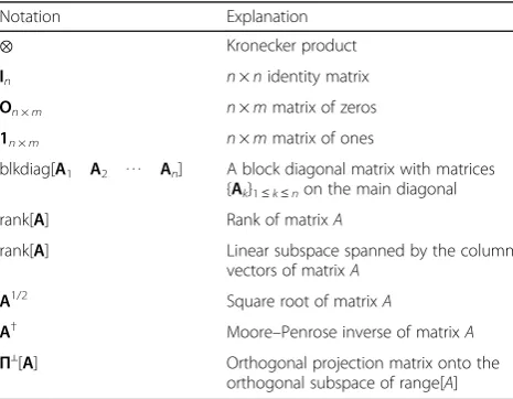
2 Notational conventions and matrix identities In this paper, lowercase and uppercase boldface letters are used to denote vectors and matrices, respectively. The notational conventions that are used throughout this paper are listed in Table1, where the right side de-scribes the definition of some common mathematical notations shown on the left side.
Table2shows four matrix identities, which are useful for the theoretical development in this paper. It contains two orthogonal projection matrix formulas for the full-column-rank matrix, the partitioned matrix inversion formula for symmetric matrix, and the matrix inversion lemma.
3 Measurement model and problem formulation 3.1 Measurement model for target source
We consider three-dimension (3D) localization scenario, in whichMsensors are used to capture the radiated signal from an emitting point source. The sensors are located at positionswm= [xr,myr,mzr,m]
T
(1≤m≤M). The TDOAs of the received signals with respect to the signal at refer-ence sensor, say sensor 1, are estimated to determine the location of the target source. The unknown position of the transmitter is assumed to beu= [x y z]T.
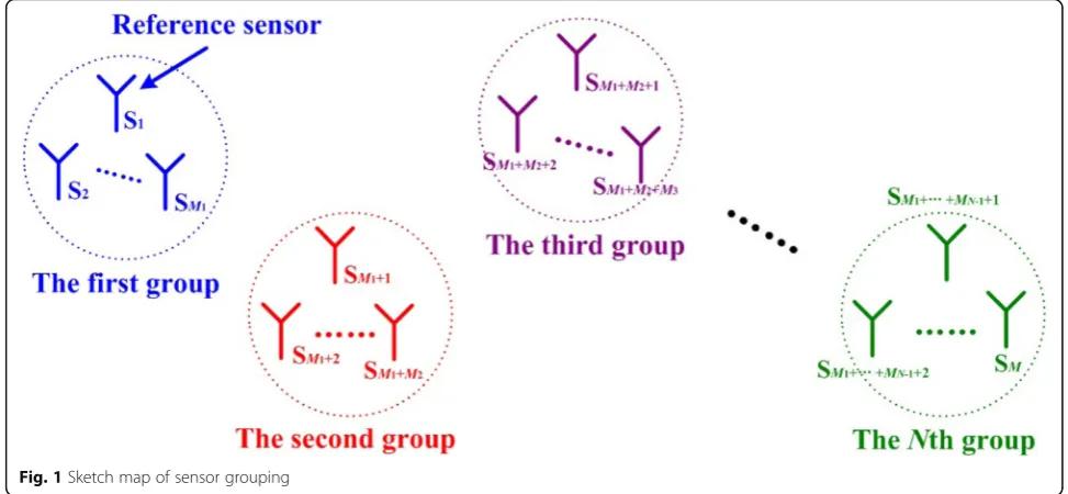
As discussed in [59], perfect synchronization for all sensors may not be feasible if the sensors are widely sep-arated or there are a large number of sensors. However, it is relatively simple to perform synchronous sampling for some of the sensors that are close to each other. For this reason, we can divide the sensors into N groups.
The number of sensors in the nth group is set to Mn, which implies M¼PNn¼1Mn. Within each group, the signals received at the sensors are sampled synchron-ously with respect to a common local clock. But, the clocks from different sensor groups are not the same and clock offsets exist among them. Without loss of gen-erality, the sensors are grouped in the following manner.
In Fig. 1, Sm stands for the mth sensor and S1 repre-sents the reference sensor. Since the reference sensor be-longs to the first group, the clock bias of this group can be assumed to be zero.
It is well known that TDOA measurement can be eas-ily converted to range difference of arrival (RDOA) measurement given the signal propagation speed. There-fore, TDOA and RDOA are used interchangeably throughout this paper. Based on the above assumption, the RDOAs can be modeled as:
^
value in the presence of synchronization errors, εm1 is
the additive noise,ρnis the range offset due to clock bias of group nwith respect to group 1, M~n¼
It is assumed that the error vector ε follows a zero-mean Gaussian distribution with covariance matrix Table 1Notational conventions
Notation Explanation
⊗ Kronecker product
In n×nidentity matrix
On×m n×mmatrix of zeros
1n×m n×mmatrix of ones
blkdiag[A1 A2 ⋯ An] A block diagonal matrix with matrices
{Ak}1≤k≤non the main diagonal
rank[A] Rank of matrixA
rank[A] Linear subspace spanned by the column
vectors of matrixA
A1/2 Square root of matrixA
A† Moore–Penrose inverse of matrixA
Π⊥[A] Orthogonal projection matrix onto the
orthogonal subspace of range[A]
Table 2Matrix identities
Serial
(AandCare symmetric matrices)
II (A+BCD)−1=A−1−A−1B(C−1+DA−1B)−1DA−1
Q= E[εεT]. Note that ρ is the clock bias vector and its unit is meter not second because RDOA is used instead of TDOA. Besides, from the definition of matrixΓ in (3), it can be easily checked that rank[Γ] =N−1.
On the other hand, the accurate sensor locations {wm}1≤m≤M are not known and only noisy versions of them, denoted by f^vmg1≤m≤M, are available. Mathemat-ically, we have
^vm¼wmþξm ð1≤m≤MÞ ð4Þ
where ξm is the position error in ^vm. The collection of
f^vmg1≤m≤M forms a 3M× 1 sensor location vector as
below:
^v¼wþξ ð5Þ
where v¼ ½^vT 1 ^v
T 2 ⋯ ^v
T M
T
and ξ¼ ½ξT
1 ξT2 ⋯ ξTM T
. It is assumed thatξis Gaussian distributed with zero mean and covariance matrix P= E[ξξT]. Moreover, ξ is inde-pendent ofε.
3.2 Measurement model for calibration source
Assume that there exist some calibration emitters that are not far from the target. Moreover, the locations of the cali-bration sources are accurately known. The RDOAs of the calibration signals are also measured based on the sensors given in Fig.1. These measurements are helpful in redu-cing the effects of synchronization offsets and sensor loca-tion errors.
The number of calibration emitters is set to D, and the position of thedth calibration source is denoted as
uc, d= [xc, d yc, d zc, d] T
(1≤d≤D). Since timing synchronization offsets are caused by the difference of
local clocks from different sensor groups, it is reason-able to assume that the clock bias vectorρ remains the same for different signals [79]. As a consequence, the RDOA vector of thedth calibration signal can be writ-ten as:
^rc;d¼rc;dþεc;d¼ f uc;d;w
þΓρþεc;d ð1≤d≤DÞ
ð6Þ
where εc, dis the measurement error, which is modeled as a zero-mean Gaussian random vector with covariance matrixQc,d. Besides,εc;d1 andεc;d2 are statistically
inde-pendent for d1≠d2, and {εc, d}1≤d≤D are uncorrelated withεandξ.
Putting all theDequations in (6) together yields
^rc¼rcþεc¼ f wð Þ þΓρþεc ð7Þ
where
Γ¼1D1Γ ; f wð Þ ¼
f uc;1;w
T
f uc;2;w
T
⋯
f uc;D;w
T
T
^rc¼ ^rTc;1 ^r T c;2 ⋯ ^r
T c;D
h iT
; rc¼ rTc;1 r T c;2 ⋯ r
T c;D
h iT
;
εc¼ εTc;1 εTc;2 ⋯ εTc;D
h iT
8 > > > > > > > > > < > > > > > > > > > :
ð8Þ
It follows from the above assumption thatεcis a zero-mean Gaussian random vector with covariance matrix
3.3 Determination of covariance matrices
Before proceeding further, it must be noted that the the-oretical development requires the knowledge of the co-variance matrices Q, Qc, and P, which may not be known in practice. Fortunately, they can be well esti-mated in real-life application.
First, we discuss how to obtain the covariance matrix of the TDOA measurement. According to [80], it can be found that the TDOA estimated by generalized cross-correlation with Gaussian data is asymptotically normally distributed. Besides, it follows from [81] that the TDOA noise vector in Hahn and Tretter’s estimator is also asymptotically normal. Then, if the noise power spectral densities are similar at sensors, the covariance matrices can be replaced by a matrix of diagonal elements 1 and 0.5 for all other elements according to the analysis in [5]. If this condition is not satisfied, for many estimation methods (such as maximum likeli-hood (ML) estimator), Q and Qc approach the CRB under Gaussian noise, and it has explicit form as shown in [82,83].
Second, the covariance matrix of sensor location errors can be obtained by a large number of off-line observations. Specifically, it can be estimated during calibration by using a source of known location and by measuring the amounts of perturbations in the sensor positions. The detailed esti-mation method can be found in [84, 85]. On the other hand, according to the discussion in [24], some scattering models from the environment may also help to determine the covariance matrix.
Although there is no mathematically substantiated ar-gument to support that the approximation of covari-ance matrices does not introduce much loss in accuracy, some previous work indicates that the per-formance degradation due to the approximation is in-significant [86, 87]. The detailed sensitivity of the inaccurate knowledge ofQ, Qc, and P on the perform-ance of the proposed estimator can be considered as a subject for further study. Once the covariance matrices mentioned above are obtained, or well estimated from the estimation methods, we can use them for source localization.
3.4 Problem formulation
In this work, two important problems need to be stud-ied. First, we intend to determine the performance gain in parameter estimation accuracy due to the introduc-tion of calibraintroduc-tion emitters. This problem can be solved by deriving and analyzing the CRB expressions. Second, it is necessary to present an effective method that can provide the estimates of u, w, andρ as accurate as pos-sible with the help of RDOA measurements from the calibration sources.
4 CRB derivation and analysis
It is well known that the CRB establishes a lower bound on the error covariance matrix for any unbiased estimate of a parameter vector. It is often used to investigate the optimality of parametric estimators. This section is de-voted to the derivation of the CRB on the estimation of the parameters of interest. The obtained results can pro-vide some valuable insights into the performance gain for source localization through the introduction of cali-bration signals. Additionally, they can also be considered as a performance benchmark for the proposed solutions in Section5.
4.1 CRB derivation and analysis based on all the RDOA measurements
In this subsection, the CRB on the covariance matrix of parameter estimation is deduced based on the RDOA mea-surements from both target source and calibration emit-ters. In this situation, the observations consist of^r,^v, and ^rc, and the unknowns includeu,ρ, andw. Hence, we need to define the data vectorη¼ ½^rT ^vT ^rTcTas well as the parameter vectorμ= [uT wT ρT]T. Under the assump-tions stated in Section3, the logarithm probability density function (PDF) ofηparameterized onμis given by
lnðpðηjμÞÞ ¼L−1
2ð^r−f uð ;wÞ−ΓρÞ
TQ−1ð^r−f uð ;wÞ−ΓρÞ
−1 2ð^v−wÞ
TP−1ð^v−wÞ
−1
2 ^rc−f wð Þ−Γρ
T
Q−1
c ^rc−f wð Þ−Γρ
ð9Þ
whereLis a constant independent ofμ. It can be readily verified from (9) that
∂ lnðpðηjμÞÞ
∂μ ¼
F1ðu;wÞ ð ÞTQ−1ε
F2ðu;wÞ
ð ÞTQ−1εþF wð ÞTQ−1
c εcþP−1ξ
ΓTQ−1εþΓTQ−1 c εc
2 6 4
3 7 5
ð10Þ
where F1ðu;wÞ ¼∂f∂ðuuT;wÞ , F2ðu;wÞ ¼ ∂fðu;wÞ
∂wT , and
FðwÞ ¼∂fðwÞ
∂wT . Using (10), we can obtain the CRB matrix for μas
For convenience, we define the matrices
Then, applying the matrix identities I and II in Table2
yields
to the introduction of calibration sources. For this purpose, it is necessary to compare CRB(u) with the CRB of u for the case without calibration emitters. This CRB is denoted as CRBo(u), and it can be
It is straightforward to verify from the third equality in (12) and (15) that
which combined with the first equality in (13), (14) and the matrix identity (II) in Table2leads to
CRBoð Þu−CRB uð Þ ¼X−1Y Zo−YTX−1Y
Before proceeding, some remarks are in order.
4.1.1 Remark 1
The term on the right side of (17) represents the perform-ance improvement resulted from the utilization of the cali-bration sources. It is clear that if Q−c1=2→O, then
CRBo(u)→CRB(u), which means that there is no improve-ment in the localization accuracy. This is not unexpected because Q−c1=2→O implies that the RDOA measurements of the calibration emitters are so noisy and become useless.
4.1.2 Remark 2
fact, the resulting performance gain is considerable at typical measurement error level, as illustrated in the simulation section.
4.1.3 Remark 3
In Appendix 1, we provide an alternative expression for
CRB(u) as follows:
Note that this CRB expression is useful for the per-formance analysis in Section6.2.1.
4.1.4 Remark 4
In Appendix2, the explicit expressions for CRB
the subsequent theoretical development. In addition, it is worthy to point out that all the CRBs obtained above are uncorrelated withρ.
4.2 CRB derivation and analysis based on the RDOA measurements of calibration signals
The aim of this subsection is to derive the CRB on the estimation of parameters ρ and w based on the RDOA measurements from the calibration emitters only. The
associated CRB matrix is denoted by CRBc
ρ w
. In
this situation, the observation and parameter vector should be defined asηc¼ ½^vT ^rTcT andμc= [wT ρT]T, respectively. It follows from the assumptions described in Section 3 that the logarithm PDF of ηc conditioned onμccan be written as:
which means that the RDOA measurements from the target source can be exploited to improve the optimum estimation accuracy forwandρ.
On the other hand, applying the matrix identities (I–III) in Table2yields
CRBcð Þ ¼w F wð Þ
It is noteworthy that these two CRB expressions are useful for the theoretical analysis in Section 5.2. In addition, it can be easily observed from (24) and (25) that bothCRBc(w) andCRBc(ρ) are independent ofρ.
5 Proposed TDOA localization methods
the clock bias can be further refined compared to the esti-mates in the first step.
5.1 Stage 1 of the proposed methods
In the first stage, the measurement vectors ^rc and ^v are combined to estimate ρ and w. In order to obtain the optimum accuracy, the ML criterion is adopted, and the corresponding minimization problem can be formulated as:
min
There is no doubt that the conventional Taylor-series it-erative algorithm, as discussed in [8, 88], can be used to solve (26) and jointly estimate ρ and w. However, in this subsection, we would like to present an alternative Taylor-series iterative algorithm, which is able to reduce the num-ber of parameters involved in the iteration. Note that the objective function in (26) is quadratic inρ; hence, the opti-mal solution toρcan be obtained in closed form as below:
^
where subscript“f” is added to emphasize that this is the solution in the first stage. Inserting (27) back into (26) re-sults in the following concentrated objective function:
min
The unknowns that need to be optimized in (28) in-clude w only, and this minimization problem can be solved by the traditional Taylor-series iterative algo-rithm. The corresponding iterative formula is given by
^
where superscriptkindexes iteration number and w^ðfkÞ de-notes the estimate at the kth iteration. If the sequence
fw^ðkÞ
f g1≤k≤þ∞ converges to w^f, then this vector can be
regarded as the solution of sensor locations in the first phase.
When the iteration process in (29) is terminated, the solution ofρcan be immediately determined by
^
At this point, we make two important remarks about the proposed algorithm in the first stage.
5.1.1 Remark 5
In the procedure stated above, the estimation ofwandρ is decoupled and each is estimated sequentially with lower computational complexity.
5.1.2 Remark 6
Bothw^f andρ^f are asymptotically efficient solutions be-cause their performance can attain the CRB derived in Section 4.2. We prove this result in Section5.2 with an analytical manner.
5.2 MSE analysis in the first stage
The aim of this subsection is to deduce the MSE expres-sions ofw^f and^ρf by employing the first-order perturb-ation analysis. Moreover, the two MSEs are proved to asymptotically reach the corresponding CRBs given in Section 4.2. It is worth emphasizing that the MSE ex-pressions for the estimates in the first phase are import-ant because they are used in the second stage.
5.2.1 MSE expression ofw^f
The theoretical MSE of w^f is derived here. Taking the limit on both sides of (29) produces
Fð Þw^f
and ignoring the second- and higher-order error terms leads to
that the second (approximate) equality in (32) exploits the relation Π⊥½Q−1=2
c ΓQ− 1=2
c Γ¼ODðM−1ÞðN−1Þ. It
fol-lows immediately from (32) that
MSEð Þ ¼w^f E ΔwfðΔwfÞT
Therefore, the estimatew^f is asymptotically efficient.
5.2.2 MSE expression of^ρf
This subsection is devoted to deriving the analytical MSE expression of^ρf. Inserting (7) into (30) and neglecting the second- and higher-order error terms, we obtain
ΓT
Two remarks are drawn at the end of this subsection.
5.2.3 Remark 7
The asymptotic optimality of w^f and ρ^f only holds when the RDOA measurements of target source are not used. Hence, the estimation accuracy of sensor locations and clock bias may be further improved in the subsequent phase.
5.2.4 Remark 8
Applying (35), the cross-covariance matrix between ^ρf andw^f is given by
It can be verified from the matrix identity (II) in Table2
that covð^ρf;w^fÞis equal to the lower-left-hand corner of
5.3 Stage 2 of the proposed methods
In the second phase, we combine the measurement vector ^r with the estimates ofwandρin the first stage, denoted by w^f and ^ρf, to locate the target source. Moreover, the estimates in the first step can be further refined. As in the first stage, the ML criterion is utilized again to obtain the asymptotic optimum performance. It is important to note that two dimension-reduction Taylor-series iterative algo-rithms are proposed in the second step.
5.4 The first algorithm
min
It is obvious that this minimization problem can be efficiently solved through the conventional Taylor-series iterative technique. However, for the purpose of reducing the number of parameters in the iterative procedure, we still exploit the dimension-reduction Taylor-series iterative algorithm. Due to the fact that (42) is a quadratic minimization problem with respect to ρ, its optimal solution can be written in closed form as:
where subscript “s1” is used to highlight that this is the solution in the second phase for the first algo-rithm. Putting (44) back into (42) yields the following concentrated minimization problem:
The set of unknown parameters in (45) consists of u
and w, which cannot be decoupled. As a result, they should be jointly estimated by the traditional Taylor-series iterative technique. The associated update formula for parameter estimation is given by
where superscript kdenotes iteration number; u^ðs1kÞ and
^
wðkÞ
s1 are the estimates ofuandwat thekth iteration,
re-spectively. Let lim
Then,u^s1 and w^s1 can be regarded as the final estimates
for target position and sensor locations, respectively. Be-sides, once the convergence criterion is satisfied and the iteration procedure is terminated, the final estimate for clock bias can be explicitly obtained as:
^
Before we proceed, three important remarks concern-ing the procedure described above are concluded.
5.4.1 Remark 9
In optimization problem (45), matrices Ψ1andΨ2are not accurately known because they depend onw, which is to be estimated. In order to overcome this difficulty, we can use the iteration vectorw^ðs1kÞinstead of the true sensor locations, which means thatΨ1andΨ2should be updated at every it-eration step. Let us assume that the approximations ofΨ1 andΨ2at thekth iteration are denoted by Ψ^
ðkÞ
1 and Ψ^
ðkÞ
2 , respectively. The performance analysis in Section 6.1.1
shows that such an approximation does not affect the asymptotic properties of the estimator. Plentiful simulation results also indicate that the estimation accuracy is rela-tively insensitive to the noise in these two matrices.
ΨT are also required for the theoretical analysis in Section6.
5.4.3 Remark 11
Section 6.1.1 proves that the joint estimate u^s1 ^
ws1
can
asymptotically attain the CRB computed by (81). More-over, Section 6.1.2 shows that the solution ^ρs1 is also asymptotically efficient because its performance can achieve the CRB given by (85) before the thresholding effect occurs.
5.4.4 The second algorithm
The aim of this subsection is to present an alternative dimension-reduction Taylor-series iterative formula in which the iteration variable is composed of uonly. The basic idea behind this algorithm is to automatically miti-gate the effects of sensor location errors produced in the first stage, rather than further improving the sensor po-sitions. As a result, the computational load can be reduced.
For this purpose, we use a first-order Taylor- series ex-pansion, leading to the following approximation:
^r≈ f uð ;w^fÞ þΓρþðε−F2ðu;w^fÞΔwfÞ ð50Þ
where the second- and higher-order terms of estimation error Δwf are ignored. It is immediately obvious that the last term F2ðu;w^fÞΔwf can also be regarded as a measure-ment error asε. The ML estimator is therefore given by
min
Likewise, the optimal solution of ρin (51) can also be written explicitly as below:
^
where subscript“s2”is used to emphasize that this is the solution in the second phase for the second algorithm. By substituting (54) into (51), we obtain the following concentrated minimization problem
Similar to (28) and (45), the Taylor-series iterative for-mula for solving (55) can be expressed as:
^
where superscriptkstands for iteration number andu^ðs2kÞ is the estimate ofuat thekth iteration. The convergence result of sequence f^uðs2kÞg1≤k≤þ∞, denoted by u^s2, can be
viewed as the final estimate of target position for the second algorithm. Moreover, once the iteration process is completed, the final solution of clock bias can be expressed in a closed form as:
^
5.4.5 Remark 12
The estimates of sensor locations obtained in the first stage cannot be further refined in this algorithm.
5.4.6 Remark 13
Similar to the solutionsu^s1andρ^s1obtained by the first al-gorithm, the estimates ^us2 and ^ρs2 are also asymptotically efficient. Section6.2proves that the estimation accuracy of ^
us2and^ρs2can attain the CRBs given by (18) and the third equality in (13), respectively, under mild condition.
5.5 Summary of the proposed methods
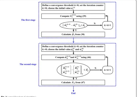
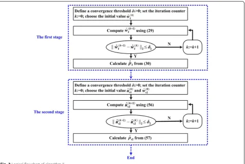
According to the description in Sections5.1 and 5.3, we get two novel TDOA localization algorithms when the TDOA measurements from the calibration emitters are available. Both of them require two stages, and moreover, the first phases of the two algorithms have the same com-putational procedure. In the sequel, we summarize the two newly proposed algorithms, which are called algo-rithm I and algoalgo-rithm II, respectively (Figs.2and3).
We make the following two remarks about the pro-posed algorithms described above.
5.5.1 Remark 14
In the first stage of algorithm I, the initial value w^ðf0Þ can be set to be the available erroneous sensor positions^v. In the second phase of algorithm I, the initial solution w^ðs10Þ can be selected asw^f and the initial guess^uðs10Þ can be ob-tained by the non-iterative algebraic solution proposed in [59]. Simulation results in Section7show that using these initial solutions is able to achieve asymptotically efficient performance. Moreover, this initialization method is also suitable for algorithm II. From our simulation results, it can be observed that fifteen iterations are generally enough to achieve the convergence criterion.
5.5.2 Remark 15
As mentioned in Section 5.4.4, algorithm II involves a smaller amount of computation than algorithm I because the sensor locations are not refined in the second stage of algorithm II. In Appendix 4, we provide the numerical
complexities of the two algorithms, expressed in the num-ber of multiplication operations.
6 Performance analysis of the proposed methods This section is devoted to deriving the theoretical MSE of the TDOA localization methods presented in Section
5. Besides, we prove analytically that the theoretical per-formance of the proposed solutions can reach the corre-sponding CRB accuracy under mild conditions.
6.1 Performance analysis of algorithm I
6.1.1 MSE expression of joint estimatesu^s1andw^s1
The aim of this subsection is to deduce the theoretical
MSE of the joint estimate u^s1 ^ ws1
. We start the derivation
by taking the limit on both sides of (46) as follows:
Q−1=2F1ð^us1;w^s1Þ Q−1=2F2ðu^s1;w^s1Þ
Oð3MþN−1Þ3 Ψ^1
T
Π⊥ Q−1=2Γ
^ Ψ2
Q−1=2ð^r−fðu^s1;w^s1ÞÞ ^
Ψ1 w^f−w^s1
þΨ^2^ρf
¼Oð3Mþ3Þ1
ð58Þ
where Ψ^1¼ lim
k→þ∞Ψ^ ðkÞ
1 and Ψ^2¼ lim
k→þ∞Ψ^ ðkÞ
2 , and we
replaceΨ1andΨ2withΨ^ ðkÞ 1 andΨ^
ðkÞ
2 , respectively, according
to the statement in Remark 9. Putting (2) into (58) and neglecting the second- and higher-order error terms gives
Oð3Mþ3Þ1¼ Q
−1=2F
1ð^us1;w^s1Þ Q−1=2F2ðu^s1;w^s1Þ
Oð3MþN−1Þ3 Ψ^1
T
Π⊥ Q−1=2Γ ^
Ψ2
Q−1=2 f uð ;wÞ−f ^u s1;w^s1
ð Þ þΓρþε
ð Þ
^
Ψ1ðΔwf−Δws1Þ þΨ^2ðρþΔρfÞ
≈ Q−1=2F1ðu;wÞ Q−1=2F2ðu;wÞ
Oð3MþN−1Þ3 Ψ1
T
Π⊥ Q−1=2Γ Ψ2
Q−1=2ðε−F1ðu;wÞΔus1−F2ðu;wÞΔws1Þ
Ψ1ðΔwf−Δws1Þ þΨ2Δρf
ð59Þ
where Δus1¼^us1−u and Δws1¼w^s1−w are the
estima-tion errors in ^us1 and w^s1, respectively. Moreover, it is
worthy to mention that the second (approximate) equality
in (59) makes use of the relation Π⊥
Q−1=2Γ
^ Ψ2
Q−1=2Γ
^ Ψ2
Δus1
which together with (60) produces
MSE ^us1
In Appendix5, we prove that MSE
which immediately implies that the joint estimate ^
us1 ^ ws1
can asymptotically achieve the optimum
performance.
6.1.2 MSE expression of^ρs1
Here, the analytical MSE of ρ^s1 is derived. Inserting (2) into (47) and neglecting the second- and higher-order error terms leads to
ΓTQ−1ΓþΨ^T which means that the solution ρ^s1 is asymptotically efficient.
6.2 Performance analysis of algorithm II 6.2.1 MSE expression ofu^s2
Ωðu^s2;w^fÞ
Inserting (2) into (68) and neglecting the second- and higher-order error terms leads to
O31¼ ðΩðu^s2;w^fÞÞ−1=2 F
Additionally, the second (approximate) equality in
(69) exploits the relation Π⊥
which combined with (52) results in
MSEðu^s2Þ ¼E Δus2ðΔus2ÞT which indicates that the estimate u^s2 has asymptotically optimal accuracy.
6.2.2 MSE expression of^ρs2
Here, we need to derive the analytical MSE of ^ρs2. Sub-stituting (2) into (57) and neglecting the second- and higher-order error terms produces
C1¼ OðN−1Þ3M IN−1
Z−1 O3MðN−1Þ IN−1
C1 IΓ N−1
T
Ωðu;wÞ
ð Þ−1 F1ðu;wÞ OðN−1Þ3
¼ OðN−1Þ3M IN−1
Z−1YT
8 > > < > > :
ð76Þ
Inserting (76) into (75) and usingCRB(u) = (X−YZ−1YT)−1, we have
MSEðρ^s2Þ ¼ OðN−1Þ3M IN−1
Z−1 O3MðN−1Þ IN−1
þ OðN−1Þ3M IN−1
Z−1YTX−YZ−1YT−1
YZ−1
O3MðN−1Þ IN−1
¼CRBð Þρ
ð77Þ
which implies that the solution ^ρs2 is also asymptotically efficient.
Finally, we would like to stress that the performance analysis described above is performed in a general math-ematical framework, which is not limited to a specific signal metric.
7 Numerical experiments
This section presents a set of Monte Carlo simulations to examine the behavior of the proposed TDOA localization algorithms. The root-mean-square error (RMSE) and radius of circular error probability (CEP) are chosen as performance metrics. All the simulation results are averaged over 2000 independent noise reali-zations. It should be pointed out that, to the best our knowledge, there is no existing algorithm that utilizes calibration emitters to improve the localization accuracy for the scenario where both synchronization clock bias and sensor location errors are present. As a result, there are relatively few algorithms that can be directly used for fair performance comparison. Note that, as mentioned in [71], the differential calibration (DC) technique is commonly used in global positioning systems (GPS) to mitigate the effect of uncertainties in satellite position, and various errors caused by satellite clock mismatch and tropospheric and ionospheric layers. Moreover, this method can be easily extended to the localization sce-nario studied here. So, it is reasonable to compare our methods with the DC approach. Additionally, we also compare the performance of the proposed solutions with
the TWLS algorithm in [59], the Taylor-series iterative algorithm extended from [8], and the algorithm in [70], none of which makes use of the calibration emitters. From this comparison, we can clearly observe the performance improvement resulted from the use of the calibration sources. On the other hand, the CRBs de-rived in Section 4 are also used as an important per-formance benchmark, which can corroborate the asymptotic efficiency of the new algorithms.
In the first set of experiments, we compare the radiuses of CEP of the two proposed algorithms with the TWLS al-gorithm in [59], which does not utilize the TDOA measure-ments obtained from the calibration signals. The simulation scenario contains an unknown source located at
u= [4000 4000 4000]T (m) and the localization task is performed by an array ofM= 15 passive sensors. The actual sensor locations are tabulated in Table3, which shows that the sensors are divided into 5 groups. The clock offset vec-tor is set asρ= [20 − 25 15 −10]T(m). Besides, two calibration emitters are deployed near the target source, and they are located at uc, 1= [3200 5800 2500]T (m) and uc, 2= [6200 3800 5600]T (m). In generating the simulation results, the RDOA measurements from the tar-get source and calibration emitters are generated by add-ing to the true values zero-mean Gaussian noise with covariance matrix Q¼σ2
RDOAT and Qc¼σ2RDOATc, re-spectively.T is an (M−1) × (M−1) matrix with diagonal elements equal to 1 and all other elements equal to 0.5;Tc is an D(M−1) ×D(M−1) block diagonal matrix and its diagonal blocks are equal toT. The erroneous sensor posi-tions are created in a similar way using covariance matrix
P¼σ2
PI3M.σRDOAand σPdenote the standard deviations of RDOA measurement errors and sensor position pertur-bations, respectively.
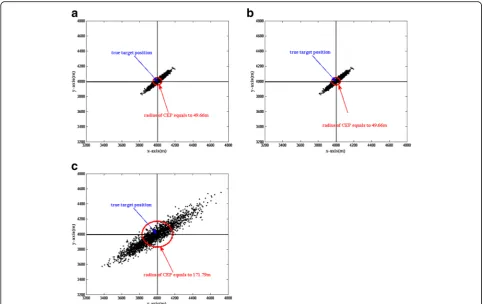
We set σRDOA= 10 (m) and σP= 5 (m). The number of Monte Carlo runs equals 2000. Figs. 4 and 5 show the scatter plots of the source location estimates in thex–yand
y–zplane, respectively. The radiuses of CEP for the three localization algorithms are also provided in the figures.
It can be easily observed from Figs.4and5that the esti-mation performances of the two new algorithms are the same since they have the same radius of CEP. Moreover, the two proposed algorithms can achieve much higher localization accuracy than the TWLS algorithm in [59]. Obviously, the performance improvement in location ac-curacy mainly results from the utilization of the calibra-tion emitters.
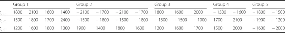
Table 3Sensor positions in the unit of meters
Group 1 Group 2 Group 3 Group 4 Group 5
xr,m 1800 2100 1600 1400 −2100 −1700 −2100 −1700 1800 1600 2000 −1500 −1600 −1800 −1500
yr,m 1500 1800 1700 2400 −1500 −1800 −1500 −1800 −1300 −1500 −1000 1700 2100 −1900 −1200
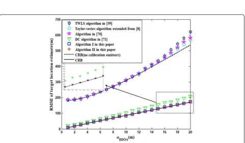
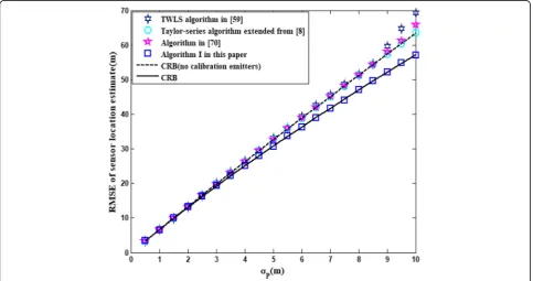
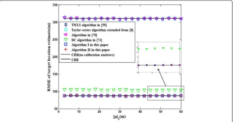
The second set of experiments evaluates the estimation RMSEs of different localization algorithms mentioned above. The simulation parameters are the same as those for the previous experiments, except thatσRDOA,σP, and the norm ofρ(i.e.,‖ρ‖2) are changed. First, the standard deviation of sensor position errors is set toσP= 5 (m) and the clock off-set vector is fixed at ρ= [20 −25 15 −10]T (m). Figs.6,7, and8depict the RMSEs of the estimated target location, sensor position, and clock offset versus σRDOA, respectively. Subsequently, we set σRDOA= 10 (m) and ρ= [20 −25 15 −10]T(m). Figs.9,10, and11show the RMSEs of target location, sensor position, and clock offset estimates as a function of σP, respectively. Next, σRDOAandσP are fixed at 10 (m) and 5 (m), respectively, and the direction of clock offset vector is the same as
ρ= [20 −25 15 −10]T (m). The RMSEs of the esti-mated target location, sensor position, and clock offset against ‖ρ‖2 are plotted in Figs. 12, 13, and 14, respectively.
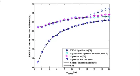
From Figs. 6, 7, 8, 9, 10, 11, 12, 13, and 14, it can be found that the two new algorithms are both asymptotically efficient since they can achieve the relevant CRBs obtained in Section4.1. As a result, the effectiveness of the theoret-ical derivation carried out in Section6can be confirmed. Moreover, the superiority of the proposed algorithms over
Fig. 6RMSE of target location estimate versusσRDOA
norm of clock offset vector, which is consistent with the CRB analysis in Section4.
The third set of experiments studies the effect of the number of calibration sources. Assume that the 3D localization scenario comprises 16 sensors whose true loca-tions are given in Table4. They are used to locate a source
through the RDOA measurements from both target source and calibration emitters. The covariance matrices of the RDOA measurements and sensor location errors are chosen in the same way as previously specified. As shown in Table 4, the sensors are separated into 5 sets and the sensors within the same set are close to each other. The Fig. 7RMSE of sensor location estimate versusσRDOA
clock offset vector is set asρ= [−18 22 −15 24]T(m). The target source is located at u= [5000 5000 5000]T (m), which needs to be estimated with the help of calibra-tion signals. The estimacalibra-tion accuracies of the proposed al-gorithms are examined in three cases. In the first case, a single calibration source is used for target localization,
and the position of this calibration source is given by
uc= [6800 5800 4500]T (m). The second case as-sumes that there are two calibration emitters, which are located at uc, 1= [6800 5800 4500]T (m) and uc, 2= [7200 5500 5600]T (m), respectively. Three calibration sources are deployed for locating the Fig. 9RMSE of target location estimate versusσP
target in the third case and their locations are set asuc, 1= [6800 5800 4500]T(m),uc, 2= [7200 5500 5600]T(m), and uc, 3= [4000 3800 4200]T (m), respectively. Figures15,16, and17illustrate the RMSEs of the estimated target location, sensor position, and clock offset versus
σRDOA, respectively, whenσP= 5 (m). Figures18,19, and20
plot the RMSEs of target location, sensor position, and clock offset estimates as a function of σP, respectively, when σRDOA= 10 (m).
From Figs. 15, 16, 17, 18, 19, and 20, we can observe that the proposed algorithms are shown to yield the so-lutions reaching the CRB accuracy under moderate noise Fig. 11RMSE of clock offset estimate versusσP
level. This finding can further support the theoretical development in Section6. It can also be concluded that, as expected, the parameter estimation accuracy will im-prove when more calibration sources are available for target localization. Moreover, the higher the noise level, the greater the performance gain in localization
accuracy resulted from the increase in the number of calibration signals.
In the fourth experiment, we compare the running time of the proposed algorithms with the other TDOA localization algorithms mentioned above. The simula-tions are carried out using MATLAB R2017b on a Fig. 13RMSE of sensor location estimate versus‖ρ‖2
ThinkPad laptop equipped with Intel Core i7-7500 CPU and 8GB RAM. The simulation settings are the same with those used to produce Figs.4and5. In Table5, the average CPU computational time is compared for the considered localization algorithms.
The results in Table5 show that the TWLS algorithm in [59] takes the least computation time, followed by the Taylor-series iterative algorithm extended from [8] and the algorithm in [70]. This observation is not unexpected because none of these three algorithms take advantage of the measurements from the calibration emitters. More-over, the DC algorithm is more computationally efficient than the two proposed algorithms. The reason is that the DC algorithm does not refine the sensor locations and es-timate the clock bias. Finally, algorithm II is less computa-tionally demanding than algorithm I because the former does not improve the sensor locations in its second stage.
Finally, we would like to point out that although our proposed algorithms require more computation than the other algorithms, the computational complexity is still ac-ceptable when they are executed onboard a node of a wireless sensor network (WSN). There are at least three
reasons. First, the new algorithms have fast convergence rate. Second, the dimension of variables involved in the it-eration is reduced in the proposed algorithms. Third, the algorithms can be implemented through a graphics pro-cessing unit (GPU) chip, which can support parallel opera-tions and has much higher computation speed than CPU chip. It is noteworthy that one of our future works is to implement the new algorithms in a practical WSN.
8 Results and discussions
From the simulation results described above, we can ob-serve that the two proposed algorithms are both asymp-totically efficient because they can achieve the relevant CRBs given in Section4.1. The superiority of the proposed algorithms over the TWLS algorithm in [59], the Taylor-series iterative algorithm extended from [8], and the algorithm in [70] is noticeable. The reason is that the latter three algorithms do not exploit the measurements from the calibration sources. In other words, this signifi-cant performance gap is mainly due to the use of the cali-bration emitters. In addition, it can be seen that the Table 4Sensor positions in the unit of meters
Group 1 Group 2 Group 3 Group 4 Group 5
xr,m 1400 1800 1700 1500 1400 1600 −2300 −1800 −2100 −1900 −1400 −1200 −2000 2100 1600 1900
yr,m 1200 1300 1100 2200 −1300 −2100 1700 1400 1900 −1800 −1600 −1700 −1500 −2000 −1600 −1400
zr,m 2100 1500 1200 1900 1600 2100 1400 1600 2300 −1900 −1500 −2100 −1100 −1700 −2300 −1800
proposed algorithms outperform the DC algorithm and the RMSE improvement increases as σRDOAis increased. This observation is consistent with the analytical result in [71]. More importantly, the DC algorithm cannot further refine the sensor locations and provide the solution for clock bias, while the proposed algorithms can. It can also
be concluded that, as expected, the parameter estimation accuracy improves when more calibration sources are available for target localization. Moreover, the higher the noise level, the greater the performance gain in localization accuracy which resulted from the increase in the number of calibration signals.
Fig. 16RMSE of sensor location estimate versusσRDOAfor a different number of calibration emitters
9 Conclusions
This paper concentrates on the use of a set of calibration signals positioned at known locations when both clock offsets and sensor position errors are present. The localization scenario is similar to the one presented in [59], where the sensors are partially synchronized. The
study begins with the CRB investigation to examine the performance gain due to the utilization of the calibration emitters over the case where the calibration emitters are not available. Some explicit and useful CRB expressions are obtained. The insight gained from the CRB indicates that the calibration sources can significantly reduce the Fig. 18RMSE of target location estimate versusσPfor a different number of calibration emitters
effects of clock bias and sensor position errors. In order to obtain the optimum estimation accuracy, new TDOA localization methods using the measurements from both target source and calibration emitters are developed. Specifically, we propose two dimension-reduction Taylor-series iterative algorithms, both of which have two stages. The first stage estimates the clock offsets and refines the sensor positions based on the calibration TDOA measurements. The statistical characteristic of the noisy sensor locations is also incorporated into this computation procedure. The second stage yields the esti-mates of source location by combining the TDOA mea-surements of target signal and the estimated values in the first phase. The theoretical MSEs of the two pro-posed algorithms are deduced by applying the first-order perturbation analysis. Besides, the proposed methods are proved analytically to reach the CRB accuracy before the thresholding effect takes place. Simulations are con-ducted to support our theoretical development and
demonstrate the superiority of the proposed algorithms over the existing localization algorithms.
Finally, it needs to be mentioned that the present study assumes that the locations of calibration sources are accurately known. In our future work, we intend to extend the proposed algorithms to more practical situa-tions where the exact posisitua-tions of calibration emitters are not available. In addition, we also intend to imple-ment the new algorithms in a practical WSN through parallel GPU acceleration technique.
10 Appendix 1 10.1 Proof of (18)
Combining (11), (12) and the matrix identity (I) in Table2produces
CRB uð Þ ¼ ððF1ðu;wÞÞTðQ−1−Q−1 ðF2ðu;wÞÞ T
ΓT
T
Z−1 ðF2ðu;wÞÞT
ΓT
Q−1ÞF1ðu;wÞÞ −1
ð78Þ
In addition, it can be checked from the third equality in (12) and (19) that
Z¼ ðF2ðu;wÞÞT
ΓT
Q−1 ðF2ðu;wÞÞT
ΓT
T
þΦ−1 ð79Þ
which combined with the matrix identity (II) in Table2gives
Putting (80) back into (78) proves (18). Fig. 20RMSE of clock offset estimate versusσPfor a different number of calibration emitters
Table 5Comparison of the running time
Localization algorithm Average CPU
time (ms)
TWLS algorithm in [59] 3.48
Taylor-series iterative algorithm extended from [8] 14.38
Algorithm in [70] 17.56
DC algorithm 24.32
Algorithm I in this paper 87.87
11 Appendix 2
11.1 Expressions of some CRB matrices
First, using the matrix identity (I) in Table2produces
Subsequently, from (82) and the matrix identity (III) in Table2, we have
Combing (83) and the matrix identity (II) in Table 2
12 Appendix 3
which completes the derivation.
13 Appendix 4
13.1 Numerical complexities of the two proposed algorithms
Tables 6 and 7 list the numerical complexities of the two proposed algorithms, respectively, expressed in the number of multiplication operations.
14 Appendix 5 14.1 Proof ofMSE
Putting (62) and the matrix identity (III) in Table 2
together gives
Besides, from (43), we obtain
Table 6Computational complexity of algorithm I
Stage Computational unit Computational complexity
of each unit
E ΓTQ−1εþΨ2TΦ−1=2 ΔΔwρf
Moreover, it can be checked that
Ωðu;wÞ
Table 7Complexity of algorithm II
Stage Computational unit Computational complexity of each unit Total computational complexity
Stage 1 The same as algorithm I The same as algorithm I
K1 3DðM−1Þð3M
(whereK1andK2 denote the iteration numbers for the dimension-reduction Taylor-series iterative algorithms in the first and second stages, respectively)
range ðΩðu;wÞÞ−1=2 IΓ
which completes the proof.
17 Appendix 8
where the second equality follows from (52). From (101), it can be checked that
Γ
AOA:Angle of arrival; CEP: Circular error probability; CRB: Cramér–Rao bound; CTLS: Constrained total least squares; DC: Differential calibration;
FDOA: Frequency difference of arrival; FIM: Fisher information matrix; FOA: Frequency of arrival; GPS: Global positioning systems; GPU: Graphics processing unit; GROA: Gain ratios of arrival; LOP: Lines of position; MDS: Multidimensional scaling; ML: Maximum likelihood; MSEs: Mean square errors; PDF: Probability density function; QCLS: Quadratic constraint least squares; RDOA: Range difference of arrival; RMSE: Root-mean-square error; RSS: Received signal strength; SI: Spherical interpolation; TDOA: Time difference of arrival; TOA: Time of arrival; TWLS: Two-step weighted least squares; WSN: Wireless sensor network
Acknowledgements
The authors acknowledges the support from the National Natural Science Foundation of China (Grant No. 61201381, No. 61401513, and No.61772548), the China Postdoctoral Science Foundation (Grant No. 2016M592989), the Self-Topic Foundation of Information Engineering University (Grant No. 2016600701), and the Outstanding Youth Foundation of Information Engineering University (Grant No. 2016603201).
Authors’contributions
DW and JY derived and developed the algorithms. XC and CJ conceived of and designed the simulations. XC and JY performed the simulations. DW and FW analyzed the results. DW wrote the manuscript. All authors read and approved the final manuscript.
Availability of data and materials
The datasets generated and/or analyzed during the current study are not publicly available but are available from the corresponding author on reasonable request.
Ethics approval and consent to participate
All data and procedures performed in paper were in accordance with the ethical standards of research community. This paper does not contain any studies with human participants or animals performed by any of the authors.
Consent for publication
Informed consent was obtained from all authors included in the study.
Competing interests
The authors declare that they have no competing interests.
Author details
1National Digital Switching System Engineering and Technology Research
Center, Zhengzhou 450002, People’s Republic of China.2Zhengzhou Institute of Information Science and Technology, Zhengzhou 450002, Henan, People’s Republic of China.3State Key Laboratory of Mathematical Engineering and Advanced Computing, Zhengzhou 450001, Henan, People’s Republic of China.
Received: 5 January 2019 Accepted: 28 June 2019
References
1. K. Doğançay, Bearings-only target localization using total least squares [J]. Signal Processing85(9), 1695–1710 (2005)
2. K. Doğançay, H. Hmam, Optimal angular sensor separation for AOA localization [J]. Signal Processing88(5), 1248–1260 (2008)
3. Y. Wang, K.C. Ho, An asymptotically efficient estimator in closed-form for 3D AOA localization using a sensor network [J]. IEEE Transactions on Wireless Communications14(12), 6524–6535 (2015)
4. J.O. Smith, J.S. Abel, Closed-form least-squares source location estimation from range-difference measurements [J]. IEEE Transactions on Acoustics, Speech and Signal Processing35(11), 1661–1669 (1987)
5. Y.T. Chan, K.C. Ho, A simple and efficient estimator by hyperbolic location [J]. IEEE Transactions on Signal Processing42(4), 1905–1915 (1994) 6. Y. Huang, J. Benesty, G.W. Elko, R.M. Mersereau, Real-time passive source
7. Z. Huang, J. Liu, Total least squares and equilibration algorithm for range difference location [J]. Electronics Letters40(5), 121–122 (2004)
8. L. Kovavisaruch, K.C. Ho,Modified Taylor-series method for source and receiver localization using TDOA measurements with erroneous receiver positions [A]. Proceedings of the IEEE International Symposium on Circuits and Systems [C].
(IEEE Press, Kobe, 2005), pp. 2295–2298
9. K.H. Yang, G. Wang, Z.Q. Luo, Efficient convex relaxation methods for robust target localization by a sensor network using time differences of arrivals [J]. IEEE Transactions on Signal Processing57(7), 2775–2784 (2009)
10. L. Yang, K.C. Ho, An approximately efficient TDOA localization algorithm in closed-form for locating multiple disjoint sources with erroneous sensor positions [J]. IEEE Transactions on Signal Processing57(12), 4598–4615 (2009) 11. K. Yang, J.P. An, X.Y. Bu, G.C. Sun, Constrained total least-squares location
algorithm using time-difference-of-arrival measurements [J]. IEEE Transactions on Vehicular Technology59(3), 1558–1562 (2010) 12. G. Wang, H.Y. Chen, An importance sampling method for TDOA-based
source localization [J]. IEEE Transactions on Wireless Communications 10(5), 1560–1568 (2011)
13. K.C. Ho, Bias reduction for an explicit solution of source localization using TDOA [J]. IEEE Transactions on Signal Processing60(5), 2101–2114 (2012) 14. L.X. Lin, H.C. So, F.K.W. Chan, Y.T. Chan, K.C. Ho, A new constrained
weighted least squares algorithm for TDOA-based localization [J]. Signal Processing93(11), 2872–2878 (2013)
15. Y. Liu, F.C. Guo, L. Yang, W.L. Jiang, An improved algebraic solution for TDOA localization with sensor position errors [J]. IEEE Communications Letters19(12), 2218–2221 (2015)
16. Y.B. Zou, H.P. Liu, W. Xie, Q. Wan, Semidefinite programming methods for alleviating sensor position error in TDOA localization [J]. IEEE Access5, 23111–23120 (2017)
17. K.W. Cheung, H.C. So, Y.T. Chan, Least squares algorithms for time-of-arrival-based mobile location [J]. IEEE Transactions on Signal Processing52(4), 1121–1128 (2004)
18. F.K.W. Chan, H.C. So, J. Zheng, K.W.K. Lui, Best linear unbiased estimator approach for time-of-arrival based localisation [J]. IET Signal Processing 2(2), 156–162 (2008)
19. Ma Z H, Ho K C. TOA localization in the presence of random sensor position errors [A]. Proceedings of the IEEE International Conference on Acoustic, Speech and Signal Processing [C]. Prague, Czech: IEEE Press, May 2011: 2468-2471. 20. M. Sun, L. Yang, K.C. Ho, Efficient joint source and sensor localization in
closed-form [J]. IEEE Signal Processing Letters19(7), 399–402 (2012) 21. J.Z. Li, K.C. Ho, F.C. Guo, W.L. Jiang,Improving the projection method for TOA
source localization in the presence of sensor position errors [A]. Proceedings of the IEEE Sensor Array and Multichannel Signal Processing Workshop [C](IEEE Press, A Coruna, 2014), pp. 45–48
22. N.H. Nguyen, K. Doğançay, Optimal geometry analysis for multistatic TOA localization [J]. IEEE Transactions on Signal Processing64(16), 4180–4193 (2016) 23. K.C. Ho, W. Xu, An accurate algebraic solution for moving source location
using TDOA and FDOA measurements [J]. IEEE Transactions on Signal Processing52(9), 2453–2463 (2004)
24. K.C. Ho, X. Lu, L. Kovavisaruch, Source localization using TDOA and FDOA measurements in the presence of receiver location errors: analysis and solution [J]. IEEE Transactions on Signal Processing55(2), 684–696 (2007) 25. H.W. Wei, R. Peng, Q. Wan, Z.X. Chen, S.F. Ye, Multidimensional scaling analysis
for passive moving target localization with TDOA and FDOA measurements [J]. IEEE Transactions on Signal Processing58(3), 1677–1688 (2010)
26. M. Sun, K.C. Ho, An asymptotically efficient estimator for TDOA and FDOA positioning of multiple disjoint sources in the presence of sensor location uncertainties [J]. IEEE Transactions on Signal Processing59(7), 3434–3440 (2011) 27. F.C. Guo, K.C. Ho,A quadratic constraint solution method for TDOA and FDOA
localization [A]. Proceedings of the IEEE International Conference on Acoustic, Speech and Signal Processing [C](IEEE Press, Prague, 2011), pp. 2588–2591 28. H.G. Yu, G.M. Huang, J. Gao, B. Liu, An efficient constrained weighted least
squares algorithm for moving source location using TDOA and FDOA measurements [J]. IEEE Transactions on Wireless Communications 11(1), 44–47 (2012)
29. G. Wang, Y.M. Li, N. Ansari, A semidefinite relaxation method for source localization using TDOA and FDOA measurements [J]. IEEE Transactions on Vehicular Technology62(2), 853–862 (2013)
30. B.J. Hao, Z. Li, J.B. Si, L. Guan, Joint source localisation and sensor refinement using time differences of arrival and frequency differences of arrival [J]. IET Signal Processing8(6), 588–600 (2014)
31. X.M. Qu, L.H. Xie, W.R. Tan, Iterative constrained weighted least squares source localization using TDOA and FDOA measurements [J]. IEEE Transactions on Signal Processing65(15), 3990–4003 (2017)
32. A. Noroozi, A.H. Oveis, S.M. Hosseini, M.A. Sebt, Improved algebraic solution for source localization from TDOA and FDOA measurements [J]. IEEE Transactions on Wireless Communications7(3), 352–355 (2018) 33. J. Mason, Algebraic two-satellite TOA/FOA position solution on an
ellipsoidal earth [J]. IEEE Transactions on Aerospace and Electronic Systems 40(7), 1087–1092 (2004)
34. K.W. Cheung, H.C. So, W.K. Ma, Y.T. Chan,Received signal strength based mobile positioning via constrained weighted least squares [A]. Proceedings of the IEEE International Conference on Acoustic, Speech and Signal Processing [C](IEEE Press, Hong Kong, 2003), pp. 137–140
35. K.C. Ho, M. Sun, An accurate algebraic closed-form solution for energy-based source localization [J]. IEEE Transactions on Audio, Speech and Language Processing15(8), 2542–2550 (2007)
36. M.R. Gholami, R.M. Vaghefi, E.G. Ström, RSS-based sensor localization in the presence of unknown channel parameters [J]. IEEE Transactions on Signal Processing61(15), 3752–3759 (2013)
37. S. Tomic, M. Beko, R. Dinis, RSS-based localization in wireless sensor networks using convex relaxation: noncooperative and cooperative schemes [J]. IEEE Transactions on Vehicular Technology64(5), 2037–2050 (2015) 38. K.W. Cheung, H.C. So, W.K. Ma, Y.T. Chan, A constrained least squares
approach to mobile positioning: algorithms and optimality [J]. EURASIP Journal on Applied Signal Processing, 1–23 (2006)
39. K.C. Ho, M. Sun, Passive source localization using time differences of arrival and gain ratios of arrival [J]. IEEE Transactions on Signal Processing 56(2), 464–477 (2008)
40. B.J. Hao, Z. Li, J.B. Si, W.Y. Yin, Y.M. Ren,Passive multiple disjoint sources localization using TDOAs and GROAs in the presence of sensor location uncertainties [A]. Proceedings of the IEEE Conference on Communications [C]
(IEEE Press, Ottawa, 2012), pp. 47–52
41. B.J. Hao, Z. Li, Y.M. Ren, W.Y. Yin,On the Cramer-Rao bound of multiple sources localization using RDOAs and GROAs in the presence of sensor location uncertainties [A]. Proceedings of the IEEE Wireless Communications and Networking Conference [C](IEEE Press, Shanghai, 2012), pp. 3117–3122 42. M. Wax, T. Kailath, Decentralized processing in sensor arrays [J]. IEEE
Transactions on Signal Processing33(4), 1123–1129 (1985) 43. D. Dardari, A. Conti, U.J. Ferner, A. Giorgetti, M.Z. Win, Ranging with
ultrawide bandwidth signals in multipath environments [J]. Proceedings of the IEEE97(2), 404–426 (2009)
44. Y. Shen, M.Z. Win, Fundamental limits of wideband localization-part I: a general framework [J]. IEEE Transactions on Information Theory56(10), 4956–4980 (2010)
45. Y. Shen, H. Wymeersch, M.Z. Win, Fundamental limits of wideband localization-part II: cooperative networks [J]. IEEE Transactions on Information Theory56(10), 4981–5000 (2010)
46. A. Coluccia, F. Ricciato, G. Ricci, Positioning based on signals of opportunity [J]. IEEE Communications Letters18(2), 356–359 (2014)
47. F. Bandiera, A. Coluccia, G. Ricci, F. Ricciato, D. Spano,TDOA localization in asynchronous WSNs [A]. Proceedings of the IEEE International Conference on Embedded and Ubiquitous Computing [C](IEEE Press, Milano, 2014), pp. 193–196 48. A. Catovic, Z. Sahinoglu, The Cramer-Rao bounds of hybrid TOA/RSS and
TDOA/RSS location estimation schemes [J]. IEEE Communications Letters 8(10), 626–628 (2004)
49. M. Laaraiedh, L. Yu, S. Avrillon, B. Uguen,Comparison of hybrid localization schemes using RSSI, TOA, and TDOA [A]. Proceedings of the European Wireless Conference [C](IEEE Press, Vienna, 2011), pp. 1–5
50. A. Coluccia, A. Fascista, On the hybrid TOA/RSS range estimation in wireless sensor networks [J]. IEEE Transactions on Wireless Communications17(1), 361–371 (2018)
51. A. Coluccia, F. Ricciato,Maximum Likelihood trajectory estimation of a mobile node from RSS measurements [A]. Proceedings of the IEEE/IFIP Annual Conference on Wireless On-Demand Network Systems and Services [C]
(IEEE Press, Courmayeur, 2012), pp. 151–158
52. A. Tahat, G. Kaddoum, S. Yousefi, S. Valaee, F. Gagnon, A look at the recent wireless positioning techniques with a focus on algorithms for moving receivers [J]. IEEE Access4, 6652–6680 (2016)