F U L L P A P E R
Open Access
Three-dimensional inversion of
magnetotelluric data from the Central
Andean continental margin
Christine Kühn, Jonas Küster and Heinrich Brasse
*Abstract
Magnetotelluric data were collected in the late 1990s in the Central Andes of Chile and Bolivia, with the aim to delineate the electrical conductivity distribution in the subsurface and its relations to subduction processes. In previous studies, these data were interpreted based on 2-D models. The principal result was a vast conductivity zone beneath the Altiplano high plateau at mid and lower crustal depths and a much smaller, though significant conductor associated with the Precordillera Fault System. However, there are some significant 3-D effects in the investigation area, in particular near the coast and on the eastern Altiplano. The aim of this work is to give a reinterpretation based on new 3-D inversion of these data. The 3-D inversion not only provides a better fit to the data compared to 2-D results but furthermore allows to include sites with strong telluric distortion which were ignored in previous studies. We are now able to explain anomalous phases above 90° and induction arrows pointing subparallel to the coast as observed at several sites in the Coastal Cordillera. These strongly distorted data are caused by highly conductive near-surface structures that are partly connected to the Pacific Ocean, forcing currents to flow around the sites. The lower crust beneath the Coastal Cordillera resembles a poorly conductive, nearly homogeneous half-space and is electrically unremarkable. Besides, we can now image the Precordillera conductor as a continuous, elongated feature. The volcanic arc of the Western Cordillera is highly resistive with the exception of a few conductive spots which may be associated with certain individual volcanoes or geothermal resources, respectively. The Altiplano conductor is again the dominant electrical feature in the Central Andes, indicating widespread melting of the middle and lower back-arc crust.
Keywords: Magnetotellurics; 3-D inversion; Subduction zones; Central Andes
Background
In the late 1990s long-period magnetotelluric (MT) data were collected along two profiles at 19.9°S and 21.4°S in Northern Chile and Southwestern Bolivia (see Figure 1). The aim was to infer the electrical conductivity distribu-tion in the subsurface and its reladistribu-tion to subducdistribu-tion pro-cesses at the South American continental margin. Most of the data show typically a 2-D behavior, and consequently, they were interpreted in previous studies based on 2-D models (Brasse et al. 2002; Brasse 2011; Echternacht et al. 1997; Schwalenberg et al. 2002). Nevertheless, some ques-tionable 3-D effects remained which were not taken into
*Correspondence: [email protected]
Freie Universität Berlin, Fachrichtung Geophysik, Malteserstr. 74-100, 12249 Berlin, Germany
account, in particular near the coast and on the Eastern Altiplano. The results introduced here will give a rein-terpretation based on new 3-D inversion by employing the code of (Siripunvaraporn et al. 2005) and ModEM of (Egbert and Kelbert 2012) for the specific investigation areas shown in Figure 1.
The Central Andes developed as a response to the sub-duction of the oceanic Nazca Plate beneath the continen-tal Southern American plate with a velocity approximately 6.5 cm/year and a dip angle of approximately 25° (Klotz et al. 2006). The evolution of the Central Andes is char-acterized by a systematic eastward migration of the mag-matic arc towards the continent (Scheuber et al. 1994).
At the surface, we can distinguish five north-south elongated, main morphological units (Figure 1) starting
Figure 1Map of the investigation area in Northern Chile and Southwestern Bolivia.Red dots indicate the measured magnetotelluric (MT) sites. CC, Coastal Cordillera; LV, Longitudinal Valley; PC, Precordillera; WC, Western Cordillera; EC, Eastern Cordillera. Yellow triangles denote the volcanoes mentioned in the text. Rectangles A (Altiplano), B (Precordillera), and C (forearc) are areas for which 3-D modeling was performed.
with the Coastal Cordillera (CC), the Longitudinal Val-ley (LC), the Precordillera (PC), the Western Cordillera (WC), the Altiplano, and the Eastern Cordillera (EC). The Coastal Cordillera, located currently in a forearc posi-tion, is a relict of the Jurassic-Early Cretaceous magmatic arc. The most prominent structure during this time is the trench-parallel, strike-slip Atacama Fault System that extends for more than 550 km between 21° and 26°S lat-itude (Scheuber et al. 1994). The Longitudinal Valley is a basin filled with Oligocene-Miocene sedimentary and volcanic rocks. The Precordillera developed as a volcanic arc in the Late Cretaceous and Early Paleogene (Scheuber et al. 1994). This area is characterized by a large cover of rhyolitic ignimbrites and domes associated with basaltic and andesitic lavas and intruded by granitoid plutons. A large shear zone, the West Fissure or Falla Oeste, is also located here. Along this zone are encountered some of the largest porphyry copper deposits in the world, e.g., Chuquicamata.
The present-day volcanic arc is located in the West-ern Cordillera. This mountain range reaches mean alti-tudes of about 4,000 m above sea level with volcanic peaks over 6,000 m. It marks the western border of the Altiplano-Puna plateau, characterized by Miocene to recent stratovolcanoes overlying older ignimbrite sheets
of late Miocene eruptions (Baker and Francis 1978; De Silva 1989).
The basement of the Western Cordillera and western Altiplano is formed by Proterozoic metamorphic rocks of the amphibolite facies and igneous rocks of late Paleozoic that are exposed in the Precordillera (Breitkreuz 1986; Wörner et al. 2000). The Altiplano represents an intra-montane basin with Cenozoic continental sediment fill that reach thicknesses of 7 km. In this area of inland drainage, various large salt flats (salars) developed.
The Uyuni-Kenyani Fault System (UKF) consists of three thrust faults (San Cristobal Fault, Corregidores Fault, Uyuni-Kenyani Fault) located in the central part of the Altiplano, with a NNE strike. Here, Paleozoic units are exposed along this major fault zone (Ege 2004). This fault system formed in late Paleogene (28 Ma) and was active again in the Miocene (14 to 10 Ma) and caused an east-vergent thrusting (Elger 2003).
To the east, the Altiplano is bordered by the Eastern Cordillera with its bivergent thrust system in Ordovician sedimentary rocks. The syncline is covered by Tertiary rock units (Ege 2004; Müller et al. 2002).
the Altiplano high plateau in the backarc. Profile segment A extends 190 km from the Western Cordillera across the Altiplano to the large, obliquely running Uyuni-Kenyani Fault System. Investigation area B includes mainly sites from the Precordillera and area C from the Coastal Cordillera and Longitudinal Valley (see Figure 1 (B) and (C)).
Previous studies were based on 2-D models, e.g., (Brasse et al. 2002; Schwalenberg et al. 2002) and (Echternacht et al. 1997). The principal results were a vast zone of par-tial melts beneath the Altiplano at latitude 21°S at mid and lower crustal depths, and the highly conductive West Fis-sure Zone beneath the Precordillera, explained by rising saline fluids from the deeper crust or even the downgoing slab (Echternacht et al. 1997).
Methods
Data and motivation for a 3-D approach
The complex-valued impedance tensorZ links the hor-izontal components of the electric (E in mV/km) and magnetic (Bin nT) fields to each other:
Under ‘normal’ 2-D or even 3-D conditions, the phase ofZxy andZyx should lie in the first or third quadrants, respectively, assuming an exp(iωt) dependence of the inducing fields. This can be derived as a result of Kramers-Kronig relations which connect imaginary and real parts of Z. In the presence of strong 3-D current channeling effects (and also on the seafloor if strong bathymetric gradients occur, even in 2-D), this does not hold any-more, and phases may actually leave the original quadrant (Egbert 1990; Ichihara and Mogi 2009).
In addition to the impedance tensor, the magnetic trans-fer function (tipper)
is particularly prone to 3-D effects. Induction arrows or vectors are derived from the tipper and point away from high-conductivity zones (in the so-called Wiese conven-tion) in a 2-D environment, but generally not above a 3-D subsoil.
A dimensionality analysis (Brasse et al. 2002) described 3-D effects at a number of sites. In particular, some sta-tions on the Eastern Altiplano showed large skew values (as a measure of 2-D vs. 3-D structure) over a large period range. Due to strong distortion with phases above 90°, sites in the Coastal Cordillera were excluded from 2-D interpretation.
Data from the Coastal Cordillera are dominated by the coast effect. A number of sites in this area show high
phases above 90°, indicating telluric distortion effects and current channeling (Lezaeta 2001), which will be analyzed in this paper. An example is shown in Figure 2 for site bla; responses of other sites are displayed in Additional files 1, 2, 3, 4, and 5. Due to the high conductive contrast between the Pacific Ocean and the continent, the induc-tion arrows should point perpendicularly to the coast in W-E direction. However, the arrows strongly deviate from this expected behavior and are basically N-S oriented, indicating a more complex conductivity contrast than a simple 2-D environment (see below).
Earlier 3-D forward modeling of the forearc by (Lezaeta and Haak 2003) showed roughly N-S oriented, conductive structures. It seems that the coast effect is masked by a local anomaly and current channeling. Additionally, a 2-D anisotropic modeling effort by (Beike 2001) yielded a nar-row, anisotropic conductor comparable to the Atacama Fault which may explain the orientation of the induction arrows, but this model could not explain phases above 90°. In previous studies, these sites were thus excluded from 2-D interpretation (Brasse et al. 2002; Schwalenberg et al. 2002).
A similar, unexpected deviation of induction arrows is also observed in the Southern Chilean Andes (Brasse et al. 2009; Kapinos 2011) and in northernmost Chile (Eydam 2008; Galindo 2010). With the help of 3-D inversion, we are now able to explain these effects and the anomalous phases (see below).
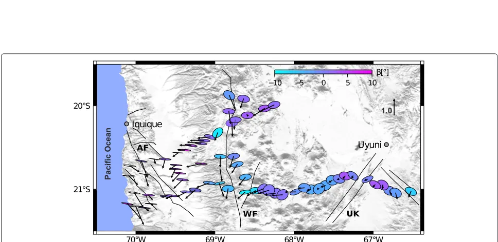
3-D effects are visible on the Altiplano as well. Large impedance skew values and induction vectors pointing obliquely to the profile are characteristic for the east-ern measuring area (Brasse et al. 2002). Figure 3 shows the skew angle β, derived from phase tensor analysis according to (Caldwell et al. 2004). If this value is roughly above +5° or below−5◦, it indicates a 3-D setting of the subsurface. Several sites beneath the Altiplano in area A (see Figure 3) show aβabove 5° over a large range of peri-ods. Furthermore, for longer periods, the orientation of the induction arrows in the Eastern Altiplano seems to be affected by the Uyuni-Kenyani Fault. Note that the aspect ratio of the ellipses deviate significantly between the coast and the inland area, due to the coast effect in the Coastal Cordillera.
It is thus clear that numerous 3-D effects are character-istic for the Central Andean data set. However, it remains unclear to what degree previous 2-D inversions yielded a reliable image of the subsoil. This will be clarified in the following section.
3-D inversion
Figure 2Apparent resistivity and phase curves of an exemplary sitebla.Upper two rows: Apparent resistivity and phase curves of exemplary sitebla, derived from the off-diagonal (left) and the main diagonal (right) elements of the impedance tensorZ. The phases leave the quadrant at 100 s. Below: Induction arrows at sitebla, derived from the real (left) and the imaginary (right) part of the tipper. Blue color represents the data, and red the response after inversion.
• (a) The WSINV3DMT has been developed on a data-space variant of Occam’s inversion introduced for 1-D setting by (Constable et al. 1987) and expanded and implemented for a 3-D case by (Siripunvaraporn et al. 2005). Occam’s approach is an algorithm for generating a smooth minimum norm model to an appropriate fit of the data. The computational costs are reduced by transforming from model-space to data-space and allows to invert data sets on a PC in a manageable time. The version used here is a serial code and does not allow to invert tippers. Smoothness of resistivity variation is
determined by a model covariance with length scales set to 0.1 as default (see also Additional file 6).
• (b) The ModEM inversion algorithm employs the non-linear conjugate gradient method (NLCG). The memory-efficient NLCG and hybrid schemes make the program efficient enough to deal with large data sets (Egbert and Kelbert 2012). Additionally to the impedance tensor, it allows to invert the magnetic transfer function (tipper).
The program includes a variant of the master-worker parallelization over forward problems following the scheme of (Meqbel 2009). This is implemented using calls of the standard Message Passing Interface (MPI), which allows to communicate between different processors and to build a network that is able to use the memories of several processors (Kelbert et al. 2014). In contrast to WSINV3DMT, the covariance matrix allows a manual selection of smoothing for each cell, which, e.g., is use-ful for influences of small-scale near-surface structures (Kelbert et al. 2014).
We have implemented the code on Windows Core-i7 PCs in a local area network (LAN). For the inversion results below, we generally used full impedance data (and tipper with ModEM) in the period range 10 to 10,000 s and discarded those of poor quality, i.e., large scatter. We further reduced the data set by only considering every sec-ond period, resulting in four periods per decade. If not otherwise mentioned, the error floor was set to the default of 5%. Further information on the used smoothing param-eters, number of iterations and resulting root mean square (RMS) are listed in Additional file 6. The construction of the initial models was greatly simplified with the Grid3D software, provided by N. Meqbel (personal communica-tion). In the following sections, we will present selected results of both inversion codes.
Results
Profile A: Altiplano
Investigation area A comprises the easternmost 190 km of the ANCORP profile, extending across the entire plateau from the Western to the Eastern Cordillera. Data from
22 magnetotelluric sites were used. The four complex impedance and the two complex tipper components were first inverted with the ModEM code. The model consists of 55×63×30 cells in thex,y, andzdirections. Each cell spans 4,000 m in the horizontal direction and 100 m in the vertical direction at the surface with an increasing factor of 1.3 to the bottom of the model at 800 km. The initial model was set to a background resistivity of 100m. The final model is shown in Figure 4a,b (see Additional file 7 for a distribution of RMS for each site) in plan view for depths of 1.76 and 37.15 km and as depth sections along profile A in Figure 5.
For comparison, the WIN3DINVMT code was applied to this data subset, too. The same initial model was used for the inversion programs. Figure 5 shows the resistivity distribution with depth of investigation area A, together with an exemplary data fit of sitevad. The left model rep-resents results of the ModEM (root mean square error (RMS) = 1.79) algorithm, the right one of WSINV3DMT (RMS = 1.59) inversion. Both models show mainly similar structures, only the smoothness and depth of the resis-tivity variations are slightly different. It is not surprising that the RMS is slightly larger for the ModEM result as this implies more data with different resolution capabil-ities. RMS is more or less equally distributed over the study area (see Additional file 7); this holds also for the other areas shown later. Although we invert profile data only, artifact off-line structures are practically absent here and for small-depth (short periods) resistivity distribution looks at least plausible (i.e., correlates with morphology and geology).
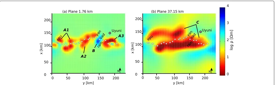
Distinct major and minor basins dominate the resistiv-ity image at shallow depths (see Figure 4a, A1 to A3). The very low resistivities are caused by saline fluids in the salt pans, the largest being the Salar de Uyuni. A highly resistive structure cuts through the conductors between sites ram and yan (see Figure 4a, (B) and Additional file 1). We explain this resistor with the Paleozoic uplift of highly resistive rocks along the Uyuni-Kenyani Fault System. Previous studies were not able to constrain this structure more precisely. Contrary to expectation, the Uyuni-Kenyani Fault Zone is not associated with an iso-lated and elongated conductive zone, neither at small nor large depth.
At depths of more than 20 km, a huge conductivity anomaly (see Figure 4b, (C)) can be seen. This Altiplano Conductivity Anomaly is itemized in other scientific stud-ies and explainable as the northern extension of the source region of the Altiplano-Puna Volcanic Complex (De Silva 1989). The lower boundary is poorly resolved.
N N
Figure 43-D model, obtained with the ModEM scheme (RMS = 1.79) of area A with a background resistivity 100m.(a)Top view at a depth of 1.76 km. A1 to A3, conductive sediments; B, resistive anomaly correlating with morphological elevation, probably Uyuni-Kenyani Fault Zone as well as in(b)in a depth of 37.15 km with Altiplano Conductivity Anomaly (C).
well-conductive structures to the background resistiv-ity, starting the inversion over, and checking the model response. It is thus possible that this conductor extends through the entire crust.
The conductive structure accumulates into two elon-gated structures north and south of the sites. Probably by adding another transect parallel to the ANCORP pro-file, the Altiplano Conductivity Anomaly would be seen as a continuous body. The N-S extension of the Altiplano Conductor can be detected in the northern part of the investigation area (Figure 1 (B)) but is limited there due to missing sites on the central and eastern parts of the Altiplano.
Concluding, the new 3-D inversions generally confirm the previous 2-D results. These are the Altiplano Conduc-tivity Anomaly beneath the plateau and the generally more resistive volcanic arc.
Area B: Precordillera
Area B covers the Pre- and Western Cordilleras between the two profiles. The model consists of 45 × 58× 30 cells in x, y, and z directions. The present volcanic arc at the western margin of the Altiplano correlates with a zone of generally high resistivity (see Figure 6b, (H); for RMS distribution of the study area, see Additional file 9) throughout the entire study area between 19.9°S and 21.4°S as in previous 2-D modeling.
Surprisingly, a good conductor can now be detected in the vicinity of the volcanic arc close to stationsinc,que, jac, and epu (see Additional files 1 and 2 for a plot of responses and data fit). This structure becomes clearly visible at a depth of about 2 km and terminates between 5- and 7-km depths (see Figure 6a, (E)). Here, fumarolic activity is reported at three potentially active centers: the Irruputuncu, Olca, and Paruma volcanoes (Gonzalez-Ferran 1994). This is a new finding compared to earlier
2-D models which could in principal not take the spa-tial distribution of hydrothermal sources into account. Of course, we cannot resolve the exact location nor the true resistivity of these anomalies as they are slightly off-set from the sites. More measurements in Bolivia would be necessary to constrain those potential geothermal resources.
The most prominent conductor in this part of the Cen-tral Andes runs along the Precordillera and is most likely associated with the West Fissure Fault System (Figure 6c, (F) and (G)). It was formerly only modeled as a conductive spot in the upper crust, but we see now that this elon-gated structure reaches much deeper and may even be electrically connected to the slab, although this cannot be resolved uniquely. In the S-N section of the 3-D model (Figure 6c, (F)), it seems that it reaches closer to the sur-face in the north of the study area. These details, as the exact locations of the anomalies in the volcanic chain, are not really resolvable for the time being due to the lack of sites.
The Precordillera conductor was clearly recognized already by (Brasse et al. 2002) and (Schwalenberg et al. 2002) and interpreted as an accumulation of aqueous flu-ids, released from hydrous materials by the subduction process and rising through a conduit provided by the West Fissure Zone. Its location in front of the arc is a com-mon feature of many subduction zones, and there exists a certain correlation with reflection seismological find-ings along the ANCORP line (see the ‘Discussion’ section). The prominent Altiplano conductor illuminates the east-ern margin of the model at depths>30 km but is of course not resolvable with the chosen model block.
Area C: Western Forearc
Figure 5Resistivity distribution with depth along investigation profile A (upper two images).A1 to A3, well-conducting sediments; B, area of high resistivity correlative to the Uyuni-Kenyani Fault; C, Altiplano Conductivity Anomaly. Lower images: Apparent resistivity and phases of the exemplary sitevadof off-diagonal (red and blue) and on-diagonal (pink and green). Left: ModEM, right: WIN3DINVMT.
proximity of the Pacific Ocean with a trench of nearly 8-km depth which leads to a very significant coast effect. We used the ModEM code to invert all horizontal and ver-tical components. In the first step, we inverted only Tzx and Tzywithout impedance data. The best resulting model was then taken as a start to invert all data, i.e., tippers and impedances.
The model core of area C (see Figure 1) extends laterally 250 km in E-W direction, 100 km in N-S direction, and extends to a depth of 634 km vertically. We discretized this area into 63×92×34 cells inx,y, andzdirections. The thickness of the first layer is around 50 m, increasing with a factor of 1.2 inzto the bottom of the model. In the starting model, a background resistivity of 1,000m was set here because of the high resistivity beneath the ocean
and in the Coastal Cordillera at crustal and mantle depths as derived from previous 2-D studies. Furthermore, the Pacific Ocean was added with simplified bathymetry and a resistivity of 0.3m. Fourteen periods spaced between 10 and 104s of 31 stations were used for the inversion, with an error floor of 5% for all elements.
(a) Plane 3.20 km (b) Plane 12.79 km
Figure 63-D model (RMS = 1.79) of area B inverted with WSINV3DMT.Background resistivity set to 100m.(a)Plan view at a depth of 3.20 km. E, conductive structure correlating with fumarolic activity of Olca volcano (triangle).(b)Same model at a depth of 12.79 km. F and G, mark elongated shapes of the West Fissure; H, resistive Western Cordillera.(c)Lower image: S-N transect with depth along the West Fissure. Plate boundary is at approximately 90 km deep (Yoon et al. 2009).
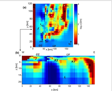
of 3.2 km. At depths below approximately 12 km, the 3-D model is more or less a homogeneous, poorly conductive half-space (see Figure 7b, (L); for the RMS distribution in the measuring area, see Additional file 10).
Sites close to the coast are affected by the Pacific Ocean and display a strong coast effect (strong split of TE and TM modes). However and as mentioned above, some sites are significantly influenced by telluric distortion effects (Lezaeta 2001). Sites with phases leaving the first quad-rant (see Figure 7a, black dots) are mainly located in the Coastal Cordillera (see Figure 7 (CC)). It seems that near-surface structures are at least partly connected electrically with the Pacific Ocean (see Figure 7 (J)). This connection forces the original TE currents to flow around the sites (channeling effects), resulting in those anomalous phases (c.f. Egbert 1990; Ichihara and Mogi 2009). The model not only explains the phases but also the deviated induction arrows at all sites in the Coastal Cordillera.
Sitesglo,pen, andgerare located at the northern seg-ment of the Atacama Fault Zone in the vicinity of the Salar Grande (see Additional files 3 and 5). These three sites show a similar behavior with respect to phases and apparent resistivities like the exemplary station shown in Figure 2. At the surface of this dry, pure halite salar,
numerous strike-slip, reverse, normal faults, extensive cracks, and drainage patterns are found (Allmendinger and Gonzales 2010; Chong et al. 1999) which, if only moderately conductive compared to the salar itself, pro-vide a natural explanation of distortion, together with the observed conductive connection to the Pacific Ocean (see Figure 7 (J)). Additionally, conductive near-surface sed-iments that are younger than the Cordillera basement rocks force current channeling effects.
Site qch located in the Chacarilla gorge at the east-ern margin of the Longitudinal Valley shows also phases leaving the quadrant (see Additional file 4). The trend of this canyon seems to connect the conductive surface sediments of the Longitudinal Valley with the highly con-ductive West Fissure Zone (see Figure 7a,b (K)). The sur-rounding igneous rocks display high resistivity. This large conductivity contrast forces currents to flow along the gorge, resulting in anomalous phases. The same behavior is observed at site685(see Additional file 4) located in a canyon between Longitudinal Valley and Precordillera.
0
log ρ [Ωm]
0 1 2 3 4
50 100 150
20
40
60
80
100
120
0
PO
K
J
N
pen roj
bla
qch 685
glo ger
CC
LV
x [km]
y [km]
0
5
10
15
20
0 20 40 60 80 100 120 140
L
K
K1
K2
J
W E
CC
LV
(a)
(b)
x [km]
z [km]
Figure 73-D model (RMS = 1.91) of the forearc (area C).Background resistivity was set to 1,000m. PO, Pacific Ocean with a resistivity of 0.3
m; CC, Coastal Cordillera; LV, Longitudinal Valley; J, connection with the Pacific Ocean and highly conductive anomalies in the Longitudinal Valley and near Chacarilla canyon; K, near Chacarilla canyon.(a)A plan view at a depth of 3.2 km of the resistivity distribution. Near-surface structures partly connect to the Pacific Ocean and force currents to flow around sites, resulting in phases leaving the quadrant (c.f. (Ichihara and Mogi 2009)). Black dots: sites with phases>90◦.(b)Resistivity distribution with depth along investigation area C at latitude 21◦S. Beneath 12-km depth, the 3-D model resembles a rather homogeneous, poorly conducting half-space (L). K, K1, K2 - West Fissure zone.
point to the west, away from the conductive West Fissure zone.
Discussion
In general, the two applied inversion algorithms, when tested, yielded quite similar results. We could usually achieve a good fit of all components of the impedance tensor and, with ModEM, also of the tipper. This is quite remarkable taking the often much larger scatter of main diagonal data into account. Fit of tipper data very close to the coast is not perfect, but this may be attributed to insufficient consideration of true bathymetry and shape of the coastline. Near-surface resistivity distribution often looks chaotic, but we could almost always associate
scattered conductors with known structures, e.g., small sub-basins. Although the site density is by no means perfect in many parts of the Central Andes, we believe that the foregoing results are a significant improvement over the older 2-D models. Confidence in the results was also achieved by conducting a number of sensitivity tests; owing to limited computing resources, they were of course less extensive than one usually carries out in 2-D environments. The main findings and the most significant differences compared to previous work are as follows:
Forearc: Coastal Cordillera:
The observed phases above 90◦ and induction arrows
meandering features in the Coastal and Precordillera (shown in Figure 8) , the connection to the Pacific Ocean, high conductivity contrasts between younger near-surface structures (Atacama Fault Zone), and highly resistive material from the late Mesozoic magmatic arc (shown in Figure 7).
Thus, our 3-D model explains the strongly anomalous data in the Coastal Cordillera with purely local effects. Note, however, that the deflection of induction arrows is a regional phenomenon and observable over at least 1,000 km from Arica in the north to Tocopilla in the south of our study area (Brändlein 2013; Brasse and Eydam 2008). With current computing capacities, it is not possible to include all available North Chilean forearc data into a single 3-D model, and we are unable to decide for the time being if a local or a regional approach is more appropriate for the North Chilean margin. A regional-scale effect is implicitly contained in a 2-D anisotropic model as presented, e.g., by (Galindo 2010) for tipper data near Arica and perhaps the truth lies in a synthesis of an anisotropic and a 3-D model. The deeper forearc beneath the Coastal Cordillera is highly resistive and resembles an almost unstructured half-space. This is similar to older 2-D models and consis-tent with abundant seismicity in the whole (brittle) crust as discovered very recently (Bloch et al. 2014).
Unlike our model, for data farther south, (Brändlein 2013) shows a conductor in the mantle wedge above the Nazca plate which he attributes to fluid relocation after the 2007 Mw = 7.7 Tocopilla earthquake. Our study area is located directly where the 2014 Mw = 8.2 Iquique earthquake occurred, and we think it is an interesting speculation that now, in the aftermath of this event, such a conductor might appear, too.
Forearc – Precordillera:
The West Fissure Fault System is now imaged as a con-tinuous lineament and with a larger depth extent than previously deduced. In our new 3-D model, this conduc-tor is seen a little closer to the surface, i.e., commencing at 12-km depth instead of 15 km and even less in the north.
Such a conductive structure some tens of kilometers trenchward of the volcanic front is a common feature of many subduction zones and is interpreted as an accu-mulation of fluids originating in the downgoing slab (Worzewski et al. 2011). A reflection seismological study (Yoon et al. 2009) infers a fluid flow from the Nazca slab at this location but with a significantly deeper upper boundary of reflections (approximately 40 km). From there, (Yoon et al. 2009) postulate a bifurcation of fluid flow, subvertically towards the surface and laterally along the so-called ‘Quebrada Blanca Reflector’ (a significant seismic bright spot) towards the volcanic arc. As our model experiment are compatible with such a deep reach-ing conductive structure (even with havreach-ing in mind the
reduced resolution capabilities of MT with respect to lower boundaries of conductive zones), we can for the first time reconcile the seismic and magnetotelluric observa-tions. It remains enigmatic, however, why seismology sees the top of the fluid accumulation zone significantly lower than our MT model. Furthermore, we do not resolve a fluid channel directed towards the arc volcanoes. Thus, a corresponding explanation of the Quebrada Blanca reflector is not consistent with MT observations.
Volcanic arc:
Contrary to earlier expectation, the volcanic arc in the Central Andes is not underlain by large high conductiv-ity zones, neither in the upper nor in the lower crust. This means that a large-volume magma chamber does not exist, at least where our profiles cross the volcanic chain. This even holds for potentially very active volcanoes like Lascar (Díaz et al. 2012). The only exception has been the Lazufre complex where rising partial melts lead to an uplift of 3 cm/year over a large area (Budach et al. 2013).
This was delineated earlier (Brasse 2011) and is now cor-roborated by our new 3-D modeling efforts. Only north of Olca and east/northeast of Irruputuncu volcanoes near-surface high conductivity spots are detected, which are likely manifestations of hydrothermal resources.
Altiplano:
The 3-D model confirms the resistivity image deduced earlier, particularly the Altiplano conductor in the mid to lower crust. It is of enormous dimensions and has recently been detected further south as well (Comeau et al. 2013). All geophysical data hint at widespread melting, including a low-velocity zone as inferred from seismic tomography (Heit et al. 2008). The upper boundary of the Altiplano Anomaly correlates with the Andean Low-Velocity Zone proposed by (Yuan et al. 2000). By inverting gravity data, (Del Potro et al. 2013) assume for an area at latitude 21.5°S to 23°S partially molten rocks that ascend diapiri-cally through a strongly weakened crust up to the surface. For further discussion on this unique anomaly, we refer to (Schilling et al. 2006).
The weak 3-D effect in the Eastern Altiplano may be explained with a resistive structure that is associ-ated with an uplift of resistive older, Paleozoic rocks along the oblique Uyuni-Kenyani Fault Zone. A con-ductive fault zone as in the Precordillera is not found here. Thus, the Uyuni-Kenyani Fault Zone cannot be regarded as a fluid conduit nor as a deposit for magmatic hydrothermal ores.
Conclusions
2520 s
(a)
(b)
Figure 8Map of the investigation area C.Shown are real induction arrows (blue, data; red, response)(a)for a period of 744 s and(b)for a period of 2,520 s. AF, Atacama Fault; WF, West Fissure.
observations near the North Chilean coast (frequent phases above 90° and induction arrows pointing obliquely or even parallel to the coast) are now explained by highly conducting, meandering current pathways rather close to the surface. The West Fissure mega shear zone is imaged as an elongated, deep-reaching conductor promoting fluid
Our new 3-D inversion efforts are a step forward toward explaining the electrical resistivity structure of the mar-gin. More data are needed to resolve certain features particularly in the forearc; this forms a future task.
Additional files
Additional file 1: Data example of investigation area A.Apparent resistivity and phase curves of exemplary sitesepu,yan, andramwith a RMS = 1.59. Derived from the off-diagonal (left) and the main diagonal (right) elements of the impedance tensorZ. Inverted with WSINV3DMT. Additional file 2: Data example of investigation area B.Apparent resistivity and phase curves of sitesjac,que, andincwith a RMS = 1.79. Derived from the off-diagonal (left) and the main diagonal (right) elements of the impedance tensorZ. Inverted with WSINV3DMT.
Additional file 3: Data example incl. induction arrows of investigation area C.Apparent resistivity and phase curves of sitesgloandgerwith a RMS = 1.91. Derived from the off-diagonal (left) and the main diagonal (right) elements of the impedance tensorZand tipper. Inverted with ModEM. Additional file 4: Data example incl. induction arrows of investigation area C.Apparent resistivity and phase curves of sites685 andqchwith a RMS = 1.91. Derived from the off-diagonal (left) and the main diagonal (right) elements of the impedance tensorZand tipper. Inverted with ModEM.
Additional file 5: Data example incl. induction arrows of investigation area C.Apparent resistivity and phase curves of sitespenandrojwith a RMS = 1.91. Derived from the off-diagonal (left) and the main diagonal (right) elements of the impedance tensorZand tipper. Inverted with ModEM. Additional file 6: General information about the shown models. Overview of parameters for the models mentioned in the text. Displayed are RMS, number of iteration, and smoothing parameter.
Additional file 7: RMS distribution of investigation area A.RMS distribution (color coded) of the Altiplano model shown in Figure 5. Upper plot: for impedances and tipper. Center: for impedances only. Bottom: for tipper only.
Additional file 8: Sensitivity study for investigation area A (Altiplano). Sensitivity study for the depth extend of Altiplano Conductivity Anomaly. (a) W to E transect of investigation area A. Dashed lines (A (82 km), B (62 km), and C (48 km)) mark the boundaries, where the resistivity was set back to the initial background resistivity. (b) The influence to the data fit for an exemplary sitechu. At C (48 km), data fit gets worse for longer periods. Additional file 9: RMS distribution of investigation area B.Upper plot: for impedances and tipper. Center: for impedances only. Bottom: for tipper only.
Additional file 10: RMS distribution of investigation area C.RMS distribution of model shown in Figure 7 (Western Forearc). Upper plot: for impedances and tipper. Center: for impedances only. Bottom: for tipper only.
Competing interests
The authors declare that they have no competing interests. Authors’ contributions
CK carried out the 3-D inversion of the forearc data. JK inverted the backarc data. HB, as the project leader, collected the data and supervised the modeling efforts. All authors wrote, read and approved the final manuscript. Acknowledgements
We are indebted to W. Siripunvaraporn, A. Kelbert, G. Egbert, and N. Meqbel for providing their inversion algorithms. David Martens wrote some of the Matlab plotting routines to visualize inversion output. We thank two reviewers for their comments and recommendations.
Received: 12 June 2014 Accepted: 14 August 2014 Published: 10 September 2014
References
Allmendinger RW, Gonzalez G (2010) Neogene to Quaternary tectonics of the Coastal Cordillera, Northern Chile. Tectonophysics 495:93–110
Baker MCW, Francis PW (1978) Upper Cenozoic volcanism in the Central Andes - Ages and Volumes. Earth Planet Sci Lett 41(2):175–187
Beike J (2001) Studien zur anisotropen Leitfähigkeitsverteilung und ein Versuch zur Erklärung magnetotellurischer Übertragungsfunktionen in der Küstenkordillere Nordchiles, diploma thesis, Inst. für Geol. Wiss., Freie Universität Berlin
Bloch W, Kummerow J, Salazar P, Wigger P, Shapiro SA (2014) High-resolution image of the North Chilean subduction zone: seismicity, reflectivity and fluids. Geophys J Int 197(3):1744–1749. doi:10.1093/gji/ggu084 Brändlein D (2013) Geo-electromagnetic monitoring of the Andean
Subduction Zone in Northern Chile. Dissertation, Freie Universität Berlin Brasse H, Lezaeta P, Rath V, Schwalenberg K, Soyer W, Haak V (2002) The
Bolivian Altiplano conductivity anomaly. J Geophys Res 107(B5):EPM 4-1–EPM:4–14. doi:10.1029/2001JB000391
Brasse H, Eydam D (2008) Electrical conductivity beneath the Bolivian Orocline and its relation to subduction processes at the South American
continental margin. J Geophys Res 113:B07109. doi:10.1029/2007JB005142 Brasse H, Kapinos G, Li Y, Mütschard L, Soyer W, Eydam D (2009) Structural
electrical anisotropy in the crust at the South-Central Chilean continental margin as inferred from geomagnetic transfer functions. Phys Earth Planet Inter 173(1–2):7–16. doi:10.1016/j.pepi.2008.10.017
Brasse H (2011) Electromagnetic images of the South and Central American subduction zones. In: Petrovsky E, Herrero-Bervera E, Harinarayana T, Ivers D (eds) The Earth’s magnetic interior, IAGA Special Sopron Book Series. Springer, Berlin, pp 43–81
Breitkreuz C (1986) Das Paläozoikum in den Kordilleren Nordchiles (21°-25°S). Geotektonische Forschungen 70:1–88
Budach I, Brasse H, Díaz D (2013) Crustal-scale electrical conductivity anomaly beneath inflating Lazufre volcanic complex. Central Andes J S Am Earth Sci 42:144–149. doi:10.1016j.jsames2012.11.002
Caldwell TG, Bibby HM, Brown C (2004) The magnetotelluric phase tensor. Geophys J Int 158:457–469
Chong Díaz G, Mendoza M, García-Veigas J, Pueyo JJ, Turner P (1999) Evolution and geothermal signatures in a Neogene forearc evaporitic basin: the Salar Grande (Central Andes of Chile). Palaeograph Palaeoclimatol Palaeoecol 151:39–54
Comeau MJ, Unsworth MJ, Ticona F (2013) Magnetotelluric images of magma distribution beneath Volcan Uturuncu, Bolivia In: IAVCEI Scientific Assembly. Kagoshima, Japan. 20–24 July 2013
Constable CS, Parker RL, Constable GC (1987) Occam’s inversion: a practical algorithm for generating smooth models from electromagnetic sounding data. Geophysics 52:289–300
De Silva SL (1989) Altiplano-Puna volcanic complex of the central Andes. Geology 17:1102–1106
Del Potro R, Diez M, Blundy JD, Gottsmann JH, Camacho AG (2013) Diapiric ascent of silicic magma beneath the Bolivian Altiplano. Geophys Res Lett 40(10):2044–2048
Díaz D, Brasse H, Ticona F (2012) Conductivity distribution beneath Lascar volcano (Northern Chile) and the Puna, inferred from magnetotelluric data. J Volc Geotherm Res 217–218:21–29. doi:10.1016/j.jvolgeores.2011.12.007 Echternacht F, Tauber S, Eisel M, Brasse H, Schwarz G, Haak V (1997)
Electromagnetic study of the active continental margin in Northern Chile. Phys Earth Planet Inter 102:69–87
Egbert GD, Kelbert A (2012) Computational recipes for electromagnetic inverse problems. Geophys J Int 189:251–267
Egbert GD (1990) Comments on ’Concerning dispersion relations for the magnetotelluric impedance tensor’ by. E. Yee and K. V. Paulson. Geophys J 102:1–8
Ege H (2004) Exhumations- und Hebungsgeschichte der zentralen Anden in Südbolivien (21°S) durch Spaltspur-Thermochronologie an Apartit. Dissertation, Freie Universität Berlin
Elger K (2003) Analysis of deformation and tectonic history of the Southern Altiplano Plateau (Bolivia) and their importance for plateau formation. Dissertation, Freie Universität Berlin
Eydam D (2008) Magnetotellurisches Abbild von Fluid- und Schmelzprozessen in Kruste und Mantel der zentralen Anden. Diploma, Freie Universität Berlin Galindo JC (2010) Anisotropic modelling of magnetotelluric data in North
Gonzalez-Ferran O (1994) Volcanes de Chile, Inst. Geográfico Militar. Santiago de Chile:640
Heit B, Koulakov I, Asch G, Yuan X, Kind R, Alcocer-Rodriguez I, Tawackoli S, Wilke H (2008) More constraints to determine the seismic structure beneath the Central Andes at 21°S using teleseismic tomography analysis. J S Am Earth Sci 25:22–36. doi:10.1016/j.jsames.2007.08.009
Ichihara H, Mogi T (2009) A realistic 3-D resistivity model explaining anomalous large magnetotelluric phases: the L-shaped conductor model. Geophys J Int 179:14–17
Kapinos G (2011) Amphibious magnetotellurics at the South-Central Chilean continental margin. Dissertation, Freie Universität Berlin
Kelbert A, Meqbel N, Egbert GD, Tandonc K (2014) ModEM: a modular system for inversion of electromagnetic geophysical data. Comput Geosci 66: 40–53. doi10.1016/j.cageo 01:010
Klotz J, Abolghasem A, Khazaradze G, Heinze B, Vietor T, Hackney R, Bataille K, Maturana R, Viramonte J, Perdomo R (2006) Long-term signals in the present-day deformation field of the Central and Southern Andes and constraints on the viscosity of the Earths upper mantle. In: Oncken O, Chong G, Franz G, Giese P, Götze HJ, Ramos VA, Strecker MR, Wigger P (eds) The Andes: active subduction orogeny: frontiers in Earth sciences. Springer, Berlin, pp 65–89
Lezaeta P (2001) Distortion analysis and 3-D modeling of magnetotelluric data in the Southern Central Andes. Dissertation, Freie Universität Berlin:177 Lezaeta P, Haak V (2003) Beyond magnetotelluric decomposition: induction,
current channeling, and magnetotelluric phases over 90◦. J Geophys Res 108(B6):2305. doi:10.1029/2001JB000990
Meqbel NM (2009) The electrical conductivity structure of the Dead Sea Basin derived from 2D and 3D inversion of magnetotelluric data. Dissertation, Freie Universität Berlin, p 201
Müller JP, Kley J, Jacobshagen V (2002) Structure and Cenozoic kinematics of the Eastern Cordillera, Southern Bolivia (21°S). Tectonics 21(5):1.1–1.24 Scheuber E, Bogdanic T, Jensen A, Reutter K-J (1994) Tectonic development of
the North Chilean Andes in relation of plate convergence and magmatism since the Jurassic. In: Reutter KJ, Scheuber E, Wigger P (eds) Tectonics of the Southern Central Andes. Springer, Berlin, pp 121–139
Schilling FR, Trumbull RB, Brasse H, Haberland C, Asch G, Bruhn D, Mai K, Haak V, Giese P, Muoz M, Ramelow J, Rietbrock A, Ricaldi E, Vietor T (2006) Partial melting in the Central Andean crust: a review of geophysical,
petrophysical, and petrologic evidence. In: Oncken O, Chong G, Franz G, Giese P, HJ GÃ ˝utze, Ramos VA, Strecker MR, Wigger P (eds) The Andes: active subduction orogeny: frontiers in Earth Sciences. Springer, Berlin-Heidelberg, pp 459–474
Schwalenberg K, Rath V, Haak V (2002) Sensitivity studies applied to a 2-D resistivity model from the central Andes. Geophys J Int 150:673–686 Siripunvaraporn W, Egbert G, Lenbury Y (2005) Three-dimensional
magnetotelluric inversion: data-space method. Phys Earth Planet Inter 150:3–14
Wörner G, Lezaun J, Beck A, Heber V, Lucassen F, Zinngrebe E, Rössling R, Wilke HG (2000) Precambrian and early Paleozoic evolution of the Andean basement at Belén (Northern Chile) and Cerro Uyarani (western Bolivia Altiplano). J S Am Earth Sci 13(8):717–737
Worzewski T, Jegen MM, Kopp H, Brasse H, Taylor W (2011) Magnetotelluric image of the fluid cycle in the Costa Rican subduction zone. Nature Geosci 4:108–111. doi:10.1038/NGEO1041
Yoon M, Buske S, Shapiro SA, Wigger P (2009) Reflection image spectroscopy across the Andean subduction zone. Tectonophysics 472:51–61. doi:10.1016/j.tecto.2008.03.014
Yuan X, Sobolev SV, Kind R, Oncken O, Bock G, Asch G, Schurr B, Gräber F, Rudloff A, Hanka W, Wylegalla K, Tibi R, Haberland C, Rietbrock A, Giese P, Wigger P, Roewer P, Zandt G, Beck S, Wallace T, Pardo M, Comte D (2000) Subduction and collision processes in the Central Andes constrained by converted seismic phases. Nature 408:958–961
doi:10.1186/1880-5981-66-112
Cite this article as:Kühnet al.:Three-dimensional inversion of
magnetotelluric data from the Central Andean continental margin.Earth,
Planets and Space201466:112.
Submit your manuscript to a
journal and benefi t from:
7Convenient online submission
7Rigorous peer review
7Immediate publication on acceptance
7Open access: articles freely available online
7High visibility within the fi eld
7Retaining the copyright to your article