R E S E A R C H
Open Access
Multipath exploited Bayesian and Cram ´er-Rao
bounds for single-sensor target localization
Pawan Setlur
*and Natasha Devroye
Abstract
In urban scenarios, radar returns consist of a direct path return along with multipath returns from signal reflections off surfaces such as building walls or floors. When multipath is resolvable, and given the knowledge of the geometry of the reflecting surfaces, it has recently been demonstrated that multipath returns create additional “virtual” radar sensors, thereby permitting target localization with a single radar sensor. The goal of this article is to determine theoretical variance lower bounds on how well a single-sensor system is able to localize a target in the presence of exploitable multipath and discuss several practical issues that arise in this context, including the multipath association problem, clutter, and the impact of wall roughness. Exploiting multipath, rather than viewing it strictly as a hindrance, is an emerging topic in the radar community whose potential is not yet fully understood. Towards this goal, we first derive the Cram´er-Rao and the Bayesian Cram´er-Rao bounds on target localization using a single-sensor which exploits resolvable multipath. For a wide class of radar-target geometries, functions termed multipath preservers are derived which indicate when multipath is physically observable in the radar returns; these functions assist in evaluating the potential of multipath exploitation in urban sensing. Given a reflecting geometry, the obtained lower bounds allow the radar operator to anticipate blind spots, place confidence levels on the localization results, and permit sensor positioning to optimally aid in exploiting multipath for target localization. It is shown that variance bounds on the location parameters improve with richer resolvable multipath generating mechanisms.
Keywords: Target localization, Radar, Multipath exploitation, Bayesian Cram´er-Rao, Urban sensing, Experimental design, Statistical identifiability
1 Introduction
When radar signals are reflected from building walls in urban scenarios, multipath radar returns result, causing false positives. The objective of multipath exploitation is to identify these multipath returns, which exist because of the target and its surrounding reflecting geometry, and exploit them to improve the radar system perfor-mance. Recently, it has been noted that when multipath returns are resolvable and the reflecting surface geometry is known a priori (e.g., via prior surveillance), multi-path radar returns create virtual radar sensors, permitting non-coherent target localization with asingle-sensor[1]. This single-sensor localization approach may offer a viable sensing solution to modern urban sensing challenges. In other non-radar applications, such as wireless sensor
*Correspondence: [email protected]
Department of Electrical and Computer Engineering, University of Illinois at Chicago, Chicago, IL 60607, USA
localization, the multipath also results in virtual beacons (receivers) similarly permitting localization with a single sensor.
1.1 Goal
Our goal is to better understand the fundamental limits of idealized multipath exploitation in the context of sin-gle sensor systems and to analytically discuss the system performance with practical considerations including for example, the roughness of walls and the presence of clut-ter. Single-sensor systems are covert, may be smaller, sim-pler to deploy, and more cost-effective than multi-sensor systems; however, this simplicity may come at the cost of increased signal processing complexity and/or decreased performance when compared to multi-sensor systems. As little work has emerged on single-sensor multipath exploitation, we focus on the theoretical gains possible here, which could be used as a benchmark for future multipath exploiting localization schemes.
For analytical tractability, the direct path time delay and the multipath time delays are assumed to be normally distributed perturbed versions of their true counterparts. The main crux of this article is in evaluating the poten-tial of single-sensor-based localization from a theoretical perspective using the Cram´er-Rao bounds (CRBs) and the Bayesian Cram´er-Rao bounds (BCRBs). Further, the objective is also to determine spatial regions within a geometry where such systems are most beneficial in local-izing targets via multipath exploitation. The former pro-vides a lower bound on the variance of the non-coherent localization error, whereas the latter determines optimal target or sensor positions where single-sensor radar sys-tems offer the most benefit. Neither of these have yet been addressed for a single-sensor system, and considering practical constraints in the literature.
Towards our goal, we study one particular geometry as an example: a single target enclosed in a rectangular urban canyon. The multipath generating mechanisms, i.e., the walls, are assumed to be smooth at the radar oper-ating frequencies, resulting in specular reflections. The wall roughness and its impact on localization is handled subsequently.
1.2 Contributions
Our contributions are summarized as follows.
In the multipath exploitation literature [1-7], it is assumed that multipath returns exist; no such condi-tions are enforced here. Rather, we introduce the con-cept of “multipath preservers”indicating when multipath is present, which are incorporated into the subsequent theoretical analysis.
Next, we derive the CRBs and the BCRBs for the tar-get downrange and the crossrange using a single sensor which exploits resolvable multipath. Using the relevant metrics from the theory of optimal experimental design [8,9], and employing the multipath preservers, the CRBs and BCRBs allow the radar operator to anticipate blind spots, permit sensor or target positioning, improve inter-pretability of the radar returns, and place confidence levels on single-sensor localization employing multipath exploitation. This may all be accomplished beforehand, for example during the radar resource scheduling or before deployment, since the geometry is assumed to be known a priori. Experimental design principles can be applied to the problem at hand since the Fisher information matri-ces (FIMs) are the functions of the location parameters, namely the downrange and the crossrange. It is shown that richer resolvable multipath generating mechanisms always improve target localization, in the CRB and BCRB sense.
In addition, we discuss several topics which may impact the utility of single-sensor localization: the multipath association problem (i.e., to determine which multipath
return corresponds to which wall), the impact of wall roughness, and finally clutter. We provide initial directions for handling these possible impediments, and simulations which indicate their potential impact.
We note that our focus is on using the CRB and BCRB to understand and exploit the multipath, rather than on improving the estimation of the multipath or the direct path time delays, or deriving performance bounds on the time delay estimation [10]. Instead, the focus is on eval-uating single-sensor localization performance bounds via multipath exploitation given a model of the estimates of the direct and multipath time delays.
1.3 Past work
Multipath exploitation in radar has been reported in the recent literature [2-7], all of which assume specular mul-tipath. Statistical radar detection was treated in [2], target tracking in [3], airborne radar applications in [4], range-Doppler application in [5], experimental indoor multipath detection in [6], and localization, but not with a single sensor in [7]. The CRBs on the location parameters using multiple sensors were subsequently derived in [7]. Multi-path in multiple sensor systems was studied in [11], where synthetic aperture multipath ghosts were observed but not exploited. Synthetic aperture through-the-wall mul-tipath ghosts were associated and mapped back to the target locations using a technique derived in [12]. It was shown that the association and mapping increase the SNR at the target location, while simultaneously reducing the false positives in the synthetic aperture radar (SAR) image. It was shown that exploiting the multipath SAR ghosts, target classification is improved in [13].
1.4 Organization
The remainder of this article is organized as follows: the model for the single-sensor technique is described in Section 2; in Section 3, the CRBs and BCRBs are derived. Using experimental design criteria, the applica-tions of sensor and target positioning are addressed in Section 4. Other topics such as associating the multipath to the walls, impact of the wall roughness on the multipath returns, and clutter are discussed in Section 5. Simula-tions are presented in Section 6, and conclusions drawn in Section 7.
2 Model
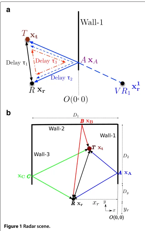
For ease of exposition we start with a single reflecting surface such as the side wall of a building as shown in Figure 1a, considered in two dimensions, with origin “O” shown. The target denoted as (T), radar (R), the vir-tual radar created due to the multipath w.r.t wall-1 and denoted as (VR1) are also shown in the figure. The wall
a
b
Figure 1Radar scene.
assumed for now. The radar and target are located at xr=[−xr,yr]Tandxt=[−xt,yt]T. There are three paths,
shown in Figure 1a, which result in time delays as follows:
τ1=2||xt−xr||/c, τ2=2||x1r−xt||/c,
τ3=τ1/2+τ2/2 (1)
x1r :=[xr,yr]T
where c denotes the speed of light in freespace and is assumed constant throughout. The time delays,τ2andτ3
with τ1 ≤ τ3 ≤ τ2, are referred to as the II-order and
I-order multipath, respectively. The first-order (I-order) multipath incorporates one reflection at wall-1, while the second-order (II-order) multipath incorporates two reflections at wall-1. Rewriting (1), we may express the relationship between the location and time-delay variables as
(xt−xr)2+(yt−yr)2=c2τ12/4 (2a)
(xt+xr)2+(yt−yr)2=c2τ22/4 (2b)
x2t c2τ2
3/4
+ (yt−yr)2
(c2τ2
3−4x2r)/4
=1. (2c)
It is readily seen that (2a) and (2b) are the equations of circles, whereas (2c) is the equation of an ellipse which has its foci at the radar, xr and thevirtual radar at x1r, consistent with a bistatic radar configuration.The circles and ellipses in (2) are the loci or the iso-range contours traced by target and its multipath w.r.t wall-1([14], p.42). It may then be shown that the common intersection point of (2a)–(2c) is the target locationxt. When the measured time delaysτi,i = 1, 2, 3 are substituted in (2), the target may be non-coherently localized, provided the multipath and direct path are detectable and resolvable in the range profile [1]. The multipath therefore createsvirtual mono-static andvirtualbistatic receivers aiding localization with a single real monostatic sensor. It is assumed through-out that the multipath radar returns are detectable and resolvable in this article. When this assumption is invalid, multipath exploitation becomes challenging, if possible at all. Given that multipath exploitation is still a relatively emerging topic in radar, as a first step, we are interested in determining performance bounds under idealized con-ditions; investigating performance under conditions when some or all the assumptions start to break down is an interesting topic for future work.
Now consider Figure 1b, which shows an urban canyon type geometry with the target inside the urban canyon, of dimensionD1andD2, respectively. Denote the
multi-path time delays generated from wall-2 asτ4andτ5(τ1≤ τ5 ≤ τ4), and wall-3 asτ6 andτ7(τ1 ≤ τ7 ≤ τ6). The
time delaysτ4andτ6are similar to delayτ2but generated
from double reflections from wall-2 and wall-3 respec-tively. Likewise,τ5andτ7are similar to the delayτ3and
consist of a one-way propagation via the direct line of sight path, and a bounce on the return (or vice versa). Due to these similaritiesτp,p=2,. . ., 7 are not explicitly
shown in Figure 1b. These time delays may be expressed as follows:
τ4=2||x2r−xt||/c, τ5=τ1/2+τ4/2,
τ6=2||x3r−xt||/c, τ7=τ1/2+τ6/2 (3)
x1r:=[xr,yr]T, x2r :=[−xr, 2D2+2Dy+yr]T,
x3r:=[−(2D1−xr),yr]T
for virtual radars at positions xjr,j = 1, 2, 3, and the parameterDythestandoff distanceas shown.
2.1 Multipath preservers
feasible sensor positions, with the objective of maximiz-ing the multipath exploited system performance. Further, these functions could also be used a posterioriin plac-ing some confidence on the target location estimates. The formulation in (1) and (3) assumes that multipath returns are always present for each corresponding wall and was an implicit assumption in [1-7,11-13]. This is in general not true. To understand the reason, consider point A in Figure 1a, having coordinatesxA=[ 0,yA]T, yA(xr,xt):=
ytxr+xtyr
xt+xr , and explicitly a function of the radar and target coordinates. Clearly, for multipath to exist for this wall, we must have thatDy+yr yA D2+Dy+yr. We can
now formulate a multipath preserving function, denoted asf1(yA),
f1(yA)=1Dy+yryAD2+Dy+yr, (4)
where1[·] is the indicator function. In essence, (4) implies that if pointAis not on its respective wall, then no multi-path is observed, which impliesτ3= τ2= 0. In the same
spirit, we may derive the multipath preserving functions for the other two walls in Figure 1b as
f2(xB)=1[0xBD1], (5)
are the coordinates of pointsBandCin Figure 1b, respec-tively. The conditions in (4), (5), (6) are derived from simple geometrical constraints; hence, the coordinates of the points, A,B,C are the functions of both xt and xr. When the need arises, their dependence onxrandxtwill explicitly be noted.
Incorporating multiple (more than 2) reflections at mul-tiple walls and their corresponding multipath preservers into our model is straightforward, but is not considered here as the radar returns associated with multiple reflec-tions have low signal power due to two factors (ignoring the radar cross section of the target itself ): the path loss and the reflection coefficients. The path loss is inversely proportional to a function of the distance traveled by the individual multipath. In general, for each signal reflection a fraction of the incident power is lost, and is related to the reflection coefficient for that particular wall. The reflec-tion coefficients in turn depend on the material prop-erty of the walls as well as the incidence and refraction angles. If indeed multipath from such multiple reflec-tions are detectable and resolvable, it may be shown from the results in the next section that localization will only improve in the CRB sense. Although not treated explicitly
here, note that inclusion of a front wall in say Figure 1b yields a through-wall radar scenario [12,15] in which case the analysis here provides a valid approximation, for example whenDyD1,D2.
3 CRBs and BCRBs
We now proceed to derive expressions for lower bounds on the target localization error co-variance in classical and Bayesian settings. To do so, we express the FIM in terms of the assumed to be known (up to additive Gaussian noise) multipath delays, and incorporate the multipath preserver functions from the previous section. The target localiza-tion error covariance matrix is then lower bounded by the CRB, i.e., the inverse of the FIM. In the Bayesian setting where we assume prior statistics on the target location, the target localization error covariance is bounded by the BCRB—the inverse of the analogous Bayesian information matrix (BIM).
If s(t) is the signal transmitted by the radar, then in general, the received radar return denoted by sr(t) is
expressed as
where ρp captures the strength of the various direct
and multipaths, vc(t) is the clutter in sr(t), and vn(t)
is the noise. Although not explicitly stated, we have assumed an omni-directional radar, and in practice the
ρp will also depend on the antenna pattern. In general, it is noted that the direct and multipath each have dif-ferent SNRs as well as different signal-to-clutter ratios (SCRs) as captured by the different ρp,p = 1, 2,. . ., 7.
In essence, their individual SNRs and SCRs will affect their detectability in the range profile, and is not the focus here. In other words, we will assume that the τp
are all detectable in the range profile. Modeling urban clutter is difficult, and moreover not straightforward to model stochastically. We will therefore ignore clutter and treat only the noise in the FIM and BIM analysis. Clutter however is discussed in Section 5, and incor-porated as spurious time delays in the simulations, i.e. Section 6.
In practice, the time delays, τp, p = 1,. . ., 7 are obtained from correlating the transmitted signal with the received radar returns, see for example [1]. It is there-fore reasonable to assume that the measured time delays, denoted asζp, are perturbed versions of their true
coun-terparts. The perturbations denoted asvpare assumed to
be zero mean, normally distributed, and mutually uncor-related random variables of variance σp2. Therefore, the p-th time delay measurement,ζp, is given by
wheref(1) = 1,f(2) = f(3) = f1(yA), f(4) = f(5) =
f2(xB), andf(6)= f(7)= f3(yC). The assumption of
nor-mality imposed on thevpensure analytical tractability of
the CRBs. If the τp are well separated in theτ domain,
which is the case for large bandwidth, then thevpmay be
modeled as uncorrelated; this is our assumption.
3.1 CRBs
The CRB for target localization is given by the inverse of the FIM for target locationxt. We break the complete FIM down into its various components, i.e., first, we examine the FIM considering only the multipath and direct path w.r.t to each wall independently. LetFk(xt)denote the FIM considering only wallk= 1, 2, 3 assumingx1t :=[xt,yt]T,
i.e., suppressing the negative sign ofxt in xt. Using (7) and for the time being assuming that the corresponding multipath preservers are unity,
where ‘’ denotes the Hadamard product or elementwise multiplication,τk:=[τ2k,τ2k+1], and
From here onward and for notational succinctness, we will drop the explicit dependency of matrices Gk on (σ2k,σ2k+1). The partial derivatives in (8) are obtained
from (1) and (3). As an example the partial derivatives to computeF1(xt)are now given
Using (9), the following matrix can readily be constructed:
∂τ1 (10). From (8), we note that if any one of the multipath preservers in (4), (5), or (7) is zero, then those corre-sponding FIMs are rank deficient and hence singular at the corresponding target locations.
The complete FIM incorporating all the multipath time delays and the direct path is given by
F(xt)=
From (11), it is seen that richer resolvable multipath mechanisms improve the CRBs by adding more statisti-cal information to the FIM. The same conclusion can be made if we were to include higher-order multipath from multiple reflections as discussed in Section 3, provided of course they are detectable. From (11), notice that forF(xt) to be full rank and hence nonsingular, at least one matrix must satisfy
Equation (12) implies that apart from the direct path time delay, and regardless of the values assumed by the multi-path preservers, at least one of the multimulti-path time delays
τp,p = 2,. . ., 7 must be detectable in the τ-domain.
Indeed if it is knowna priorithat the target is shadowed (no direct path time delay,τ1), then at least any two of the
multipath time delays must be detectable or identifiable in theτ-domain.
Until now we considered only two dimensions, however, for the complete 3D problem, we may extend our results in a straightforward manner, for example, by taking the right-hand side of (12) to be 2 instead of 1, and withxtnow comprising the downrange, crossrange, and height param-eters, and with suitable modification of the time delays to incorporate the 3D structure.
corresponding multipath preservers are unity. The FIMs
evaluated at only those target locations which yield unit values for their corresponding multipath preservers. For all other locationsFkare rank-1 and hence singular, which
implies that unbiased estimation of the target is not possi-ble. On the other hand, it is clear thatFis non-singular at those target locations where at least one of the multipath preservers are unity.
3.2 BCRBs
Assume that prior surveillance has made available the information that the target is located in a certain region inside the urban canyon in Figure 1b. As an example and an envisaged scenario, a prior unmanned aerial vehi-cle visit to the canyon has detected possible targets in a certain area, and has directed further investigation via a single-sensor, land-based radar. In such situations, BCRBs [16] are useful in analyzing the system performance.
Assume for simplicity that the target is uniformly distributed in (−xmax,ymax) × (−xmin,ymin) inside the
canyon. The joint probability density function ofxtandyt
is then,
Note that we may incorporate different distributions of the target priors; this uniform distribution example is just a simple initial example of how one would go about obtaining the BCRBs. Let us define the measured time delay vector,ζ =[ζ1,. . .,ζ7]T, andp(ζ,xt,yt)as the joint
pdf ofζ,xt, andyt. Then the BIM which considers
multi-path from all the walls is
B=E
a non-informative prior. For other distributions assumed, the second term will be non-zero. The BIM considering
the direct path and the multipath from thek-th wall is then given by
Bk =
xmax,ymax
xt=xmin,yt=ymin
Fk(xt,yt)dxtdyt, k=1, 2, 3. (15)
Like the classical CRBs, the BCRBs are present on the diagonals of the inverted BIMs. Unlike the FIMs, the BIMs are not a function of the target position vector,xt; they are a function of the radar locationxr.
Some of the double integrals for computing the BIMs are intractable and expressed as integrals of elliptic inte-grals [17]. For example, consider the element in the first row, first column of matrix Bk,k = 1, 2, 3. It is readily
shown that the following term is required to obtain the BIMs:
Considering the integral w.r.txt, and decomposing the
whose first and second parameters represent the complex amplitude and complex modulus, respectively [17]. Simi-larly the integralIcmay be evaluated employing the elliptic
integralF(·,·).
The above are an example of computations needed to evaluate one term in the BIM; there exist many such terms which are evaluated as integrals of F(·,·) and E(·,·). Numerical integration is employed in evaluating the BIMs for two reasons. First, the incomplete ellip-tic integrals are themselves evaluated numerically, see for example [17] and references therein. Second, it can be shown that the functions whose integrals we seek have no singularities in the region of interest as long as
suppp(xt,yt)⊆ ℵ, for any valid distributionp(xt,yt),
where ‘supp’ denotes support. Numerical integration may produce erroneous results when regions include the sin-gular points; but no such problems occur here since we consider only meaningful target priors, i.e., those whose supports are entirely inside the urban canyon.
4 Target or sensor positioning using statistical experimental design
The FIMs and BIMs not only provide us with theoreti-cal bounds on lotheoreti-calization error variance when exploit-ing resolvable multipath, but they may also be of use in designing radar experiments which seek to maximize the ability to exploit multipath. That is, radar operators may wish to either determine where targets are best localized, or where sensors must be placed in order to best localize (surveillance). These optimization problems may be posed in terms of statistical experimental design theory using several optimal design criteria [8].
4.1 Optimal positions for target localization given fixed radar position
Consider the situation where we have only a single wall, as in Figure 1a, with corresponding FIMF1(xt). The radar operator wants to knowa prioriwhere the target is best localized via multipath exploitation. Although in practice this is of course not in our control, but rather useful to know since estimated locations in the vicinity or at the optimal positions could be assigned as high confidence targets. Let us consider theD-optimal design, which max-imizes the determinant of the FIM, and therefore min-imizes the generalized variance of the optimal location estimate vector,xˆt [8]. Cast as an optimization problem for fixedxr, we have,
max xt
detF1(xt) (17)
s.t yA(xr,xt)≤D2+Dy+yr,−yA(xr,xt)≤ −(Dy+yr)
Solving (17) via the Karush–Kuhn–Tucker (KKT) con-ditions, one can show there exist multiple optimal solu-tions forxtwhich must satisfy
x2t+(yt−yr)2−x2r =0, A1xt+b1≤0 (18)
A1:= −(D2D+Dy) xr
y −xr
,
b1:= −xrx(D2+Dy+yr) r(Dy+yr)
.
In (18) the first condition is an equation of a circle, whereas the second is the affine inequality constraint which is identical to the multipath preserver in (4) but in matrix form. Using the same approach, i.e. when we opti-mizeFk(xt),k=2, 3 instead, the corresponding circles are given by
ForF2:(xt+xr)2+(yt−D2−Dy−yr)2
−(D2+Dy)2=0
ForF3:(xt+D1)2+(yt−yr)2−(D1−xr)2=0.
(19)
The optimal target locations w.r.t. these walls must sat-isfy their corresponding circles in (19) and corresponding multipath preservers in (5), respectively. These optimal circles comprising the optimal target locations follow a simple pattern:from the radar atxrdraw three lines, one to each wall, or its imaginary extension, which intersects it at a 90 degree angle. Then, the points of intersections with the walls or their extensions are the respective centers of the circles, and the distance of the centers from the radar loca-tion are the respective radii. It is further stressed that these optimal circles in (18) and (19) are not to be confused with the iso-range contours or constant range loci traced by the target, as in (2).
The optimal target location w.r.t the full FIM (i.e., all walls together) is expressed as follows:
max xt
detF(xt) (20)
s.t yA(xr,xt)≤D2+Dy+yr,−yA(xr,xt)≤ −(Dy+yr)
xB(xr,xt)≤D1,−xB(xr,xt)≤0
yC(xr,xt)≤D2+Dy+yr,−yC(xr,xt)≤−(Dy+yr).
4.2 Optimal radar position for Bayesian target localization
Now consider positioning the sensor, when one has some form of a priori knowledge of the target location. This is well suited to a Bayesian approach where we seek to determine the sensor position xr which minimizes the determinant of the BIM (again usingD-optimal criteria). We start again by designing the best sensor position in the presence of one of the three walls at a time, i.e., we express this as three separate optimization problems:
max
The first constraint in (21) states that the radar position cannot be in the target prior pdf support. The second con-straint states that a radar position is considered feasible if alltarget positions within the prior pdf ’s support satisfy their respective multipath preservers. It is not insightful to consider a particular radar position which does not sat-isfy the multipath preserversfor alltarget positions within the support of the target prior pdf. It is noted that for the urban canyon this is NOT restrictive-since meaningful target priors are defined inside the urban canyon. Closed form solutions to (21) are intractable, but are evaluated numerically in Section 6.
The sensor positioning optimization for the general BIM (all walls together) is
max
The first constraint in (22) is identical to that in (21). The second constraint states that a radar position is consid-ered feasible if it belongs to least one of thek,k=1, 2, 3,
as defined in (21). It is noted that there are several other design criteria, however as stated in ([8], p.153),D-optimal designs are practically relevant. A closed form solution to (22) is not possible, and the optimization will be per-formed numerically in Section 6. It is stressed that these computations may be performed offline, i.e., during the sensor deployment phase. In practice and unlike other optimization problems, it is noted here that the number of variables to be optimized is three or two, depending on the 3D or 2D model, hence computational complexity may not be an issue.
5 Other relevant topics pertinent to localization It is stressed that the main focus of this article is to deter-mine the performance bounds on single sensor target localization via multipath exploitation, as well as sen-sor and target positioning using statistical experimental design. In the previous sections, the experimental design techniques and the lower variance bounds on the tar-get location were formulated under somewhat idealized assumptions: that the time-delays were already estimated and associated to each of the resolvable multipath com-ponents, that all reflections were specular, and that there was no clutter present. In this section however, we com-ment briefly on these ideal assumptions and their impact on target localization.
5.1 Multipath association
In (7), we assumed that we had estimates of the time-delays which were correctly associated with each of the multi-path returns (i.e., which wall and which path for that wall). Going back one step, in the measured range pro-file, even if the time delays are resolvable, they are not necessarily ordered as inτi,i = 2,. . ., 7. They are rather
naturally ordered in an ascending order w.r.t their mea-sured distances. The question is now, how to associate each of the time-delays to the different paths.
The first time delay, being the shortest, may be asso-ciated with the direct path. Labeling the remaining time delay peaks in the range profile may be accomplished by noting that the second order multipath, namelyτp, p = 2, 4, 6 and the first-order multipath, namelyτq,q=3, 5, 7
share a linear relationship with the direct path,τ1given by,
τq=τ1/2+τp/2. (23)
Clustering first- and second-order multipath and wall association is briefly discussed next for completeness; more details are in [1]. Using (23) and employing a search using a least squares utility function, the first-order and second-order multipaths may be clustered together. Let us assume that the clusters are denoted as vectors given byτA,τB,τC. After clustering, their wall associations are still unknown. Since there are three clusters to be associ-ated to the three walls, there exist 3! permutations. Let us denote the permutations or models asMj,j=1, 2,. . ., 3!. Let the mean vector under the assumption of correct wall association be denoted asτo. Now consider another model-dependent vector τ˜(Mj) = Pjτ, where τ =
[τ1,τTA,τBT,τTC]T andPj are the associated permutation
matrices, with the special case of P1 being the identity
matrix of appropriate dimensions. With the distribution assumptions in (7), for the correct model, the random vector τ˜(Mj)−τo has zero mean, and for other
covariance matrix after say maximum likelihood estima-tion of the target locaestima-tionxt, then correct wall association
given by the indexˆjis deduced from
ˆ
j= arg min
j∈{1,2,...,3!}
ln det{C(Mj)} (24)
The location estimates atˆjare the estimates of the target locations at the correct wall association. The cost func-tion in (24) is the standard informafunc-tion-theoretic model selection criteria, albeit without the penalizing function [18]. Not surprisingly, the penalty is irrelevant here since the free parameters for the 3! models are identical to one another. This implies that the error residuals (after max-imum likelihood estimation) may be used equivalently instead of (24) for associating the multipath with the walls. Let us denoteτ¯oas the measured or extracted time delays
whose elements are ordered identical to those inτo. Now ifτj(xˆjt)is the estimated time delay vector as a function of thejth location estimatexˆjt, then thejth model residual,
Rj, is defined asRj= || ¯τo−τj(xˆjt)||2.
5.2 Clutter
Clutter creates spurious time delay peaks in the radar range profile which are readily confused with genuine tar-gets. However, clutter may be mitigated in certain circum-stances. In urban scenarios where there is rich multipath, the assumption that targets are stationary may not neces-sarily be true, i.e., urban targets are often moving, albeit slowly. Furthermore, urban radar scenes consist of several stationary fixtures (or clutter), for example lamp-posts, billboards, signs, etc. which could highly be reflective. If a pulse-Doppler framework is advocated, then stationary clutter such as those described may be mitigated using simple moving target indication (MTI) techniques such as the delay line canceler [19]. For example, using the simplest two-tap delay line canceler results in the single sensor technique providing location updates repeatedly after two consecutive pulse repetition periods throughout the coherent processing interval (CPI). This is more than sufficient for urban targets since they are slowly moving.
In general, standard MTI may be sufficient to mitigate radar returns from stationary clutter, however, there could be scenarios where MTI is imperfect and clutter returns are persistent. Furthermore, MTI does not mitigate inter-actions between the moving targets and stationary clutter. For such relatively rare (but possible) scenarios, clutter manifests as spurious persistent peaks in the range profile. The multipath clustering search described in the previ-ous section to label and cluster the first- and second-order multipath before wall association proves useful in isolat-ing the clutter time delays, provided they are not confus-able with the multipath returns, i.e., follow for example,
(23) with other multipath time delays. Simulation exam-ples with extraneous clutter time delays, and application of the clustering to identify them is demonstrated in Section 6 for multiple targets.
5.3 Impact of wall roughness
Thus far, we have considered smooth surfaces which result in ideal specular reflections for the multipath. We investi-gate if this is realistic, and whether wall roughness would impact localization via multipath exploitation. In partic-ular, when the wavelength is comparable to the rough-ness/depth of groves (craters) in the walls, we ask whether this leads to severe scattering with several diffuse mul-tipath components and smearing, and if so, how would it affect the time-delay estimates, when compared to the ideal case of smooth scattering from walls. To perfectly address the impact of wall roughness, a full investiga-tion using electromagnetic (EM) theory would be needed; which necessitates, in part, knowledge of the material properties of the walls, and the various angles of inci-dence to compute the equivalent reflection coefficients but for the diffuse multipath components. Here, we take a higher-level signal processing approach and use sim-ple, analytically tractable models to evaluate these effects, to obtain an approximate sense of the impact of wall roughness on localization.
EM conditions which describe wall roughness into classes, smooth, slightly rough, moderately rough, and very rough can be seen in [20], which furthermore provides a good introduction to modeling rough sur-faces via radar. Interestingly, from [20], it maybe con-cluded that for a given incidence angle, a surface appears rough with decreasing wavelengths, and independent of wavelength, a surface appears smooth as the incident angle increases. Typically in urban scenarios, to facili-tate operational covertness large standoff distances maybe employed, which lead to large incident angles for most walls. EM intensive bistatic and backscattering models for rough walls are beyond the scope of analysis here, but could be seen in [21-24] and references therein.
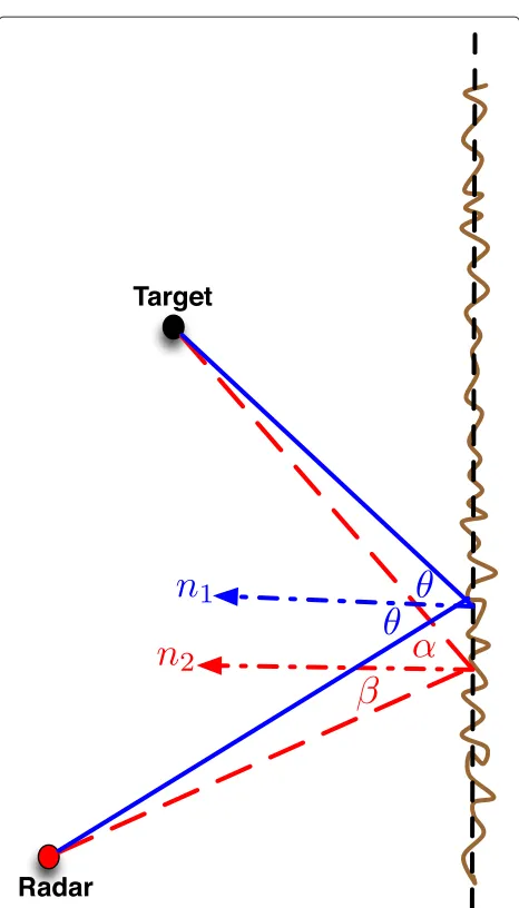
Consider Figure 2 which shows an exaggerated rough-ness texture of say wall-1. The solid blue line is the spec-ular second-order multipath, and the red dashed-dotted line is one of the many diffuse second-order multipaths. The baseline smooth wall is also shown in this figure. The specular component has the angle of incidence w.r.t to normaln1equal to the angle of reflection,θ. Likewise in
Figure 2, the diffuse component has the angle of incidence,
α which is different and not equal to the angle of reflec-tionβ. It is noted that the normals are w.r.t the baseline smooth walls.
Figure 2Exaggerated wall craters to demonstrate roughness: Dashed black (baseline smooth wall), solid blue (specular multipath), dashed red (diffuse multipath), dashed-dotted red and blue (the normals at the reflection points w.r.t the baseline smooth wall).
therein. That is, to emulate roughness/craters on the wall, we considerNsubreflectors which form the length of the wall(s). Each subreflector is placed at a random depth from the baseline smooth wall. The random depths are chosen from a Gaussian distribution with the means cor-responding to the locations of the baseline smooth walls, and the standard deviation as a percentage of the oper-ating wavelength [5]. To simulate pattern roughness or in other words texture, the random subreflectors may be spatially correlated [5,25]. If the spatial correlation is high, then the craters have a pattern to their roughness; if not, then the roughness is un-patterned. The multipath returns from the N subreflectors are superposed, with
each subreflector contributing diffuse multipath (the red dotted lines in Figure 2).
Since the scattering properties of the random reflec-tors are unknown, we will weight their contribution in the radar returns. Selecting or modeling this weighting function would be an excellent topic for an in-depth EM investigation. Here however, we propose a simple but flex-ible weighting model based on several physical realities in the system. First, it may be shown (using constrained opti-mization and Lagrange multipliers, for example) that the length of the blue specular reflection multipath compo-nent is smaller than any of the diffuse second-order (or higher-order) red multipath components. This leads us to design a weighting function as follows: if a subreflector is closer to the specular point, the overall path length trav-eled is shorter (and hence experiences lower path loss) and its diffuse multipath component is weighted higher when compared to the diffuse multipath from a subreflector which is much farther away from the specular reflection point on the wall. It is however stressed that no specu-lar multipath is intentionally incorporated into our model. This leads to “locally specular” return signal with many diffuse components around the specular reflection but of smaller magnitude.
The model will be evaluated via numerical simulations, and the specific values assumed by the weighting and spatial correlation are seen there. We note that both the weighting and spatial correlation functions are selected from a fairly general class of functions where one parame-ter is tunable—this allows our model to incorporate a wide variety of surfaces.
The diffuse multipath returns from rough walls may per-turb the range-profile and hence the time-delay estimates, which in turn will perturb the target location estimates. We outline the relationship between the two next. Let us consider a single wall at first. Assume that xt := [xt,yt]T is the resultant location perturbation arising
from perturbations in the time delays,τi.
Consider the direct path, first- and second-order multi-path from wall-1, then
τ1+τ1=2||xt−xr+xt||
c ,
τ2+τ2=
2||x1
r−xt−xt||
c ,
τ3+τ3=τ1/2+τ2/2+τ1/2+τ2/2. (25)
Subtracting (1) from (25), we obtain
τ1=
2 c
||xt−xr+xt|| ||xt−xr|| −
1
× ||xt−xr||
τ2=2
c
||x1r−xt−xt|| ||x1
r−xt|| − 1
× ||x1r−xt||
Equation (26) maybe simplified further, in particularτ1
andτ2maybe rewritten as
τ1= the square root. Using this and simplifying the resulting expressions with a binomial expansion results in a linear equation given by
The analysis until now was for a single wall, i.e., wall-1. Incorporating the corresponding matrices and time delay perturbations for the other two walls, we may write
τ =Axt (28)
where the vector τ consists of the direct and multi-path time delay perturbations form the rough walls-1,2,3. The matrixAis similar to matrixA1but in addition con-sists of gradient vectors of the multipath time delays from the other two walls, and is straightforward to compute. The linear system in (28) is overdetermined withxt =
(ATA)−1ATτ as the least squares solution. Equation (28) describes a deterministic relationship between the time delay and location perturbations. Since the wall roughness is modeled stochastically, the perturbation bias and perturbation variance of the location estimates can be analyzed via Monte Carlo simulations using (28), and are shown in Section 6.
We remark that when we incorporate wall roughness, location estimates are biased. It remains to be seen if target location estimates obtained from range profiles generated by EM models would also yield a bias. Never-theless for biased estimates as such, the CRBs previously derived would not be immediately applicable, and biased CRBs could be derived instead [16]. However, if one were to obtain the target location biasesa priori, then we would be able to offset their effect and use the derived CRBs directly. Formally incorporating wall roughness—via this stochastic model—into the previous CRBs and experi-mental design is not straightforward given that the wall
roughness model is random itself. When the wall rough-ness specifications are unknown, such as the location and the depth of each subreflector, which is true in practice, then, it may be more prudent to assume smooth walls and hence directly apply the results derived here.
6 Simulations
We now proceed to examine various aspects of single-sensor localization through multipath exploitation using numerical simulations. All coordinates and dimensions are in meters unless specified otherwise. The standoff dis-tance,Dy= 3, is assumed constant in all the simulations.
The noise varianceσp2=σ2,P=1, 2...7.
6.1 FIMs, multipath preservers, and target positioning
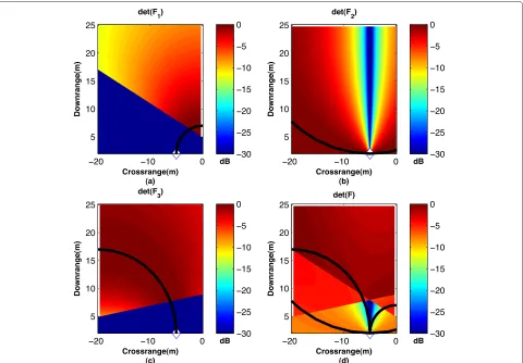
Figure 3 shows the determinant of the FIMs when the radar is assumed to be at positionxr =[−5, 2]T, shown as ♦. The target position is varied in downrange and crossrange inside the urban canyon whose dimensions are D1 = D2 = 20. In these figures, the determinant of
the FIMs are first normalized (the value of σ2 becomes irrelevant) by their maximum value and depicted in the dB scale. The dB scale is employed to clearly show the dynamic range of the experimental design criteria. Here-after, the normalization as well as conversion to dBs will be employed for depicting the design criteria, unless men-tioned otherwise.
In Figure 3a, we consider the direct path and the mul-tipath from the first wall (w1) only, and det(F1)is shown
for varying downrange and crossrange target positions. The blue regions do not experience multipath (multipath blind), as predicted by its corresponding multipath pre-server in (4). The multipath blind zones and visible regions w.r.t Figure 3a are shown in Figure 4a as a binary image. The determinants of the FIMs w.r.t the wall 2,3 are shown in Figure 3b,c, and the corresponding multipath blind and visible zones in Figure 4b,c. The corresponding walls are shown as solid white and red lines in Figure 3 and Figure 4, respectively. It is interesting to note that, for this geome-try, multipath from the second, i.e., the back wall (w2) is always present, as the target’s crossrange is varied within the canyon.
Figure 3Target positioning: walls (in white), for: (a) w1,(b) w2, (c) w3, (d) all, Radar (♦).Part of the optimal circles for walls-1,2,3 as in (18) and (19) are shown with solid black lines.
This is the shadow region, i.e., a region where, if a target was present, nothing behind it would be seen by the radar. Interestingly, the design criteria similar to (17) but for wall-2 chooses this as a multipath blind zone even though the multipath preserver formulation for wall-2 does not take into account whether a point of reflection is in the shadow region; the experimental design however does.
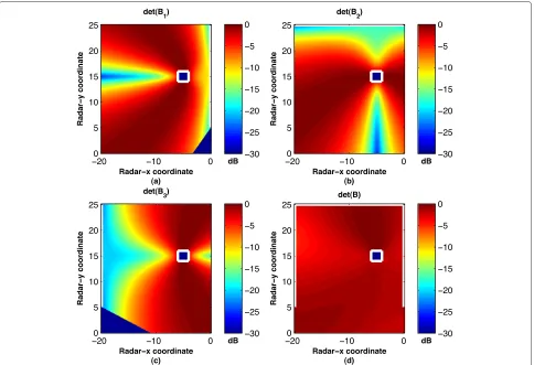
6.2 BIMs and sensor positioning
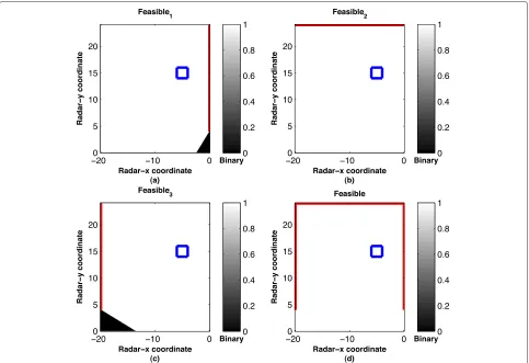
The application of sensor positioning via experimental design is demonstrated next. In Figure 5a–c, the determi-nant of the BIMs are shown when walls 1, 2, and 3 are considered independently, and in Figure 5d when they are considered together. As in the previous case, the multipath blind and visible zones can be inferred from Figure 6a–d, and are determined as explained in the paragraph follow-ing (21). In these figures, the target prior pdf is uniformly distributed over the square with (xmax,xmin) = (6, 4)
and(ymax,ymin) = (16, 14), as shown by. The shadow
region notches are now clearly seen in Figure 5a–c. If the sensor is placed at these notches, then those corre-sponding multipath delays will not exist and cannot be
used for subsequent exploitation. As mentioned before, these shadow region notches are placed automatically by the experimental design criteria and not by the multipath preservers. We see from Figure 5d that some of the opti-mal sensor positions are inside the canyon, and close to the target prior region. It is noteworthy that these optimal sensor positions are not on the boresight(s) of the target prior region. For covertness, it is clear from Figure 5d that the optimal sensor positions outside the canyon and away from the target prior will be preferred.
Figure 4Feasible regions: black (blind), white (visible), walls (red)-(a) w1, (b) w2, (c) w3, (d) all, Radar (♦).
6.3 Multipath association, with and without clutter and higher-order multipath
We now provide a geometric interpretation of the multi-path association algorithm for associating two targets in clutter and higher-order multipath. As detection is not the focus here, a simple peak picking strategy identical to the one used in [1] is used to extract the multipath time delays from the range profile. Three higher-order multi-paths were considered for each of the two targets. The first higher-order multipath consists of the propagation from the radar to the target via one reflection each at walls-1,2, and returning by the same path. The second higher-order multipath consists of the one-way path propagation iden-tical to the first higher-order multipath, but returning to the radar via one reflection at wall-2. Similarly, the third higher-order multipath consists of the one-way path sim-ilar to the first case, and the return path is via a single reflection at wall-3. The first higher-order multipath con-sists of four reflections in total, whereas the second and third consist of three reflections each.
To demonstrate the first- and second-order time delay clustering and wall association, a simulation example is
Figure 5Sensor positioning (BIM): walls (in white), For: (a) w1, (b) w2, (c) w3, (d) all, Target prior ().
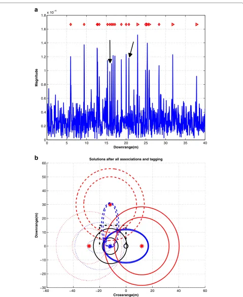
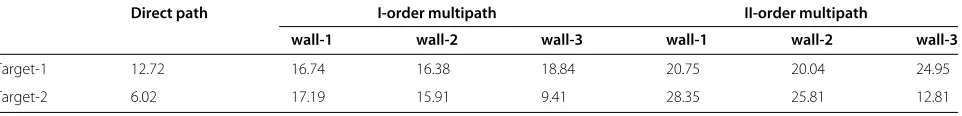
w.r.t the range. The true range of the direct and multipath peaks is given in Table 1. We outline first the clustering, and then the wall association algorithms and demonstrate their performance in simulations.
6.3.1 Clustering of the first- and second-order multipath From Table 1, and from Figure 9a, the first two peaks are at (6.02,9.41) in meters. The algorithm starts by assum-ing that the first peak is the direct path of some arbitrary target. The second peak is initially hypothesized as a first-order multipath, while the remaining peaks are candidate second-order multipaths. The relation between the direct path, I- and II-order multipath as in (23) is then used to identify the correct cluster. Applying this to the spe-cific example, from the candidate II-order multipath time delay estimates, the peak at 12.81 m is selected. Hence (9.41, 12.81) are grouped. Using the same algorithm, the other peaks (15.91, 25.81) and (17.19, 28.35) are grouped for the direct path at 6.02 m. The second target’s direct path, I, and II-order multipath are now clearly identi-fied. Using the same principle, the first target’s direct, I-, and II-order multipath are identified, whereas the clut-ter peaks at 15.33 and 22 m are outliers and are rejected
from the analysis. Similarly, the higher-order multipath are treated as outliers by the clustering algorithm and are rejected. After clustering or grouping the multipath, their wall associations are unknown and are dealt with next.
6.3.2 Wall association
There are six permutations for associating the grouped I- and II-order multipath pairs to the three walls. The permutation with the least cost (cost defined as in (24)), or equivalently corresponding to the least model fitting residual is then selected as the correct wall association.
Figure 6Feasible regions: black (blind), white (visible), walls (red)—(a) w1, (b) w2, (c) w3, (d) all, Target prior ().
residual. This thus allows us to visualize the wall associa-tion algorithm.
The ellipses and circles for the first and second target at the correct wall association is shown in Figure 9b. In this figure, the estimated target locations are shown as (blue square symbol). We have three ellipses correspond-ing to the I-order multipath from walls-1,2,3. Likewise for each target we have four circles, the circle centered at the radar (blue asterisk symbol) is the iso-range contours cor-responding to the direct path. The other remaining circles are centered at the virtual radars (red asterisk symbol), and correspond to the iso-range contours of the II-order multipath from walls-1,2,3. Therefore, in total in Figure 9b we have 6-ellipses and 8-circles.
We examine the intersections of the elliptical and cir-cular loci in Figure 10. In this figure, the circles and ellipses are shown for the six permutations. The grouped multipath corresponding to the first target located at
(−5.6, 11) was used. In Figure 10a, wall-1 association is correct whereas the rest are incorrect. In other words, the ellipses and circles corresponding to wall-1 correctly intersect at the right target location. Similarly, we see from Figure 10c,d that wall-2 and wall-3 associations
are correct, whereas the rest are not. In Figure 10f, all the ellipses and circles intersect the right target loca-tion; this is the correct wall association. It appears that Figure 10d,f is more or less identical. This is not true. The magnified version of Figure 10d in the inset shows three iso-range contours intersecting at one location, whereas the rest of the iso-contours intersect at different loca-tions. In Figure 11a–f, similar elliptical and circular loci are shown but for the second target at (−16, 4.6). The circles and ellipses in Figure 11f correspond to the cor-rect wall association. Interestingly, due to ill-fitting some of the iso-range contours have purely complex parame-ters and are therefore not correctly rendered. For example, and are therefore not correctly rendered. For example, the ellipse corresponding to wall-2 association in Figure 11a,e has a complex minor-axis parameter, and is therefore not correctly shown.
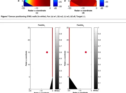
Figure 7Sensor positioning (FIM): walls (in white), For: (a) w1, (b) w2, (c) w3, (d) all, Target (◦).
0 5 10 15 20 25 30 35 40 0
0.2 0.4 0.6 0.8 1 1.2 1.4 1.6 1.8x 10
−4
Downrange(m)
b
a
Magnitude
−60 −40 −20 0 20 40 60
−30 −20 −10 0 10 20 30 40 50 60
Solutions after all associations and tagging
Crossrange(m)
Downrange(m)
Table 1 True range values of direct path (black), I-order multipath (blue) and II-order multipath (magenta) for first target at(−5.6, 11)and second target at(−16, 4.5)
Direct path I-order multipath II-order multipath
wall-1 wall-2 wall-3 wall-1 wall-2 wall-3
Target-1 12.72 16.74 16.38 18.84 20.75 20.04 24.95
Target-2 6.02 17.19 15.91 9.41 28.35 25.81 12.81
estimates. A combinatorial approach as in [1] could used but at a computational cost which increases exponen-tially with the number of targets or clutter time delay peaks. Nevertheless, due to the overdetermined system of equations, correct localization may be achievable by omit-ting the incorrect cluster from the analysis, provided it is identified easily from the circular and elliptical iso-range contour intersections.
6.4 Impact of wall roughness
Finally, we look at the impact of wall roughness on local-ization performance. Range profiles for rough walls after matched filtering are shown in Figure 12, for 1, 3, and 10% roughness in walls-1,2,3. The effects as seen in Figure 12 are for one random realization of the wall roughness per-centages and for one instance of N = 500 equi-spaced randomly generated subreflectors for each wall. The loca-tions of each subreflector on a particular wall is given by a 2D coordinate vector consisting of a determinis-tic x or y coordinate (depends on the wall), and the other coordinate (yorxresp.) whose location (depth) is randomly chosen. The carrier frequency was chosen to be 10 GHz in these simulations. The standard deviation of the random depths of the craters for each subreflec-tor was chosen to be the roughness percentage w.r.t the operating wavelength. The statistical means of the ran-dom depths of the craters were assumed to be identi-cal to the baseline smooth values, as if, the walls were smooth.
The spatial correlation of the random depths of the sub-reflectors are assumed to follow an exponential model with parameter η for walls-1,2,3. Similarly the weight-ing of the multipath returns from each subreflector are also assumed to follow an exponential model but with parameterγ. We denoteZkas thespeculardeterministic x-coordinate (fork= 2) or the speculardeterministicy -coordinate (fork=1, 3) w.r.t wall-k, and similarly denote
Pkn as the corresponding deterministic x-coordinate (k = 2) or the corresponding deterministicy-coordinate (k = 1, 3) of thenth subreflector,n = 0, 1,. . .,N −1. With similar notation let us denoteQknas therandom x -coordinate(k = 1, 3)orrandom y-coordinate(k= 2). It is noted thatZk andPknare deterministic, whereasQkn is random. The weighting function denoted asW(n,k)for the diffuse multipath radar return from thenth subreflec-tor on the kth wall, and the spatial correlation function
denoted asS(n1,n2), between then1th and n2th
subre-flector on the same wall, are given by
W(n,k)=exp(−γ|Zk−Pkn|)
where N(·,·) denotes the standard normal distribution,
λois the operating wavelength, andκ =wall roughness %.
The first- and second-order multipaths from each of these subreflectors are now weighted and superposed along with the direct path, and expressed as
srough(t)=s(t−τ1)
whereτ¯knis the second-order (double bounce) multipath
time delay from thekth wall andnth subreflector,τ1is the direct path. The first-order multipath (single bounce) as before is sum of half the direct, and half the second-order multipath time delay. As a particular example, fork = 1,
¯ generating Figure 12. The canyon dimensions are simi-lar to those used in Figure 3, with the target located at
a
b
c
d
e
f
a
b
c
d
e
f
20 30 40 0
0.05 0.1 0.15 0.2 0.25 0.3 0.35 0.4 0.45
Range (m)
(a)
20 30 40 0
0.05 0.1 0.15 0.2 0.25 0.3 0.35 0.4 0.45
Range (m)
(b)
20 30 40 0
0.05 0.1 0.15 0.2 0.25 0.3 0.35 0.4 0.45
Range (m)
(c)
Figure 12One realization of range profiles after matched filtering for (a) 1%, (b) 3%, and (c) 10% wall roughness.
case. The coherent loss of SNR is also seen in the first- and second-order multipath time delay peaks as they widely fluctuate in their magnitudes for different wall roughness percentages. In certain cases, we see that some of the peaks merge while some them split. All of these effects are due to the random constructive and random destructive phase effects due to the superposition of the diffuse multi-path, and result in perturbation of the time delays leading to perturbation in locations of the target.
6.4.1 Impact of varying wall roughness and diffuse returns weighting.
To evaluate the mean perturbation and the variance of the target perturbation location error, 500 Monte Carlo trials were performed for varying wall roughness and varyingγ.
The target location perturbation is derived from (28) for each trial. The mean and variance of the perturbation are given in Table 2. The locations of the local maximums in the range profile, within a 0.5-m search window on either side of the true locations of the time delays were used in the Monte Carlo analysis. In general from the table, and as expected, the localization perturbation bias increases, whereas the localization perturbation variance decreases for increasing wall roughness percentages. Likewise, both the perturbation bias and variance decrease with increasing weighting, i.e.,γ. Surely, we see some examples especially for the 3 and 10% scenarios, when these trends are not followed. Not much attention needs to be focused on them, as they are attributed to the random effects and warrant more Monte Carlo trials which nevertheless are
Table 2 Perturbation statistics (downrange, crossrange) for fixed spatial correlationη=0.3 and various wall roughness percentages and weighting parameter
Wall roughness (%) 1% 3% 10%
Forγ=0.1
Perturbation bias (m) (0.0246, 0.06) (−0.0039, 0.0882) (−0.0529, 0.1338) Perturbation variance (m2) (0.0001, 0.0001) (0.0022, 0.0011) (0.0121, 0.0024)
Forγ=0.3
Perturbation bias (m) (0.0201, 0.0756) (0.0037,0.0886) (−0.0173, 0.1148) Perturbation variance (m2) (0.0001, 0.0001) (0.0008, 0.0008) (0.0041, 0.0012)
Forγ=0.6
Table 3 Perturbation statistics (downrange, crossrange) for 10% wall roughness percentage, for a fixed weight parameterγ =0.3, and varying spatial correlation,η
Spatial correlation (η) 0.1 0.5 0.99
Perturbation bias (m) (−0.0207, 0.1097) (−0.0212, 0.1189) (−0.0210, 0.1237) Perturbation variance (m2) (0.0023, 0.0012) (0.0041, 0.0014) (0.0044, 0.0014)
computationally heavy. On a global scale such as thel2
-norm of the perturbation bias and variance, these trends are rather followed perfectly.
6.4.2 Impact of varying spatial correlation
The results for the 500 Monte Carlo trials for fixed rough-ness percentages, fixed weighting but for varying spatial correlation are shown in Table 3. An insignificant varia-tion in the results are seen for varying values ofη, implying that texture does not play a large role in target location perturbations. This is to be expected as the depth of sub-reflectors are on the order of wavelengths, which are in millimeters. Hence, their random correlated or random uncorrelated depths will not perturb the diffuse multipath time delays (range) significantly, therefore in general not affecting the perturbation statistics.
6.4.3 Impact of number of sub-reflectors
The results from the 500 Monte Carlo trials with varying number of subreflectors is shown in Table 4. The weight-ing, spatial correlation, and wall roughness are assumed fixed. As a trade-off between computations and accuracy, any value ofNcomparable to the operating wavelength as well as the wall dimensions maybe used for the wall rough-ness model. In our case, the wavelength corresponding to 10 GHz is 0.03 m. The maximum dimensions of the walls are 20 m in thex−ydimensions. Hence, the dimension of each subreflector is 0.2 m forN = 100 and 0.01 m for N = 2000, both of which are comparable to the wave-length. Other values ofN, for exampleN = 10, are not realistic in modeling rough walls for the considered wave-length. From this table whenN = 500, thex-coordinate of the perturbation bias is higher, and may warrant more trials. However, the perturbation bias in they-coordinate is more or less insensitive to changes inN. The perturba-tion variance shows insignificant variaperturba-tion w.r.t changes in Nsince the minimum value ofNassumed already consid-ers several diffuse resolvable and possibly several diffuse unresolvable multipath.
7 Conclusions and future directions
We have performed initial studies into the potential per-formance of the emerging area of single-sensor-based tar-get localization scheme which exploits multipath returns, assuming they are resolvable and the geometry of the reflecting scene is known. To do so, we assumed a single target in a rectangular urban canyon comprised of three walls. For this geometry, Bayesian as well as the classical Cram´er-Rao lower bounds on the target localization error variance were obtained. It was shown that each contribut-ing multipath source, namely the walls, increases the FIM therefore improving the CRBs. Geometrical constraints, termed “multipath preservers” were derived to ensure that multipath was physically observable in the radar returns. Incorporating these into the D-optimal experi-mental design criteria, we demonstrated that FIMs and the BIMs aid in anticipating multipath blind zones, per-mitting optimal sensor or target positioning, and placing confidence levels on the multipath exploitation proce-dures. It was seen via simulations that the experimental design procedures discounted target or sensor positions in the shadow regions.
Wall roughness was incorporated into the radar returns, and its impact was shown on localization. Diffuse mul-tipath from the craters on rough walls led to a bias in the location estimates when compared to the locations estimated from their smooth counterparts. As the wall roughness increases, the location bias increases. Wall association and multipath clustering were shown to be essential for correct localization, and were demonstrated using simulations, and their geometric interpretations, in the presence of extraneous clutter time delay peaks.
In the single-sensor paradigm, there is a scope for future research investigations along several directions. First, one may observe that when multipath is resolvable, it provides the radar operator with additional degrees of freedom. That is, from (7), we see that, in the urban canyon setting with three walls, there are seven multipath components (or equations) and two unknowns, i.e., the elements in
Table 4 Perturbation statistics (downrange, crossrange) for 10% wall roughness percentage,γ =0.5,η=0.3, but for varying number of subreflectors on walls-1,2,3
Number of subreflectors (N) 100 500 1000 2000
![Figure 3 shows the determinant of the FIMs when theradar is assumed to be at position x =[ −5, 2]T, shown](https://thumb-us.123doks.com/thumbv2/123dok_us/905938.1109397/11.595.61.292.118.220/figure-shows-determinant-fims-theradar-assumed-position-shown.webp)