Determination of three-dimensional distribution of electrical conductivity in
the Earth’s mantle from Swarm satellite data: Time-domain approach
Jakub Vel´ımsk´y
Department of Geophysics, Faculty of Mathematics and Physics, Charles University in Prague, Czech Republic
(Received January 11, 2013; Revised June 28, 2013; Accepted August 6, 2013; Online published November 22, 2013)
One of the primary goals of theSwarmmultisatellite mission is to determine the 3-D distribution of electrical conductivity in the Earth’s mantle. This paper presents an inversion method based on direct integration of magnetic fields in the time domain, and using the adjoint solution for fast evaluation of data sensitivities to model perturbations. Two tests of the method are presented. The first one is using a 3-D checkerboard conductivity model and noise-free synthetic data. The second test is based on the closed-loop simulation ofSwarmmission, including recovery of external and induced fields from simulated data along satellite tracks, and realistic noise estimates.
Key words:3-D electromagnetic induction, 3-D inversion, mantle conductivity anomalies, time domain.
1.
Introduction
The method of electromagnetic (EM) induction has long been a standard geophysical tool used to study the elec-trical conductivity of the Earth (Lahiri and Price, 1939; Banks, 1969). On a planetary scale, long-period data (in the period range from few hours to years) from permanent geomagnetic observatories have been traditionally used in 1-D inversions for depth-dependent mantle conductivity structure. Availability of new geomagnetic measurements from low-altitude satellites and from the expanding obser-vatory network has also inspired development of fully three-dimensional (3-D) techniques (Koyamaet al., 2006; Kelbert et al., 2008, 2009; Shimizuet al., 2010; Tarits and Mandea, 2010; Kuvshinov and Semenov, 2012; Semenov and Ku-vshinov, 2012). Thorough reviews of recent advancements in the area of global EM induction are presented by Kuvshi-nov (2008, 2012).
Most of these methods work in the frequency domain, for which the EM induction equation is solved at discrete time-harmonics. The time-domain approaches introduced by Hamano (2002) and Vel´ımsk´y and Martinec (2005) al-low to model EM induction due to transient excitation. This paper presents the development of a 3-D time-domain inver-sion scheme tailored for the upcomingSwarmmultisatellite mission as part of the Swarm Satellite Constellation Appli-cation and Research Facility (Olsenet al., 2013, SCARF). The algorithm uses the time-series of external field Gauss coefficients, and their induced counterparts, obtained by the comprehensive inversion (Sabakaet al., 2013, CI) of Swarm satellite and ground observatory data, and inverts them in terms of 3-D electrical conductivity structure in the Earth’s mantle.
Copyright cThe Society of Geomagnetism and Earth, Planetary and Space Sci-ences (SGEPSS); The Seismological Society of Japan; The Volcanological Society of Japan; The Geodetic Society of Japan; The Japanese Society for Planetary Sci-ences; TERRAPUB.
doi:10.5047/eps.2013.08.001
The key features of the algorithm are described in Sec-tion 2. The results of two basic tests of the method: a noise-free checkerboard test demonstrating the spatial resolution under ideal conditions, and a closed-loop test allowing for direct comparison with the complementary frequency-domain chain (P¨uthe and Kuvshinov, 2013, 3FDI), are pre-sented in Section 3. In the last section, the results, and out-looks for further development of the method are summa-rized.
Electrical resistivityρis used throughout Section 2 to al-low simple notation in theB-field formulation, and to pre-serve compatibility between the manuscript and the actual software implementation. Electrical conductivityσ =1/ρ is preferred in Section 3, discussions, and plots for easy comparison with the accompanying paper (P¨uthe and Ku-vshinov, 2013).
2.
Inverse Modelling in the Time Domain
2.1 Forward problem
A detailed description of the forward solver used in this work is given by Vel´ımsk´y and Martinec (2005). Here we give only a brief overview.
The magnetic field B(r;t) inside a conductive, non-magnetic, solid spherical Earth of radius a with three-dimensional, isotropic distribution of electrical resistivity ρ(r) > 0, and under the magneto-quasistatic approxima-tion (σ ω), is subject to the induction equation,
∇ ×[ρ(r)∇ ×B(r;t)]+μ0
∂B(r;t)
∂t =0. (1) Herer=(r, )=(r, ϑ, ϕ)is the position vector described by radius, colatitude, and longitude in spherical coordi-nates, t is time, and μ0 is the magnetic permeability,
as-sumed to be that of non-magnetic geomaterial in the scope of global EM induction problem. The magnetic field in the insulating atmosphere above the conductive sphere, but be-low the region of magnetospheric electric currents (which
are present at radial distances greater than some radiusb) is described by scalar magnetic potentialU(r;t),
B(r;t)= −∇U(r;t). (2)
The potential satisfies the Laplace equation,
U(r;t)=0, a ≤r≤b, (3)
and therefore can be written in terms of infinite series of real, fully normalized spherical harmonic functions Yj m(),
The setup of the problem doesn’t take into account iono-spheric electric currents flowing above the Earth’s surface, but below the satellite orbit, and their induced counterparts in the Earth (Kuvshinov, 2008, and references therein). These signals must be modelled separately, and subtracted from the magnetic field in the preprocessing, making use of linearity of the induction equation (1). This approach is in-deed applied in the CI processing of satellite data (Sabaka et al., 2013), which employs also the ground observatory data to resolve the ionospheric currents from the induced currents.
The time series of coefficients G(j me)(t), andG(
i)
j m(t) de-scribe the spatio-temporal evolution of the primary mag-netic field of the electric currents in the magnetosphere, and the secondary electric currents induced in the conductive Earth, respectively. They are related to the traditional set of Gauss coeffcientsgj m,hj m,qj m,sj m in Schmidt’s semi-normalization (Langel, 1987) by equations,
G(j mi) =
The series of coefficients, and therefore the summation in Eq. (4) is truncated at a finite degree jmax. Assuming
con-tinutity of magnetic fieldBacross the Earth’s surfacer=a, and expressingBin the base of vector spherical harmonic functions combined with finite elements in the radial direc-tion, the Eqs. (1)–(2) can be discretized and coupled. Given the resistivityρ(r), and the source model G(j me)(t), the for-ward solution is integrated from the initial condition,
B(r;0)=0, (7)
to provide a time series of induced coefficientsG(j mi)(t). The original approach to the integration introduced in Vel´ımsk´y and Martinec (2005) was based on a semi-implicit scheme that treated implicitly the dominant effect of 1-D resistivity profile for stability, while the effects of lateral
variations were taken from the previous time step. How-ever, this approach yields large inaccuracies in the evalua-tion of data sensitivities based on the adjoint problem so-lution, as described in the next section. Therefore, a new version of the program was developed (Kuvshinovet al., 2010), based on an unconditionally stable, second-order accurate Crank-Nicolson integration scheme (Presset al., 1992, chapter 19). Such approach leads to a banded linear system of equations; however, the width of the band can become large since it depends on jmax2 . Factorization of a large, wide-banded linear system, and its repeated solutions at each time step are CPU-intensive. They were therefore paralellized on a distributed-memory architecture, using the ScaLAPACK and MPI libraries (Blackford et al., 1997). The matrix structure invites paralellization by layers, where each computational node stores the matrix and solution for at least 4 adjacent layers. Therefore, for optimal efficiency, the total number of layers in the forward modelling should be divisible by 4.
2.2 Inverse problem
In order to formulate the inverse problem, the resistivity distribution in the Earth is first described by a finite number of model parameters. Spherical harmonic expansion in K discrete layers is used, following similar setup by Kelbertet al.(2008) and P¨uthe and Kuvshinov (2013),
log10ρ(r)=
otherwise. Although this parameterization has no phys-ical justification based on the likely geologphys-ical processes in the mantle, detection of small-scale conductivity hetero-geneities, such as related to the subducted crustal slabs in the mantle, is beyond the expected resolution of the Swarm dataset. Moreover, since the input data to the inverse prob-lem are provided in the form of spherical harmonics, it is natural to choose the same basis also for the conductivity model. The coefficients ρkj m are arranged into the model vectormof dimension M. Not necessarily all coefficients are included inm, andM ≤ K(jmaxρ +1)2. At the start of
the inversion process, selected coefficients can be set to a-priori values, and excluded fromm. This allows for a flex-ible setup of the inverse problem, such as combination of layers with different lateral resolution, and uniform layers.
To solve the inverse problem, one seeks a modelm˜λthat minimizes the penalty function
F(m;λ)=χ2(m)+λR2(m), (9)
whereχ2(m)is the data misfit,λis the regularization
pa-rameter, andR2(m)is the regularization term described in
Subsection 2.3.
The data misfitχ2(m)measures the difference between the observed data, and data predicted by forward modelling for given modelm. We define
χ2(m)=
j m
× external and internal field coefficients, provided in time in-terval (t0,t1)with their respective error estimates δ(j me)(t), δ(i)
j m(t). They are obtained from the satellite data by the process of comprehensive inversion (Sabakaet al., 2013), which involves separation of fields of core, lithospheric, and magnetospheric origin, and their induced counterparts. Since this is basically a least-square fit of spherical har-monic coefficients into data along satellite tracks and on surface, the CI is capable of providing not only coefficient errors, but even full covariance matrices, including covari-ances between external and internal field coefficients.
The summation limits in Eq. (10) are the same as in Eq. (4). If a particular coefficient is not provided by the dataset, we set formally 1/δ(e) coefficients are predicted by the forward solver for each par-ticular modelm. As for the external field which is required as the boundary condition for the forward solver, the obvi-ous choice is settingG(j me)(m;t)=G(j me,obs)(t), independent ofm, which also cancels the first part of integral in Eq. (10). This means that we assume perfect knowledge of the source field, and discard any information about its uncertainty pro-vided by errorsδ(j me)(t). The time interval(t0,t1)can span
the entire duration of the mission or only selected subset. However, the initial timet0at which the evaluation of
mis-fit starts should be chosen at least few days later than the zero time of the initial condition (7) of the forward problem. In this way, the transient (switch-on) effect is minimized (Vel´ımsk´y and Martinec, 2005; Vel´ımsk´yet al., 2006).
Two additional properties of definition (10) are worth mentioning. Firstly, in the (however unlikely) case of error estimates independent of spherical harmonic degree and order,δ(j me)(t)=δ(j mi)(t)=δB(t), Eqs. (2) and (4) lead to
where S = 4πa2 is the surface of the spherical Earth.
Therefore, the data misfit corresponds to a dimensionless, weightedL2norm of differences between the predicted and observed magnetic fields over the Earth’s surface and time. The presence of j,(j+1), and(2j+1)factors in Eq. (10) is thus justified. Secondly, a straightforward generalization of definition (10) that would take into account entire covari-ance matrices is possible. Use of the time-dependent co-variance matrices, or, at least, their diagonal partsδ(j mi)(t)−2,
allows selective downweighting of coefficients poorly con-strained by the CI, i.e., due to temporary data gaps at indi-vidual satellites, or a particulary disadvantageous geometry
of the satellite constellation. However, allowing for uncer-tainties in the external field would require its coefficients to be incorporated in the model vectorm, and then recovered by the inversion jointly with the conductivity model.
Returning back to the problem of minimization of penalty function F(m;λ), several effective multidimensional
al-gorithms, such as conjugate gradients or quasi-Newton method (Presset al., 1992, chapters 10.6–7), are based on the computation of the gradient of the function F(m;λ)in the space of model parameters,
∇mF(m;λ)= ∇mχ2(m)+λ∇mR2(m). (12)
Effective evaluation of the first term is not trivial. The straightforward approach would be to solve 2M +1 for-ward problems for small perturbations of the modelminto each direction in the model space. Then, by numerical dif-ferentiation, we could obtain an approximation of∇mχ2.
Here we use a different approach based on the adjoint method (McGillivrayet al., 1994; Dornet al., 1999; Ficht-ner, 2011). Direct differentiation of (10) yields
∇mχ2=
The adjoint method allows us to evaluate ∇mχ2 without
explicit knowledge of ∇mG(j mi). It reduces the computa-tional burden to the solution of one forward and one adjoint problem. Following a similar derivation as for the 2-D ax-isymmetric case (Martinec and Vel´ımsk´y, 2009), we define the adjoint magnetic field Bˆ(r; ˆt), and magnetic potential
to normal time, starting from the end of the dataset. The adjoint external field is given by the residua of the forward problem,
and the initial condition for the adjoint field is
ˆ
B(r; ˆt =0)=0. (18)
i.e., the adjoint source is compatible with the initial condi-tion (18).
Application of the operator∇mto Eq. (1), multiplication byBˆ, integration over time interval(t0,t1)and volume of
the sphere G, and finally, use of the Gauss theorem and integration per parts, yields after some algebra,
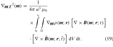
∇mχ2(m)= 1
Differentiating the resistivity with respect to any parameter ρk
Integration of (19) is therefore straightforward with only one caveat. In order to know the adjoint solutionBˆ at timetˆ, Eq. (17) requires that the forward solution is known for all timest ≥t1− ˆt. The forward and adjoint problems cannot
be solved concurrently, the forward problem must be solved first, the entire solutionB(r;t)stored, and then the time in-tegration of Eq. (19) is performed together with the inte-gration of the adjoint problem. The large memory require-ments are handled by parallel distribution to the computa-tional nodes, using the layer structure already established for the forward solver to minimize data transfers between nodes.
2.3 Regularization
The purpose of the regularization term is to control over-fitting of data by unrealistic, spurious oscillations of the resistivity model. Two regularizations were implemented, constraining the first and second derivative, respectively,
R21(m)= 1
Because the forward solver represents resistivity on a grid, the spatial derivatives in the regularizations (21)–(22) are evaluated numerically using a simple 3-point finite-difference stencil (Fornberg, 1996).
The trade-off between the data misfitχ2(m), and the
reg-ularization R2(m)in Eq. (9) is governed by the choice of the regularization parameterλ. The optimal value ofλ is selected by an L-curve analysis (Hansen, 1992). A local minimumm˜λof the penalty function F(λ;m)is found for several values ofλ. Then, the data misfitχ2(m˜λ)is plotted
versus regularizationR2(m˜λ), and the maximum inflection
pointλ˜ of the curve is found visually, using refined sam-pling ofλin its vicinity, as necessary. The corresponding modelm˜λ˜ then represents the solution of the regularized in-verse problem.
2.4 Quasi-Newton minimization
Our implementation of quasi-Newton minimization closely follows the method described in Presset al.(1992, section 10.7). For a givenλ, and starting modelmλ0, the al-gorithm gradually builds an approximation of the inverse Hessian from the values of F(mλi) and ∇mF(mλi) using the Broyden-Fletcher-Goldfarb-Shanno formula. Line min-imization along a given direction uses Brent’s method to proceed to the next iteration point mλi+1. The iteration
terminates when the difference of two successive models
mλi+1−mλi, or the gradient∇mF(mλi)drops below a spec-ified tolerance, or after a maximum number of iterations is reached. Experiments have shown that faster convergence is achieved when the initial modelmλ0is chosen as the optimal resultm˜λ from a run with stronger regularization,λ > λ. Therefore, runs for individual values ofλare chained in de-scending order.
3.
Results
3.1 Checkerboard test
In this section we present the results of two tests of the time-domain 3-D spherical conductivity inversion method. The purpose of the first test is to determine the resolution of the method under idealized conditions with no source of errors. The target 3-D conductivity model, as shown in the right panel of Fig. 1, is based on the 1-D conductivity pro-file of Kuvshinov and Olsen (2006), resampled to 200 km layers spanning the entire crust and mantle. Using the ex-pansion (8), the 1-D model thus defines the coefficientsρk
00.
Over the 1-D background a 3-D checkerboard-like structure is superimposed (Kelbertet al., 2008). The coefficientsρk
32
are set to±1.0 with the sign alternating between layers. The scaling is such that the lateral contrast in each layer is about 0.8 orders of magnitude. All other coefficients describing the model are zero. At the top of the conductivity model, an empirical surface conductance map scaled to a common thickness of 10 km is imposed. It is based on bathymetry, topography, and electrical conductivity of seawater, crys-talline rocks, and sediments, and assembled using the pro-cedure described by Everett et al.(2003). The electrical conductivity of the core is assumed to be 105S·m−1.
The target conductivity model is excited by an external magnetic field represented by spherical harmonic coeffi-cients for orders j = 1,2,3, and degreesm = −1,0,1. The length of time series is 4 years with uniform 1.5 hr sam-pling interval. The induced field coefficients are evaluated by the forward solver up to degree and order 5. Homoge-neous errorδ(j mi)(t)=1 nT is assumed. These settings rep-resent a rather optimistic expectation of the spatio-temporal resolution of magnetospheric field and their induced coun-terparts by the Swarm mission (Sabakaet al., 2013).
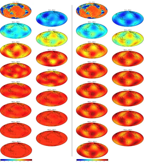
Fig. 1. Checkerboard test: Recovered model (left panel) compared to the target model (right panel). Color cross-sections through individual layers are staggered from top to bottom. Color scale corresponds to log10(σin S·m−1).
structure is well-resolved. In the uppermost mantle, here represented by depth range 10–400 km, the conductive and resistive heterogeneities are well resolved below the resis-tive continents. However, large difference between recov-ered and target model occurs below the oceans, especially the Pacific, a result of strong attenuation of the signal by highly conductive seawater. Below 1000 km, the method is unable to resolve lateral variations of mantle conductivity, and only the 1-D average conductivity is recovered. Con-siderably longer time series would be needed for that task (Vel´ımsk´y and Finlay, 2011).
3.2 Closed-loop test
The second test case uses a target conductivity model that has been designed to test various elements of the SCARF (Olsen et al., 2013), in particular the CI (Sabaka et al., 2013), the 3FDI (P¨uthe and Kuvshinov, 2013), and the 3TDI (this paper).
From top to bottom, the model consists of the surface conductance map scaled to common thickness of 10 km, a 390 km thick resistive layer (0.004 S·m−1) with three
small-scale conductors embedded in it (0.04 S·m−1), a 300 km
heterogene-Fig. 2. Full closed-loop test: Recovered model (left panel) compared to the target model (right panel). Color cross-sections through individual layers are staggered from top to bottom. Color scale corresponds log10(σ in S·m−1), and is identical with the colorscale used in Fig. 3 in the companion 3FDI paper.
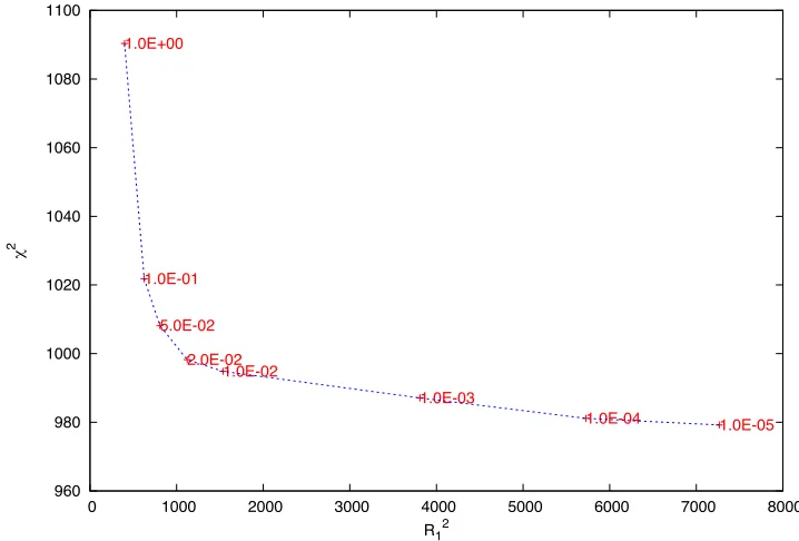
Fig. 3. L-curve used showing the data misfitχ2(m)against the regularization termR12(m)for different values of parameterλ(red numbers) in the closed-loop test.
ity of 1 S·m−1 approximately in the shape of the Pacific
plate, a uniform conductor of 2 S·m−1 down to the
core-mantle boundary, and highly conductive core (105 S·m−1).
The model is shown in the right panel of Fig. 2.
An external field model up to degree 3 and order 1 (in the geomagnetic coordinate system), and with 1 hr sampling interval was derived by analysis of 4.5 years of ground ob-servatory hourly means from July 1998 to December 2002
with 1 hr step, are given in Olsen and Kuvshinov (2004) and Kuvshinov and Olsen (2005).
Realistic Swarm satellite trajectories were simulated for the same period, the external and induced fields were syn-thetized along the tracks with 1 Hz sampling rate, together with other components of geomagnetic field (main, litho-spheric, ionospheric and corresponding induced field), as well as a model of instrument noise. Detailed description on the test dataset assembly is given by Olsenet al.(2006). The CI was then used to reconstruct the individual field components, including the magnetospheric field and its in-duced counterpart (Sabakaet al., 2013).
Thus, the input for the inversion discussed here were 4.5 years long time series of reconstructed external and inter-nal Gauss coefficients in the geomagnetic reference frame. Similarly to the checkerboard test, the external field was truncated at degree 3 and order 1, the internal field was modelled up to degree and order 5. The dipolar coefficients g10,q10 were provided with 1.5 hr sampling, other
coeffi-cients were sampled at 6 hr due to the limited longitudinal coverage of three satellites. Error estimates were also pro-vided in the input dataset.
The coefficients were first preprocessed by rescaling to full normalization, using Eqs. (5)–(6). The non-dipolar co-efficients were interpolated in time by cubic splines to com-mon sampling interval of 1.5 hr. The conductivity model was parameterized using 5 layers each 200 km thick with spherical harmonic expansion truncated at jmaxρ =5. Note
that the layer boundaries used in the inversion do not cor-respond to the layer boundaries of the target model. All computations were performed in the geomagnetic reference frame; however, the final conductivity model was rotated to the geographic coordinate system. The inversion was run using the R1 regularization (21) for 8 values of λ,
rang-ing from 10−5 to 100. Based on an L-curve visual
analy-sis (Fig. 3), we have chosenλ˜ =2×10⁻²as the optimal
balance between data fit and model smoothness.
The resulting model is shown in the left panel of Fig. 2. The recovery of the uppermost 400 km is poor with spu-rious 3-D oscillations present below the oceans, and im-mediately above the large target heterogeneity. These can be assigned to combined effect of surface conductance, as observed in the checkerboard test, with the regularization term constraining the size of the conductivity jump across the 400 km boundary, and the lower sampling rate of non-dipolar coefficients, reducing the information contained in the signal at periods below 1 day, which are the most sen-sitive to upper mantle conductivity. Obviously, given the limited lateral resolution of the data, it is difficult to resolve small scale features present in the upper 400 km. However, the shape and conductivity of the large heterogeneity are well reconstructed in the 400–600 km depth range. In the 600–800 km span, the reconstructed model contains a com-bination of the heterogeneous layer in the target model with the underlying homogeneous, conductive layer; the conduc-tivity below Pacific is well resolved, while the background value is increased elsewhere. Finally, the conductivity of the lower mantle is recovered as a 1-D structure, with small oscillations that are suppressed by regularization.
4.
Conclusions and Outlook
We have developed and tested a new technique to invert a time series of Gauss coefficients representing the exter-nal and interexter-nal magnetic field in terms of a 3-D distribu-tion of electrical conductivity, using direct integradistribu-tion of the magnetic field in the time domain. The approach is designed to process time series provided by the CI for the Swarm multisatellite mission (Olsenet al., 2013), and com-plements a traditional 3FDI approach (P¨uthe and Kuvshi-nov, 2013). We have demonstrated the ability to recover the shape and conductivity of a large heterogeneous sctructure positioned in the mid-mantle from a closed-loop simulation of the Swarm satellite mission that includes realistic model of satellite trajectories, instrument noise, and separation of signals of core, lithospheric, ionospheric, magnetospheric, and induced origin. Moreover, the induced signals for the test dataset were generated using an independent forward solver in the frequency-domain, introducing an additional source of discrepancies in forward modelling. The parame-terization of the model space in the inverse problem did not conform to the target model, both in terms of layer inter-faces positioned at different depths, and sharp lateral con-ductivity contrasts being fitted by spherical harmonics.
The time-domain method, and accompanying programs are currently being expanded. Use of full data covariance matrix, and external field adjustments taking into account its uncertainties are being investigated. Modifications of the regularization methods are also considered. In particu-lar, since the electrical conductivity varies dominantly with depth, separation of the gradient or Laplacian operator in Eqs. (21)–(22) into the radial and angular parts, and down-weighting the first one, could allow for larger radial vari-ability without introducing spurious lateral oscillations to the results of the inverse problem.
Acknowledgments. The software chain described in this pa-per was developed under European Space Agency contract 4000102140/10/NL/1A,Development of the Swarm Level 2 Algo-rithms and Associated Level 2 Processing Facility.The support of the Grant Agency of the Czech Republic, project P210/11/1366, is also acknowledged. I thank M. E. Everett and A. Kuvshinov for their helpful comments.
References
Banks, R. J., Geomagnetic variations and the electrical conductivity of the upper mantle,Geophys. J. R. Astron. Soc.,17, 457–487, 1969. Blackford, L. S., J. Choi, A. Cleary, E. D’Azevedo, J. Demmel, I. Dhillon,
J. Dongarra, S. Hammarling, G. Henry, A. Petitet, K. Stanley, D. Walker, and R. C. Whaley, ScaLAPACK Users’ Guide, Society for Industrial and Applied Mathematics, Philadelphia, 1997.
Dorn, O., H. Bertete-Aquirre, J. G. Berryman, and G. C. Papanicolaou, A nonlinear inversion method for 3D electromagnetic imaging using adjoint fields,Inverse Problems,15, 1523–1558, 1999.
Everett, M. E., S. Constable, and C. G. Constable, Effects of near-surface conductance on global satellite induction responses,Geophys. J. Int., 153, 277–286, 2003.
Fichtner, A.,Full Seismic Waveform Modelling and Inversion, Springer-Verlag, Berlin, Heidelberg, 2011.
Fornberg, B.,A Practical Guide to Pseudospectral Methods, Cambridge Univ. Press, Cambridge, 1996.
Hamano, Y., A new time-domain approach for the electromagnetic induc-tion problem in a three-dimensional heterogeneous earth,Geophys. J. Int.,150, 753–769, 2002.
Kelbert, A., G. D. Egbert, and A. Schultz, Non-linear conjugate gradient inversion for global EM induction: Resolution studies,Geophys. J. Int., 173(2), 365–381, 2008.
Kelbert, A., A. Schultz, and G. D. Egbert, Global electromagnetic induc-tion constraints on transiinduc-tion-zone water content variainduc-tions,Nature,460, 1003–1007, 2009.
Koyama, T., H. Shimizu, H. Utada, M. Ichiki, E. Ohtani, and R. Hae, Water content in the mantle transition zone beneath the North Pacific derived from the electrical conductivity anomaly. inEarth’s Deep Water Cycle, edited by S. Jacobsen and S. van der Lee,AGU Geophys. Monogr. Ser., 168, 171–179, 2006.
Kuvshinov, A., 3-D Global induction in the oceans and solid Earth: Recent progress in modeling magnetic and electric fields from sources of mag-netospheric, ionospheric and oceanic origin,Surv. Geophys.,29, 139– 186, 2008.
Kuvshinov, A., Deep electromagnetic studies from land, sea and space: Progress status in the past 10 years,Surv. Geophys.,33, 169–209, 2012. Kuvshinov, A. and N. Olsen, Modelling the ocean effect of geomag-netic storms at ground and satellite altitude, inEarth Observation with CHAMP, Results from Three Years Orbit, edited by Ch. Reigber, H. L¨uhr, P. Schwintzer, and J. Wickert, 353–358, Springer-Verlag, Berlin Heidelberg, 2005.
Kuvshinov, A. V. and N. Olsen, A global model of mantle conductivity derived from 5 years of CHAMP, Ørsted, and SAC-C magnetic data,
Geophys. Res. Lett.,33, L18301, 2006.
Kuvshinov, A. and A. Semenov, Global 3-D imaging of mantle electrical conductivity based on inversion of observatory C-responses I. An ap-proach and its verification,Geophys. J. Int.,189, 1335–1352, 2012. Kuvshinov, A., J. Vel´ımsk´y, P. Tarits, A. Semenov, O. Pankratov, L.
Tøffner-Clausen, Z. Martinec, N. Olsen, T. Sabaka, and A. Jackson, Level 2 products and performances for mantle studies with Swarm. Swarm Science Study under ESA contract, final report, 2010. Lahiri, B. N. and A.T. Price, Electromagnetic induction in nonuniform
conductors and the determination of the conductivity of the Earth from terrestrial magnetic variations,Phil. Trans. R. Soc. Lond.,A237, 509– 540, 1939.
Langel, R. A., Main field, inGeomagnetism, edited by J. A. Jacobs, 249– 512, Academic Press, London, 1987.
Martinec, Z. and J. Vel´ımsk´y, The adjoint sensitivity method of global electromagnetic induction for CHAMP magnetic data,Geophys. J. Int., 179, 1372–1396, 2009.
McGillivray, P. R., D. W. Oldenburg, R. G. Ellis, and T. M. Habashy, Calculation of sensitivities for the frequency-domain electromagnetic problem,Geophys. J. Int.,116(1), 1–4, 1994.
Olsen, N. and A. Kuvshinov, Modeling the ocean effect of geomagnetic storms,Earth Planets Space,56, 525–530, 2004.
Olsen, N., F. Lowes, and T. Sabaka, Ionospheric and induced field leakage in geomagnetic field models, and derivation of candidate models for DGRF 1995 and DGRF 2000,Earth Planets Space,57, 1191–1196,
2005.
Olsen, N., R. Haagmans, T. J. Sabaka, A. Kuvshinov, S. Maus, M. E. Pu-rucker, M. Rother, V. Lesur, and M. Mandea, The Swarm End-to-End mission simulator study: A demonstration of separating the various con-tributions to Earth’s magnetic field using synthetic data,Earth Planets Space,58(4), 359–370, 2006.
Olsen, N., E. Friis-Christensen, R. Floberghagen, P. Alken, C. D Beggan, A. Chulliat, E. Doornbos, J. T. da Encarnac¸˜ao, B. Hamilton, G. Hulot, J. van den IJssel, A. Kuvshinov, V. Lesur, H. L¨uhr, S. Macmillan, S. Maus, M. Noja, P. E. H. Olsen, J. Park, G. Plank, C. P¨uthe, J. Rauberg, P. Rit-ter, M. Rother, T. J. Sabaka, R. Schachtschneider, O. Sirol, C. Stolle, E. Th´ebault, A. W. P. Thomson, L. Tøffner-Clausen, J. Vel´ımsk´y, P. Vi-gneron, and P. N. Visser, TheSwarmSatellite Constellation Application and Research Facility (SCARF) andSwarmdata products,Earth Plan-ets Space,65, this issue, 1189–1200, 2013.
Pankratov, O., D. Avdeev, and A. Kuvshinov, Electromagnetic field scatter-ing in a heterogeneous Earth: A solution to the forward problem,Phys. Solid Earth,31, 201–209, 1995.
Press, W. H., S. A. Teukolsky, W. T. Vetterling and B. P. Flannery, Numer-ical Recipes in Fortran. The Art of Scientific Computing, Cambridge University Press, Cambridge, 1992.
P¨uthe, C. and A. Kuvshinov, Determination of the 3-D distribution of elec-trical conductivity in Earth’s mantle fromSwarmsatellite data: Fre-quency domain approach based on inversion of induced coefficients,
Earth Planets Space,65, this issue, 1247–1256, 2013.
Sabaka, T. J., L. Tøffner-Clausen, and N. Olsen, Use of the Comprehen-sive Inversion method forSwarmsatellite data analysis,Earth Planets Space,65, this issue, 1201–1222, 2013.
Semenov, A. and A. Kuvshinov, Global 3-D imaging of mantle conductiv-ity based on inversion of observatory C-responses C-responses. II, Data analysis and results,Geophys. J. Int.,191(3), 881–1470, 2012. Shimizu, H., H. Utada, K. Baba, T. Koyama, M. Obayashi, and Y. Fukao,
Three-dimensional imaging of electrical conductivity in the mantle tran-sition zone beneath the North Pacific Ocean by a semi-global induction study,Phys. Earth Planet. Inter.,183, 262–269, 2010.
Tarits, P. and M. Mandea, The heterogeneous electrical conductivity struc-ture of the lower mantle,Phys. Earth Planet. Inter.,183, 115–125, 2010. Vel´ımsk´y, J. and C. C. Finlay, Effect of a metallic core on transient geo-magnetic induction,Geochem. Geophys. Geosyst.,12, Q05011, 2011. Vel´ımsk´y, J. and Z. Martinec, Time-domain, spherical harmonic-finite
ele-ment approach to transient three-dimensional geomagnetic induction in a spherical heterogeneous Earth,Geophys. J. Int.,160, 81–101, 2005. Vel´ımsk´y, J., Z. Martinec, and M. E. Everett, Electrical conductivity in the
Earths mantle inferred from CHAMP satellite measurements, I. Data processing and 1-D inversion,Geophys. J. Int.,166, 529–542, 2006.