Multilevel Mixture Kalman Filter
Dong Guo
Department of Electrical Engineering, Columbia University, New York, NY 10027, USA Email:[email protected]
Xiaodong Wang
Department of Electrical Engineering, Columbia University, New York, NY 10027, USA Email:[email protected]
Rong Chen
Department of Information and Decision Sciences, University of Illinois at Chicago, Chicago, IL 60607-7124, USA Email:[email protected]
Department of Business Statistics & Econometrics, Peking University, Beijing 100871, China
Received 30 April 2003; Revised 18 December 2003
The mixture Kalman filter is a general sequential Monte Carlo technique for conditional linear dynamic systems. It generates sam-ples of some indicator variables recursively based on sequential importance sampling (SIS) and integrates out the linear and Gaus-sian state variables conditioned on these indicators. Due to the marginalization process, the complexity of the mixture Kalman filter is quite high if the dimension of the indicator sampling space is high. In this paper, we address this difficulty by developing a new Monte Carlo sampling scheme, namely, the multilevel mixture Kalman filter. The basic idea is to make use of the multilevel or hierarchical structure of the space from which the indicator variables take values. That is, we draw samples in a multilevel fashion, beginning with sampling from the highest-level sampling space and then draw samples from the associate subspace of the newly drawn samples in a lower-level sampling space, until reaching the desired sampling space. Such a multilevel sampling scheme can be used in conjunction with the delayed estimation method, such as the delayed-sample method, resulting in delayed multilevel mixture Kalman filter. Examples in wireless communication, specifically the coherent and noncoherent 16-QAM over flat-fading channels, are provided to demonstrate the performance of the proposed multilevel mixture Kalman filter.
Keywords and phrases:sequential Monte Carlo, mixture Kalman filter, multilevel mixture Kalman filter, delayed-sample method.
1. INTRODUCTION
Recently there have been significant interests in the use of the sequential Monte Carlo (SMC) methods to solve on-line estimation and prediction problems in dynamic systems. Compared with the traditional filtering methods, the sim-ple, flexible—yet powerful—SMC provides effective means to overcome the computational difficulties in dealing with nonlinear dynamic models. The basic idea of the SMC tech-nique is the recursive use of the sequential importance sam-pling (SIS). There also have been many recent modifications and improvements on the SMC methodology [1,2,3,4,5,6,
7,8,9,10,11,12].
Among these SMC methods, the mixture Kalman filter (MKF) [3] is a powerful tool to deal with conditional dy-namic linear models (CDLMs) and finds important applica-tions in digital wireless communicaapplica-tions [3,13,14]. A sim-ilar method is also discussed in [15] for CDLM system. The CDLM is a direct generalization of the dynamic linear model
(DLM) [16] and it can be generally described as follows:
xt=Fλtxt−1+Gλtut,
yt=Hλtxt+Kλtvt,
(1)
whereut ∼ N(0,I) andvt ∼ N(0,I) are the state and ob-servation noise, respectively, andλt is a sequence of random
indicator variables which may form a Markov chain, but are independent ofut andvt and the pastxsandys,s < t. The matricesFλt,Gλt,Hλt, andKλt are known, givenλt.
An important feature of CDLM is that, given the trajec-tory of the indicator{λt}, the system becomes Gaussian and linear, for which the Kalman filter can be used. Thus, by us-ing the marginalization technique for Monte Carlo computa-tion [17], the MKF focuses on the sampling of the indicator variableλt other than the whole state variable{xt,λt}. This
y
x
c2 c1
c3 c4
s2,2 s2,1
s2,3 s2,4
s1,2 s1,1
s1,3 s1,4
s3,2 s3,1
s3,3 s3,4
s4,2 s4,1
s4,3 s4,4
Figure1: The multilevel structure of the 16-QAM modulation used in digital communications. The set of transmitted symbol A1 =
{si,j, i=1,. . ., 4, j=1,. . ., 4}is the original sampling space, and
the centersA2 = {c1,c2,c3,c4}constitute a higher-level sampling
space.
However, the computational complexity of the MKF can be quite high, especially in the case of high-dimensional in-dicator space, due to the need of marginalizing out the indi-cator variables. Fortunately, often the space from which the indicator variables take values exhibits multilevel or hierar-chical structures, which can be exploited to reduce the com-putational complexity of the MKF. For example, a multilevel structure of the 16-QAM modulation used in digital commu-nications is shown inFigure 1. The set of transmitted sym-bolsA1= {si,j,i=1,. . ., 4, j=1,. . ., 4}is the original
sam-pling space, and the centers A2 = {c1,c2,c3,c4}constitute a higher-level sampling space. Thus, based on the observed data, for every sample stream, we first draw a sample (say c1) from the higher-level sampling spaceA2and then draw a new sample from the associated subspacess1,1,s1,2,s1,3,s1,4of c1in the original sampling spaceA1. In this way, we need not sample from the entire original sampling space, and many Kalman filter update steps associated with the standard MKF can be saved.
This kind of hierarchical structure imposed on the in-dicator space is also employed in the partitioned sampling strategy [18], which greatly improved the efficiency and the accuracy for multiple target tracking over the original SMC methods. However, in this paper, the hierarchical structure is employed to reduce the computational load associated with MKF, especially for high-dimensional indicator space, while retaining the desirable properties of MKF.
Dynamic systems often possess strong memories, that is, future observations can reveal substantial information about the current state. Therefore, it is often beneficial to make use of these future observations in sampling the current state. However, an MKF method usually does not go back to regen-erate past samples in view of the new observations, although the past estimation can be adjusted by using the new impor-tance weights. To overcome this difficulty, a delayed-sample
method is developed [13]. It makes use of future observa-tions in generating samples of the current state. It is seen there that this method is especially effective in improving
the performance of the MKF. However, the computational complexity of the delayed-sample method is very high. For example, for a∆-step delayed-sample method, the algorith-mic complexity isO(|A1|∆), where|A1|is the cardinality of the original sampling space. Here, we also provide a delayed multilevel MKF by exploring the multilevel structure of the indicator space. Instead of exploring the original entire space of future states, we only sample the future states in a higher-level sampling space, thus significantly reducing the dimen-sion of the search space and the computational complexity.
In recent years, the SMC methods have been success-fully employed in several important problems in communi-cations, such as the detection in flat-fading channels [13,19,
20], space-time coding [21,22], OFDM system [23], and so on. To show the good performance of the proposed novel re-ceivers, we apply them into the problem of adaptive detection in flat-fading channels in the presence of Gaussian noise.
The remainder of the paper is organized as follows. Sec-tion 2 briefly reviews the MKF algorithm and its variants. In Section 3, we present the multilevel MKF algorithm. In
Section 4, we treat the delayed multilevel MKF algorithm. InSection 5, we provide simulation examples.Section 6 con-cludes the paper.
2. BACKGROUND OF MIXTURE KALMAN FILTER
2.1. Mixture Kalman filter
Consider again the CDLMs defined by (1). The MKF exploits the conditional Gaussian property conditioned on the indi-cator variable and utilizes a marginalization operation to im-prove the algorithmic efficiency. Instead of dealing with both
xtandλt, the MKF draws Monte Carlo samples only in the
indicator space and uses a mixture of Gaussian distributions to approximate the target distribution. Compared with the generic SMC method, the MKF is substantially more efficient (e.g., it produces more accurate results with the same com-putational resources).
First we define an important concept that is used throughout the paper. A set of random samples and the corresponding weights{(η(i),w(i))}m
i=1 is said to beproperly
weightedwith respect to the distributionπ(·) if, for any mea-surable functionh, we have
m
j=1h
η(j)w(j)
m
j=1w(j)
−→Eπ
h(η) asm−→ ∞. (2)
In particular, if η(j) is sampled from a trial distribution g(·) which has the same support as π, and if w(j) = π(η(j))/g(η(j)), then {(η(j),w(j))}m
j=1 is properly weighted with respect toπ(·).
LetYt = (y0,y1,. . .,yt) andΛt =(λ0,λ1,. . .,λt). By
re-cursively generating a set of properly weighted random sam-ples {(Λ(tj),w(
j)
t )}mj=1to represent p(Λt | Yt), the MKF
ap-proximates the target distribution p(xt | Yt) by a random mixture of Gaussian distributions
m
j=1 w(tj)Nc
µ(j)
t ,Σ
(j)
t
where
are obtained with a Kalman filter on the system (1) for the given indicator trajectoryΛ(tj). Denote
κ(tj) µ
Thus, a key step in the MKF is the production at timetof the weighted samples of indicators {(Λ(tj),κ time (t−1). Suppose that the indicatorλttakes values from
a finite setA1. The MKF algorithm is as follows.
Algorithm1 (MKF). Suppose at time (t−1), a set of property weighted samples{(Λ(t−j)1,κ becomes available, the following steps are implemented to update each weighted sample.
Forj=1,. . .,m, the following steps are applied.
(i) Based on the new datayt, for eachai∈A1, run a one-step Kalman filter update assumingλt=aito obtain
κ(t−j)1 Gaussian and can be computed based on the Kalman filter update (6). Draw a sampleλ(tj)according to the
(iii) Compute the importance weight
wt(j)=w
t } is then properly
weighted with respect top(Λt|Yt).
(iv) Perform a resampling step as discussed below.
2.2. Resampling procedure
The importance sampling weightw(tj)measures the “quality”
of the corresponding imputed indicator sequenceΛ(tj). A
rel-atively small weight implies that the sample is drawn far from the main body of the posterior distribution and has a small contribution in the final estimation. Such a sample is said
to be ineffective. If there are too many ineffective samples, the Monte Carlo procedure becomes inefficient. To avoid the degeneracy, a useful resampling procedure, which was sug-gested in [7,11], may be used. Roughly speaking, resampling is to multiply the streams with the larger importance weights, while eliminating the ones with small importance weights. A simple, but efficient, resampling procedure consists of the following two steps.
t }mj=1 with probability proportional to
the importance weights{wt(j)}mj=1.
Resampling can be done at every fixed-length time inter-val (say, every five steps) or it can be conducted dynamically. The effective sample sizecan be used to monitor the varia-tion of the importance weights of the sample streams and to decide when to resample as the system evolves. The effective sample size is defined as in [13]:
t /m. In dynamic resampling, a resampling
step is performed once the effective sample size ¯mtis below a
certain threshold.
Heuristically, resampling can provide chances for good sample streams to amplify themselves and hence “rejuvenate” the sampler to produce a better result for future states as the system evolves. It can be shown that the samples drawn by the above resampling procedure are also indeed properly weighted with respect to p(Λt |Yt), provided thatmis
suf-ficiently large. In practice, when small to modest mis used (we use m = 50 in this paper), the resampling procedure can be seen as a tradeoffbetween the bias and the variance. That is, the new samples with their weights resulting from the resampling procedure are only approximately proper, and this introduces small bias in the Monte Carlo estimation. On the other hand, however, resampling significantly reduces the Monte Carlo variance for future samples.
2.3. Delayed estimation
Model (1) often exhibites strong memory. As a result, fu-ture observations often contain information about the cur-rent state. Hence a delayed estimate is usually more accurate than the concurrent estimate. In delayed estimation, instead of making inference on Λt instantaneously with the
poste-rior distributionp(Λt|Yt), we delay this inference to a later
As discussed in [13], there are primarily two approaches to delayed estimation, namely, the delayed-weight method and the delayed-sample method.
j=1 contain information about the future observations (yt+1,. . .,yt+δ), the estimate in (11) is
usually more accurate than the concurrent estimate. Note that such a delayed estimation method incurs no additional computational cost (i.e., CPU time), but it requires some ex-tra memory for storing{λ(tj),. . .,λ
(j)
t+δ}mj=1. For most systems, this simple delayed-weight method is quite effective for im-proving the performance over the concurrent method. How-ever, if this method is not sufficient for exploiting the con-straint structures of the indicator variable, we must resort to the delayed-sample method, which is described next.
2.3.2. Delayed-sample method
An alternative method of delayed estimation is to generate both the delayed samples and the weights {(λ(tj),w
(j)
t )}mj=1 based on the observationsYt+∆, hence makingp(Λt |Yt+∆) the target distribution at time (t+∆). The procedure will provide better Monte Carlo samples since it utilizes the fu-ture observations (yt+1,. . .,yt+∆) in generating the current samples of λt. But the algorithm is also more demanding
both analytically and computationally because of the need of marginalizing outλt+1,. . .,λt+∆.
For each possible “future” (relative to timet−1) symbol sequence at time (t+∆−1), that is,
The delayed-sample MKF algorithm recursively propagates the samples properly weighted for p(Λt−1 |Yt+∆−1) to those forp(Λt|Yt+∆) and is summarized as follows.
Algorithm2 (delayed-sample MKF). Suppose, at time (t+∆−
1), a set of properly weighted samples{(Λ(t−j)1,κ steps are implemented to update each weighted sample.
Forj=1, 2,. . .,m, the following steps are performed.
(i) For eachλt+∆=ai∈A1, and for eachλtt+∆−1∈A∆1, per-form a one-step update on the corresponding Kalman filterκ(t+j)∆−1(λtt+∆−1), that is,
Note that the second density in (16) is Gaussian and can be computed based on the results of the Kalman filter updates in (15). Draw a sampleλ(tj)according to
results from the previous step.
(iv) Resample if the effective sample size is below a certain threshold, as discussed inSection 2.2.
Finally, as noted in [13], we can use the above delayed-sample method in conjunction with the delayed-weight method. For example, using the delayed-sample method, we generate delayed samples and weights{(Λ(tj),w
(j)
t )}mj=1based on observationsYt+∆. Then with an additional delayδ, we can use the following delayed-weight method to approximate any inference about the indicatorλt:
Ehλt
|Yt+∆+δ
∼ = 1
Wt+δ m
j=1 hλ(tj)
w(t+j)δ, Wt+δ= m
j=1 wt(+j)δ.
(18)
3. MULTILEVEL MIXTURE KALMAN FILTER
Suppose that the indicator space has a multilevel structure. For example, consider the following scenario of a two-level sampling space. The first level is the original sampling space
ΩwithΩ= {λi, i=1, 2,. . .,N}. We also have a higher-level
sampling spaceΩwithΩ = {ci,i=1, 2,. . .,N}. The
higher-level sampling space can be obtained as follows. Define the elements (say ci) in the higher-level sampling space as the
centers of subsetωiin the original sampling space. That is,
ci=
1
ωi
j
λjI
λj∈ωi
i=1, 2,. . .,N, (19)
whereωi,i = 1, 2,. . .,N, is the subset in the original
sam-pling space
Ω=
N
i
ωi, ωi
ωj= ∅, i,j=1,. . .,N,i=j. (20)
We callcithe parent of the elements in subsetωiandωithe
child set ofci. We can also iterate the above merging
proce-dure on the newly created higher-level sampling space to get an even higher-level sampling space.
For example, we consider the 16-QAM modulation sys-tem often used in digital communications. The values of the symbols are taken from the set
Ω=(a,b) :a,b= ±0.5,±2.5. (21)
As shown inFigure 1, the sampling spaceΩcan be divided into four disjoint subsets:
ω1=
(0.5, 0.5), (0.5, 2.5), (2.5, 0.5), (2.5, 2.5),
ω2=
(−0.5, 0.5), (−0.5, 2.5), (−2.5, 0.5), (−2.5, 2.5),
ω3=
(−0.5,−0.5), (−0.5,−2.5), (−2.5,−0.5), (−2.5,−2.5),
ω4=
(0.5,−0.5), (0.5,−2.5), (2.5,−0.5), (2.5,−2.5). (22)
Moreover, the centers of these four subspaces are c1 = (1.5, 1.5), c2 = (−1.5, 1.5), c3 = (−1.5,−1.5), and c4 = (1.5,−1.5). Thus, we have obtained a higher-level sampling space composed of four elements. Then the MKF can draw samples first from the highest-level sampling space and then from the associated child set in the next lower-level sampling space. The procedure is iterated until reaching the original sampling space.
For simplicity, we will useci,lto represent theith symbol
value in thelth-level sampling space. Assume that there are, in total,Llevels of sampling space and the number of ele-ments at thelth level is|Al|. The original sampling space is defined as the first level. Then the multilevel MKF is summa-rized as follows.
Algorithm3 (multilevel MKF). Suppose, at time (t−1), a set of properly weighted samples{(Λ(t−j)1,κ
(j)
t−1,w (j)
t−1)}mj=1is avail-able with respect to p(Λt−1 | Yt−1). Then at timet, as the new dataytbecomes available, the following steps are imple-mented to update each weighted sample.
Forj=1,. . .,m, perform the following steps.
(A1) Draw the samplec(t,jL)in theLth-level sampling space.
(a) Based on the new data yt, for each ci,L ∈ AL,
perform a one-step update on the corresponding Kalman filterκ(t−j)1(λt−1) assumingct,L=ci,Lto
ob-tain
κ(t−j)1
λt−1 yt,ci,L
−−−→κ(t,ji)
λt−1,ci,L
. (23)
(b) For eachci,L ∈ AL, compute the Lth-level
sam-pling density
ρ(t,iL,j)P
ct,L=ci,L|Λ(t−j)1,Yt
=pyt|ci,L,Λ(t−j)1,Yt−1
Pci,L|Λt(−j)1,Yt−1
. (24)
Note that by the model (1), the first density in (24) is Gaussian and can be computed based on the Kalman filter update (23).
(c) Draw a sample ct(,jL) from the Lth-level sampling
spaceALaccording to the above sampling density,
that is,
Pc(t,jL)=ci,L
∝ρ(t,iL,j), ci,L∈AL. (25)
(A2) Draw the samplec(t,jl)in thelth-level sampling space.
First, find the child setω(lj)in the currentlth-level sam-pling space for the drawn samplec(t,jl)+1in the (l+ 1)th-level sampling space, then proceed with three more steps.
(a) For eachc(i,jl),i=1, 2,. . .,|ω
(j)
l |in the child setω
(j)
l ,
perform a one-step update on the corresponding Kalman filterκ(t−j)1(λt−1) to obtain
κ(t−j)1
λt−1 yt,ci(,jl)
−−−→κ(t,ji)
λt−1,c
(j)
i,l
(b) For eachc(i,jl), compute the sampling density
Note that the first density in (27) is also Gaussian and can be computed based on the Kalman filter update (26).
Repeat the above steps for the next level until we draw a sampleλ(tj)=c
(j)
t,1from the original sampling space. (A3) Append the symbolλ(tj)toΛ
(j)
t−1and obtainΛ (j)
t .
(A4) Compute the trial sampling probability. Assuming the drawn samplec(t,jl)=cti,,ljin thelth-level sampling space and the associated sampling probability isρt(i,l,j), then
the effective sampling probabilityP(λ(tj)|Λ
(j)
t−1,Yt) can be computed as follows:
(A5) Compute the importance weight
wt(j)=w
(A6) Resample if the effective sample size is below a certain threshold, as discussed inSection 2.2.
Remark1 (complexity). Note that the dominant computa-tion required for the above multilevel MKF is the update of the Kalman filter in (23) and (26). Denote J |A1| and Kl |ωl|. The number of one-step Kalman filter updates
in the multilevel MKF is N = L
l=1Kl. Consider the
16-QAM and its corresponding two-level sampling space shown inFigure 1. There areN =8 one-step Kalman filter updates needed by the multilevel MKF, whereas, the original MKF requires J = 16 Kalman updates for each Markov stream. Hence, the computation complexity is reduced by half by the multilevel MKF.
Remark2 (properties of the weighted samples). From (30), we have
Substituting it into (30), and repeating the procedure with wt(−j)2,. . .,w
(j)
1 , respectively, we finally have
w(tj) procedure are properly weighted with respect to p(Λt | Yt)
provided that{Λ(j)
t−1,w (j)
t−1}mj=1are properly weighted with re-spect top(Λt−1|Yt−1).
4. DELAYED MULTILEVEL MIXTURE
KALMAN FILTER
The delayed-sample method is used to generate samples
{(λ(tj),ω
(j)
t )}mj=1based on the observationsYt+∆, hence mak-ing p(Λt |Yt+∆) the target distribution at time (t+∆). The procedure will provide better Monte Carlo samples since it utilizes the future observations (yt+1,. . .,yt+∆) in generating the current samples ofλt. But the algorithm is also more
de-manding both analytically and computationally because of the need of marginalizing outλt+1,. . .,λt+∆.
Instead of exploring the “future” symbol sequences in the original sampling space, our proposed delayed multilevel MKF will marginalize out the future symbols in a higher-level sampling space. That is, for each possible “future” (rel-ative to timet−1) symbol sequence at time (t+∆), that is,
λt,ct+1,l,. . .,ct+∆,l
∈A1×A∆l (l >1), (33)
where ct,l is the symbol in the lth-level sampling space,
we compute the value of a ∆-step Kalman filter {κ(t+j)τ(λt,
recursively propagates the samples properly weighted for p(Λt−1 | Yt+∆−1) to those for p(Λt | Yt+∆) and is summa-rized as follows.
Algorithm4 (delayed multilevel MKF). Suppose, at time (t−
1), a set of properly weighted samples{(Λ(t−j)1,κ as the new data yt+∆becomes available, the following steps are implemented to update each weighted sample.
(A1) For eachλt =ai ∈A1, and for eachctt+1,+∆l ∈A∆l,
per-form the update on the corresponding Kalman filter κ(t+j)∆−1(λt,ctt++1,∆−l1), that is, (A3) Draw a sampleλ(tj) according to the above sampling
density, that is,
(A5) Compute the importance weight
wt(j)=w (A6) Do resampling if the effective sample size is below a
certain threshold, as discussed inSection 2.2.
Remark3 (properties of the weighted samples). Similar to the multilevel sampling algorithm in Section 3, it can be shown that the samples {Λ(j) bution any more, but a mixture of Gaussian components. Since the mixture of Gaussian distribution is implausible to be achieved within the rough sampling space, it has to be ap-proximated with a Gaussian distribution computed by the
Kalman filter assuming that the elements in the higher-level sampling space are transmitted. Therefore, some bias will be introduced into the computation of the weight. On the other hand, we make use of more information in the approxima-tion of better distribuapproxima-tion p(Λ(t−j)1,λ
(j)
t |Yt+∆), which makes the algorithm more efficient than the original MKF.
Remark4 (properly weighted samples). To mitigate the bias problem introduced in the weight computation, instead of (38), we can use the following importance weight:
wt(j)=w
Similar to the multilevel sampling algorithm inSection 3, it is easily seen that the samples {Λ(j)
t ,w
(j)
t }mj=1 drawn by the above procedure are properly weighted with respect top(Λt| Yt) provided that{Λ to get better samples based on the future information, de-layed weight may be very effective. Furthermore, there is no bias anymore in the weight computation although we still ap-proximate the mixture Gaussian distribution with a Gaussian distribution as inRemark 3.
Remark5 (complexity). Note that the dominant computa-tion required for the above delayed multilevel MKF is mainly in the first step. DenoteJ|A1|andM|Al|. The number of one-step Kalman filter updates in the delayed multilevel MKF can be computed as follows:
N=J+JM+· · ·+JM∆=JM∆ +1−1
M−1 . (40)
Note that the delayed-sample MKF requiresJ∆+1Kalman up-dates at each time. Since usuallyMJ, compared with the delayed-sample MKF, the computational complexity of the delayed multilevel MKF is significantly reduced.
Remark6 (alternative sampling method). To further reduce the computational complexity in the first step, we can take the alternative sampling method composed of the following steps.
(3) For eachλt = ai ∈ A1, and for each pathk in the selectedKpaths, perform the update on the corresponding Kalman filterκ(t+j)∆−1(λt,ctt++1,∆−l1,k), that is,
κ(t+j)τ−1
λt,ctt++1,τ−l1,k
yt+τ,ct+τ,lk
−−−−−−→κ(t+j)τ
λt,ctt++1,τ,kl
. (43)
(4) For eachai∈A1, compute the sampling density
ρt(,ji)P
λt=ai|Λ
(j)
t−1
× K
k=1
∆
τ=0
pyt+τ|Yt+τ−1,Λ (j)
t−1,λt=ai,ctt++1,τ,kl
×∆ τ=1
Pckt+τ,l|c t+τ−1,k
t+1,l ,λt=ai,Λ(t−j)1
. (44)
The weight calculation can be computed by (40) for the target distribution p(λt | Yt) or (45) for the target
distri-bution p(λt |Yt+∆). Besides the bias that resulted from the Gaussian approximation inRemark 3, the latter also intro-duces new bias because of the summation overK selected paths, other than the whole sampling space in higher level. However, the first one does not introduce any bias as in
Remark 4. DenoteJ |A1|andM |Al|. The number of one-step Kalman filter updates in the delayed multilevel MKF can be computed asN=JK+M∆.
Remark7 (the choice of the parameters). Note that the per-formance of the delayed multilevel MKF is mainly dominated by the two important parameters: the number of prediction steps∆and the specific level of the sampling spaceAl. With
the same computation, the delayed multilevel MKF can see further “future” steps (larger∆) with a coarser-level sampling space (largerl), whereas it can see the “future” samples in a finer sampling space (smallerl), but with smaller∆steps.
Remark8 (multiple sampling space). InAlgorithm 5, we can also use different sampling spaces for different delay steps. That is, we can gradually increase the sampling space from the lower level to the higher level with an increase in the delay step.
5. SIMULATIONS
We consider the problem of adaptive detection in flat-fading channels in the presence of Gaussian noise. This problem is of fundamental importance in communication theory and an array of methodologies have been developed to tackle this problem. Specifically, the optimal detector for flat-fading channels with known channel statistics is studied in [24,25], which has a prohibitively high complexity. Suboptimal re-ceivers in flat-fading channels employ a two-stage structure, with a channel estimation stage followed by a sequence de-tection stage. Channel estimation is typically implemented by a Kalman filter or a linear predictor, and is facilitated by per-survivor processing (PSP) [26], decision feedback [27], pilot symbols [28], or a combination of the above [29].
Other suboptimal receivers for flat-fading channels include the method based on a combination of a hidden Markov model and a Kalman filtering [30], and the approach based on the expectation-maximization (EM) algorithm [31].
In the communication system, the transmitted data sym-bols{st}take values from a finite alphabet setA1 = {a1, . . .,a|A1|}, and each symbol is transmitted over a Rayleigh
fading channel. As shown in [32,33], the fading process is adequately represented by an ARMA model, whose param-eters are chosen to match the spectral characteristics of the fading process. That is, the fading process is modelled by the output of a lowpass Butterworth filter of orderr driven by white Gaussian noise
αt
=ΘΦ(D)
(D)
ut
, (45)
where Dis the back-shift operatorDk,u
t ut−k;Φ(z)
φrzr+· · ·+φ1z+ 1;Θ(z)θrzr+· · ·+θ1z+θ0; and{ut}is a white complex Gaussian noise sequence with unit variance and independent real and complex components. The coef-ficients{φi}and{θi}, as well as the orderr of the Butter-worth filter, are chosen so that the transfer function of the filter matches the power spectral density of the fading pro-cess, which in turn is determined by the channel Doppler frequency. On the other hand, a simpler method, which uses a two-path model to build ARMA process, can be found in [34]; the results there closely approximate more complex path models. Then such a communication system has the fol-lowing state-space model form:
xt=Fxt−1+gut, (46)
yt=sthHxt+σvt, (47)
where
F
−φ1 −φ2 · · · −φr 0
1 0 · · · 0 0 0 1 · · · 0 0
..
. ... . .. ... ... 0 0 · · · 1 0
, g
1 0 .. . 0
. (48)
The fading coefficient sequence{αt}can then be written as
αt=hHxt, h θ0 θ1 · · · θr
. (49)
In the state-space model,{ut}in (46) and{vt}in (47) are the white complex Gaussian noise sequences with unit variance and independent real and imaginary components:
uti.i.d.∼ Nc(0, 1), vti.i.d.∼ Nc(0, 1). (50)
coefficients{αt}are modeled by the following ARMA(3,3)
process:
αt−2.37409αt−1+ 1.92936αt−2−0.53208αt−3
=10−20.89409u
t+ 2.68227ut−1+ 2.68227ut−2
+ 0.89409ut−3
,
(51)
whereut∼Nc(0, 1). The filter coefficients in (51) are chosen
such that Var{αt} = 1. However, a simpler method, which uses a two-path model to build ARMA process, can be found in [34].
We then apply the proposed multilevel MKF methods to the problem of online estimation of the a posteriori probabil-ity of the symbolstbased on the received signals up to time
t. That is, at timet, we need to estimate
Pst=ai|Yt
, ai∈A1. (52)
Then a hard maximum a posteriori (MAP) decision on sym-bolstis given by
st=arg max ai∈A1
Pst=ai|Yt
. (53)
If we obtain a set of Monte Carlo samples of the transmitted symbols{(S(tj),w
(j)
t )}mj=1, properly weighted with respect to p(St|Yt), then the a posteriori symbol probability in (52) is
approximated by
pst=ai|Yt
∼
= 1
Wt m
j=1
1s(tj)=ai
w(tj), ai∈A1, (54)
withWt
m
j=1w (j)
t .
In this paper, we use the 16-QAM modulation. Note that the 16-QAM modulation has much more phase ambiguities than the BPSK in [13]. We have provided the following two schemes to resolve phase ambiguities.
Scheme1 (pilot-assisted). Pilot symbols are inserted period-ically every fixed length of symbols; the similar scheme was used in [20]. In this paper, 10% and 20% pilot symbols are studied.
Scheme 2 (differential 16-QAM). We view the 16-QAM as a pair of QPSK symbols. Then two differential QPSKs will be used to resolve the phase ambiguity. Given the trans-mitted symbol st−1 and information symbol dt, they can
be represented by the QPSK symbol pair as (rst−1,1,rst−1,2)
and (rdt,1,rdt,2), respectively. Then the differential modula-tion scheme is given by
rst,1=rst−1,1·rdt,1, rst,2=rst−1,2·rdt,2. (55)
The two-QPSK symbol pair (rst,1,rst,2) will be mapped to the 16-QAM symbols and then transmitted through the fading channel. The traditional differential receiver performs the following steps:
rdt,1=rdt,1·r
∗
st−1,1, rdt,2=rst,2·r
∗
st−1,2. (56)
0 5 10 15 20 25
Eb/N0(dB)
10−3
10−2
10−1
100
BER
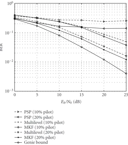
PSP (10% pilot) PSP (20% pilot) Multilevel (10% pilot) MKF (10% pilot) Multilevel (20% pilot) MKF (20% pilot) Genie bound
Figure2: The BER performance of the PSP, MKF, and multilevel MKF for pilot-aided 16-QAM over flat-fading channels.
We next show the performance of the multilevel MKF algorithm for detecting 16-QAM over flat-fading channels. The receiver implements the decoding algorithms discussed inSection 3in combination with the delayed-weight method under Schemes1and2discussed above. In our simulations, we takem= 50 Markov streams. The length of the symbol sequence is 256. We first show the bit error rate (BER) per-formance versus the signal-to-noise (SNR) by the PSP, the multilevel MKF, and the MKF receiver under different pilot schemes without delayed weight inFigure 2and with delayed weight inFigure 3. The numbers of bit errors were collected over 50 independent simulations at low SNR or more at high SNR. In these figures, we also plotted the “genie-aided lower bound.”1 The BER performance of PSP is far from the ge-nie bound at SNR higher than 10 dB. But the performance of the multilevel MKF with 20% pilot symbol is very close to the genie bound. Furthermore, with the delayed-weight method, the performance of the multilevel MKF can be sig-nificantly improved. We next show the BER performance in
Figure 4under the differential coding scheme. As in the pilot-assisted scheme, the BER performance of PSP is far from the genie bound at SNR higher than 15 dB. On the contrary, the
1The genie-aided lower bound is obtained as follows. We assume that
at each timet, a genie provides the receiver with an observation of the modulation-free channel coefficient corrupted by additive white Gaussian noise with the same variance, that is,yt =αt+nt, wherent ∼Nc(0,σ2).
The receiver employs a Kalman filter to track the fading process based on the information provided by the genie, that is, it computesαt=E{αt|yt}.
0 5 10 15 20 25 Eb/N0(dB)
10−3
10−2
10−1
100
BER
PSP (10% pilot) PSP (20% pilot)
Multilevel with delayed weight (10% pilot) MKF with delayed weight (10% pilot) Multilevel with delayed weight (20% pilot) MKF with delayed weight (20% pilot) Genie bound
Figure3: The BER performance of the PSP, the MKF with delayed weight (δ=10), and the multilevel MKF with delayed weight (δ= 10) for pilot-aided 16-QAM over flat-fading channels.
performance of the multilevel MKF is very close to that of the original MKF although there is a 5 dB gap between the genie bound and the performance of the multilevel MKF.
The BER performance of the MKF and the multilevel MKF with or without delayed weight versus the number of Markov streams is shown in Figure 5under the differential coding scheme. The BER is gradually improved from the value 0.16 to the value about 0.08 for multilevel MKF, 0.07 for MKF, 0.065 for multilevel MKF with delayed weight, and 0.062 for MKF with delayed weight with 25 Markov streams. However, the BER performance can not be improved any-more with any-more than 25 streams. Therefore, the optimal number of Markov streams will be 25 in this example.
Next, we illustrate the performance of the delayed multi-level MKF. The receiver implements the decoding algorithms discussed inSection 4. We show the BER performance ver-sus SNR in Figure 6, computed by the delayed-sample or the delayed multilevel MKF with one delayed step (∆=1). The BER performance of the MKF and the MKF with layed weight is also plotted in the same figure. In the de-layed multilevel MKF, we implement two schemes for choos-ing the samplchoos-ing space for the “future” symbols. In the first scheme, we choose the second-level (l =2) sampling space
A2= {c1,c2,c3,c4}, whereci,i=1,. . ., 4, are the solid circles
shown inFigure 1; and in the second scheme, we choose the third-level (l=3) sampling spaceA3 = {c1+c2,c3+c4}. It is seen that the BER of the multilevel MKF is very close to that of the delayed-sample algorithm. It is also seen that the performance of the multilevel MKF method is conditioned on the specific level sampling space. The performance of the
0 5 10 15 20 25
Eb/N0(dB)
10−3
10−2
10−1
100
BER
PSP Multilevel MKF
Multilevel with delayed weight (δ=10) MKF with delayed weight (δ=10) Genie bound
Figure4: The BER performance of the PSP, the MKF, and the mul-tilevel MKF for differential 16-QAM over flat-fading channels. The delayed-weight method is used withδ=10.
0 5 10 15 20 25 30 35 40 45 50
Number of Markov streams 10−2
10−1
BER
Multilevel MKF
Multilevel with delayed weight (δ=10) MKF with delayed weight (δ=10)
Figure 5: The BER performance of the MKF, and the multilevel MKF for differential 16-QAM over flat-fading channels versus the number of Markov streams. The delayed-weight method is used withδ=10.
0 5 10 15 20 25 Eb/N0(dB)
10−3
10−2
10−1
100
BER
MKF
Delayed multilevel sampling (∆=1,l=3) MKF with delayed weight (δ=10) Delayed multilevel sampling (∆=1,l=2) Delayed sample (∆=1)
Genie bound
Figure6: The BER performance of the delayed multilevel MKF with the second (l=2)-level or the third (l=3)-level sampling space for the differential 16-QAM system over flat-fading channels. The BER performance of the delayed-sample method is also shown.
6. CONCLUSION
In this paper, we have developed a new sequential Monte Carlo (SMC) sampling method—the multilevel mixture Kalman filter (MKF)—under the framework of MKF for conditional dynamic linear systems. This new scheme gener-ates random streams using sequential importance sampling (SIS), based on the multilevel or hierarchical structure of the indicator random variables. This technique can also be used in conjunction with the delayed estimation methods, result-ing in a delayed multilevel MKF. Moreover, the performance of both the multilevel MKF and the delayed multilevel MKF can be further enhanced when employed in conjunction with the delayed-weight method.
We have also applied the multilevel MKF algorithm and the delayed multilevel MKF algorithm to solve the problem of adaptive detection in flat-fading communication channels. It is seen that compared with the receiver algorithm based on the original MKF, the proposed multilevel MKF techniques offer very good performance. It is also seen that the receivers based on the delayed multilevel MKF can achieve similar per-formance as that based on the delayed-sample MKF, but with a much lower computational complexity.
ACKNOWLEDGMENT
This work was supported in part by the US National Science Foundation (NSF) under Grants DMS-0225692 and CCR-0225826, and by the US Office of Naval Research (ONR) un-der Grant N00014-03-1-0039.
REFERENCES
[1] C. Andrieu, N. de Freitas, and A. Doucet, “Robust full Bayesian learning for radial basis networks,” Neural Compu-tation, vol. 13, no. 10, pp. 2359–2407, 2001.
[2] E. Beadle and P. Djuric, “A fast-weighted Bayesian bootstrap filter for nonlinear model state estimation,” IEEE Trans. on Aerospace and Electronics Systems, vol. 33, no. 1, pp. 338–343, 1997.
[3] R. Chen and J. S. Liu, “Mixture Kalman filters,”Journal of the Royal Statistical Society: Series B, vol. 62, no. 3, pp. 493–508, 2000.
[4] C.-M. Cho and P. Djuric, “Bayesian detection and estimation of cisoids in colored noise,”IEEE Trans. Signal Processing, vol. 43, no. 12, pp. 2943–2952, 1995.
[5] P. M. Djuric and J. Chun, “An MCMC sampling approach to estimation of nonstationary hidden Markov models,” IEEE Trans. Signal Processing, vol. 50, no. 5, pp. 1113–1123, 2002. [6] A. Doucet, N. de Freitas, and N. Gordon, Eds., Sequential
Monte Carlo in Practice, Springer-Verlag, New York, NY, USA, 2001.
[7] A. Doucet, S. J. Godsill, and C. Andrieu, “On sequential Monte Carlo sampling methods for Bayesian filtering,” Statis-tics and Computing, vol. 10, no. 3, pp. 197–208, 2000. [8] W. Fong, S. J. Godsill, A. Doucet, and M. West, “Monte Carlo
smoothing with application to audio signal enhancement,”
IEEE Trans. Signal Processing, vol. 50, no. 2, pp. 438–449, 2002. [9] Y. Huang and P. Djuri´c, “Multiuser detection of synchronous code-division multiple-access signals by perfect sampling,”
IEEE Trans. Signal Processing, vol. 50, no. 7, pp. 1724–1734, 2002.
[10] A. Kong, J. S. Liu, and W. H. Wong, “Sequential imputations and Bayesian missing data problems,”Journal of the American Statistical Association, vol. 89, no. 425, pp. 278–288, 1994. [11] J. S. Liu and R. Chen, “Sequential Monte Carlo methods for
dynamic systems,”Journal of the American Statistical Associa-tion, vol. 93, no. 443, pp. 1032–1044, 1998.
[12] M. K. Pitt and N. Shephard, “Filtering via simulation: auxil-iary particle filters,”Journal of the American Statistical Associ-ation, vol. 94, no. 446, pp. 590–599, 1999.
[13] R. Chen, X. Wang, and J. S. Liu, “Adaptive joint detection and decoding in flat-fading channels via mixture Kalman fil-tering,”IEEE Transactions on Information Theory, vol. 46, no. 6, pp. 2079–2094, 2000.
[14] X. Wang, R. Chen, and D. Guo, “Delayed-pilot sampling for mixture Kalman filter with application in fading channels,”
IEEE Trans. Signal Processing, vol. 50, no. 2, pp. 241–254, 2002. [15] A. Doucet, N. J. Gordon, and V. Kroshnamurthy, “Particle fil-ters for state estimation of jump Markov linear systems,”IEEE Trans. Signal Processing, vol. 49, no. 3, pp. 613–624, 2001. [16] M. West and J. Harrison, Bayesian Forecasting and Dynamic
Models, Springer-Verlag, New York, NY, USA, 1989.
[17] R. Y. Rubinstein, Simulation and the Monte Carlo Method, John Wiley & Sons, New York, NY, USA, 1981.
[18] J. MacCormick and A. Blake, “A probabilistic exclusion prin-ciple for tracking multiple objects,” International Journal of Computer Vision, vol. 39, no. 1, pp. 57–71, 2000.
[19] D. Guo, X. Wang, and R. Chen, “Wavelet-based sequential Monte Carlo blind receivers in fading channels with unknown channel statistics,” IEEE Trans. Signal Processing, vol. 52, no. 1, pp. 227–239, 2004.
[21] D. Guo and X. Wang, “Blind detection in MIMO systems via sequential Monte Carlo,” IEEE Journal on Selected Areas in Communications, vol. 21, no. 3, pp. 464–473, 2003.
[22] J. Zhang and P. Djuri´c, “Joint estimation and decoding of space-time trellis codes,”EURASIP Journal on Applied Signal Processing, vol. 2002, no. 3, pp. 305–315, 2002.
[23] Z. Yang and X. Wang, “A sequential Monte Carlo blind re-ceiver for OFDM systems in frequency-selective fading chan-nels,”IEEE Trans. Signal Processing, vol. 50, no. 2, pp. 271–280, 2002.
[24] R. Haeb and H. Meyr, “A systematic approach to carrier re-covery and detection of digitally phase modulated signals of fading channels,”IEEE Trans. Communications, vol. 37, no. 7, pp. 748–754, 1989.
[25] D. Makrakis, P. T. Mathiopoulos, and D. P. Bouras, “Opti-mal decoding of coded PSK and QAM signals in correlated fast fading channels and AWGN: a combined envelope, mul-tiple differential and coherent detection approach,” IEEE Trans. Communications, vol. 42, no. 1, pp. 63–75, 1994. [26] G. M. Vitetta and D. P. Taylor, “Maximum likelihood
decod-ing of uncoded and coded PSK signal sequences transmitted over Rayleigh flat-fading channels,”IEEE Trans. Communica-tions, vol. 43, no. 11, pp. 2750–2758, 1995.
[27] Y. Liu and S. D. Blostein, “Identification of frequency non-selective fading channels using decision feedback and adaptive linear prediction,” IEEE Trans. Communications, vol. 43, no. 2/3/4, pp. 1484–1492, 1995.
[28] H. Kong and E. Shwedyk, “On channel estimation and se-quence detection of interleaved coded signals over frequency nonselective Rayleigh fading channels,”IEEE Trans. Vehicular Technology, vol. 47, no. 2, pp. 558–565, 1998.
[29] G. T. Irvine and P. J. McLane, “Symbol-aided plus decision-directed reception for PSK/TCM modulation on shadowed mobile satellite fading channels,”IEEE Journal on Selected Ar-eas in Communications, vol. 10, no. 8, pp. 1289–1299, 1992. [30] I. B. Collings and J. B. Moore, “An adaptive hidden Markov
model approach to FM and M-ary DPSK demodulation in noisy fading channels,” Signal Processing, vol. 47, no. 1, pp. 71–84, 1995.
[31] C. N. Georghiades and J. C. Han, “Sequence estimation in the presence of random parameters via the EM algorithm,”IEEE Trans. Communications, vol. 45, no. 3, pp. 300–308, 1997. [32] G. L. St¨uber, Principles of Mobile Communication, Kluwer
Academic Publishers, Boston, Mass, USA, 2000.
[33] R. A. Ziegler and J. M. Cioffi, “Estimation of time-varying digital radio channels,”IEEE Trans. Vehicular Technology, vol. 41, no. 2, pp. 134–151, 1992.
[34] A. Duel-Hallen, “Decorrelating decision-feedback multiuser detector for synchronous code-division multiple-access chan-nel,”IEEE Trans. Communications, vol. 41, no. 2, pp. 285–290, 1993.
Dong Guo received the B.S. degree in geophysics and computer science from China University of Mining and Technology (CUMT), Xuzhou, China, in 1993; the M.S. degree in geophysics from the Graduate School, Research Institute of Petroleum Ex-ploration and Development (RIPED), Bei-jing, China, in 1996. In 1999, he received the Ph.D. degree in applied mathematics from Beijing University, Beijing, China. He is now
pursuing a second Ph.D. degree in the Department of Electrical En-gineering, Columbia University, New York. His research interests are in the area of statistical signal processing and communications.
Xiaodong Wang received the B.S. degree in electrical engineering and applied math-ematics from Shanghai Jiao Tong Univer-sity, Shanghai, China, in 1992; the M.S. de-gree in electrical and computer engineer-ing from Purdue University in 1995; and the Ph.D. degree in electrical engineering from Princeton University in 1998. From 1998 to 2001, he was an Assistant Professor in the Department of Electrical Engineering,
Texas A&M University. In 2002, he joined the Department of Elec-trical Engineering, Columbia University, as an Assistant Professor. Dr. Wang’s research interests fall in the general areas of computing, signal processing, and communications. He has worked in the areas of wireless communications, statistical signal processing, parallel and distributed computing, and bioinformatics. He has published extensively in these areas. Among his publications is a recent book entitledWireless Communication Systems: Advanced Techniques for Signal Reception. Dr. Wang has received the 1999 NSF CAREER Award and the 2001 IEEE Communications Society and Informa-tion Theory Society Joint Paper Award. He currently serves as an Associate Editor for the IEEE Transactions on Signal Processing, the IEEE Transactions on Communications, the IEEE Transactions on Wireless Communications, and IEEE Transactions on Informa-tion Theory.
Rong Chenis a Professor at the Department of Information and Decision Sciences, Col-lege of Business Administration, University of Illinois at Chicago (UIC). Before join-ing UIC in 1999, he was with the Depart-ment of Statistics, Texas A&M University. Dr. Chen received his B.S. degree in math-ematics from Peking University, China, in 1985; his M.S. and Ph.D. degrees in statistics from Carnegie Mellon University in 1987